ENERGY STAR Building Benchmarking Scores: Good Idea, Bad Science
←
→
Page content transcription
If your browser does not render page correctly, please read the page content below
ENERGY STAR Building Benchmarking Scores: Good Idea, Bad Science
John H. Scofield, Oberlin College
ABSTRACT
The EPA introduced its ENERGY STAR building rating system 15 years ago. In the
intervening years it has not defended its methodology in the peer-reviewed literature nor has it
granted access to ENERGY STAR data that would allow outsiders to scrutinize its results or
claims. Until recently ENERGY STAR benchmarking remained a confidential and voluntary
exercise practiced by relatively few.
In the last few years the US Green Building Council has adopted the building ENERGY
STAR score for judging energy efficiency in connection with its popular green-building
certification programs. Moreover, ten US cities have mandated ENERGY STAR benchmarking
for commercial buildings and, in many cases, publicly disclose resulting ENERGY STAR
scores. As a result of this new found attention the validity of ENERGY STAR scores and the
methodology behind them has elevated relevance.
This paper summarizes the author’s 18-month investigation into the science that
underpins ENERGY STAR scores for 10 of the 11 conventional building types. Results are
based on information from EPA documents, communications with EPA staff and DOE building
scientists, and the author’s extensive regression analysis.
For all models investigated ENERGY STAR scores are found to be uncertain by 35
points. The oldest models are shown to be built on unreliable data and newer models (revised or
introduced since 2007) are shown to contain serious flaws that lead to erroneous results. For one
building type the author demonstrates that random numbers produce a building model with
statistical significance exceeding those achieved by five of the EPA building models.
Introduction
Building energy benchmarking aims to determine how well a particular building
performs with regard to energy use as compared with an appropriate peer group of buildings. The
favored metric for this comparison has been the annual energy use intensity (EUI), calculated by
dividing a building’s annual energy use by its total gross square footage (gsf). Annual energy
used on site, called site energy, is readily determined by totaling monthly energy purchases after
first converting fuel quantities to a common energy unit, typically Btu.1
Site energy, however, fails to account for the off-site losses incurred in producing the
energy and delivering it to the building – particularly important for electric energy that, on
average, is generated and distributed with 31% efficiency [APS, 2008]. The EPA defines
source energy to account for both on- and off-site energy consumption associated with a
building. Source energy is calculated by totaling annual energy purchases after multiplying each
by a fuel-dependent, site-to-source energy conversion factor [EPA SourceE].
1
For site energy calculations 1 kWh of electric energy is equivalent to 3,416 Btu, 1 Ccf of natural gas is equivalent
to 100,000 Btu, etc.
©2014 ACEEE Summer Study on Energy Efficiency in Buildings 3-267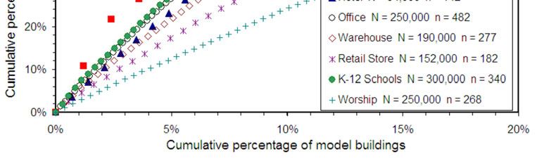
The best source of energy consumption data for commercial buildings traditionally has
   been the Energy Information Administration’s (EIA) Commercial Building Energy Consumption
   Survey that has been conducted every 4-5 years since 1989, with some notable exceptions
   [CBECS]. The last such survey was completed in 2003 and the EIA is now finalizing its 2012
   survey. The 2003 survey contains 5,215 records, each record corresponding to data gathered
   from one sampled building. Collectively these data represent an estimated 4.9 million buildings
   and 72 billion gsf in the U.S. commercial building stock. Hundreds of pieces of information are
   gathered for each sampled building including data for energy use, occupancy, equipment, and
   function.
            The simplest form of benchmarking involves comparing a particular building’s EUI with
   gross EUI for the entire U.S. building stock. 2 Of course a hospital is expected to use more
   energy than an office building, so such broad comparisons have limited value. CBECS identifies
   about 20 different building types in its sampling, allowing one to determine national gross EUI
   for a specific peer group – say just hospitals. CBECS does not identify the location for each of its
   samples but it does identify five climate zones and nine census divisions. To obtain a more
   relevant peer group one can extract CBECS records filtered on such criteria. But with only 5,215
   sampled buildings in CBECS, filtering on more than building type and census division may yield
   only a handful of buildings in the selected peer group – with correspondingly large uncertainties
   in their gross EUI and other statistics.
            In the late 90’s the EPA borrowed methodology then being developed at DOE labs to
   apply regression analysis to CBECS data for benchmarking purposes [Sharp, 1996; Sharp 1998].
   The idea is this. Suppose one intends to benchmark, say, an office building in Topeka, KS. There
   may not be a single sampled office building in CBECS that matches many of the characteristics
   of the one to be benchmarked. But CBECS does include office buildings that are both larger and
   smaller, ones that are older and newer, and so on. Multivariate linear regression analysis is
   applied to all CBECS office buildings to see how their energy use depends on such variables.
   The resulting regression coefficients may then be used to predict the energy use of a hypothetical
   building with characteristics similar to those of the one to be benchmarked. Regression analysis
   has the potential to yield the best of both worlds – the specificity of a narrowly defined CBECS
   query with the statistics of the larger sampled dataset.
            The EPA introduced its ENERGY STAR benchmarking system and score nearly 15 years
   ago. The ENERGY STAR score is an index from 1-100 which is supposed to represent a
   building’s percentile energy efficiency ranking with respect to similar buildings nationally. Over
   the years the EPA has developed ENERGY STAR models (i.e., scoring systems) for 11
   conventional building types, listed in Table 1. The earliest ENERGY STAR building models
   were based on 1995 CBECS data. Models were revised as newer data became available.
            From the outset the EPA’s ENERGY STAR scoring system was a voluntary
   benchmarking tool intended to encourage energy efficiency [Janda and Brodsky, 2000]. Building
   data submitted to Portfolio Manager (the EPA’s web-based tool for calculating scores) and
   ENERGY STAR scores issued by the EPA are confidential – unless a building seeks and
   receives ENERGY STAR certification, in which case its score is 75 or higher and public
   disclosure holds little risk of embarrassment. The EPA has not defended or justified its
   methodologies in any peer-reviewed venues. And, while, for marketing purposes, the EPA

   2
       Gross EUI for a set of buildings is defined to be their total annual energy use divided by their total gsf.

©2014 ACEEE Summer Study on Energy Efficiency in Buildings                                                           3-268
releases selected statistics from data entered into Portfolio Manager it does not otherwise grant
   others access to these data, making it nearly impossible for anyone outside the EPA to scrutinize
   their program, claims, or results.

   Table 1. Table summarizing models for 11 conventional building types where n is the number of
   samples in the regression dataset, N the number of U.S. buildings they represent, R2 the
   goodness of fit for the model regression, and n50 is the number of samples which collectively
   represent 50% of the corresponding national building stock.

            ENERGY STAR            Latest                             regression dataset         # ind. Variables
                                                                                    2
             Building Models      revision      Data Source       n        N      R        n50   explore final
      Residence Hall/Dormitory     Jan-04      CBECS 1999        79     35,000 88%          5     n.a.        4
      Medical Office              Feb-04       CBECS 1999        82     87,000 93%          8     n.a.        5
      Office/Finance/Bank/Court    Oct-07      CBECS 2003       498    250,000 33%         53      27         9
      Retail                       Oct-07      CBECS 2003       182    152,000 71%         30      21        9
      Supermarket/Grocery          Jul-08    CBECS 1999/2003     83      24,000 51%         9      17         7
      Hotel                       Feb-09       CBECS 2003       142      54,000 37%        30      32         6
      K-12 School                 Feb-09       CBECS 2003       353    300,000 27%         70      28        11
      House of Worship            Aug-09       CBECS 2003       269    250,000 37%         59      27         8
      Warehouse                   Aug-09       CBECS 2003       277    190,000 40%         39      26         8
      Senior Care                 Mar-11      Industry survey   553      31,000 43%        85      42        10
      Hospital                    Nov-11      Industry survey   191              22%               26         4

           In the last five years this relatively benign, voluntary benchmarking program has evolved
   into something else. In 2012 the EPA published quantitative claims regarding energy savings
   associated with its ENERGY STAR benchmarking program [EPA DataTrends, 2012]. External
   organizations including the U.S. Green Building Council have adopted the ENERGY STAR
   score as their metric for energy efficiency for green building certification [USGBC]. And a
   growing number of U.S. cities have passed laws requiring owners to benchmark their
   commercial buildings using the EPA’s Portfolio Manager and, in many cases, the resulting
   ENERGY STAR scores are being made public [IMT]. Benchmarking is no longer a voluntary,
   confidential exercise – it is mandatory and real, testable energy claims are being made based
   upon ENERGY STAR scores.
           This expanded use of the EPA’s benchmarking system and, in particular, the public
   disclosure of thousands of building ENERGY STAR scores heightens the need to understand the
   validity of these ENERGY STAR scores and the methodology on which they are based. For
   instance I found ENERGY STAR scores for large office buildings in New York City’s
   publicized 2011 benchmarking data to be unusually high [Scofield, 2013]. David Hsu analyzed
   an expanded, confidential NYC 2011 benchmarking data set and found evidence for significant
   uncertainties in office ENERGY STAR scores [Hsu, 2014]. There is mounting evidence to
   justify a closer look at the methodology and data on which these scores are based.
           Here I summarize the results of an 18-month investigation into the science that underpins
   the EPA’s building ENERGY STAR scores. During this time I have examined, in detail, 10 of
   the EPA’s 11 conventional building models. Information has been gathered from EPA Technical
   Methodology documents, phone and email exchanges with EPA staff as well as building
   scientists at Oak Ridge and Berkeley National Laboratory, and EPA documents obtained through

©2014 ACEEE Summer Study on Energy Efficiency in Buildings                                                          3-269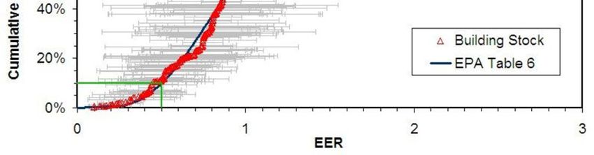
Freedom of Information Act (FOIA) requests. I have also conducted extensive regression
analysis on data that underpin each of the ten building models.
Common Methodology for Producing an ENERGY STAR Score
Below I summarize the key technical steps for developing an ENERGY STAR building
model for a particular type of building [EPA ES-TM]. This description is no-doubt an
oversimplification but provides an adequate description for understanding the rest of this paper.
The first step in the EPA’s model development is to acquire data from a large number of
buildings of a specific building type for use in its linear regression. These data are here referred
to as the regression dataset. The EPA examines these data to identify suitable independent
variables for the regression – ones which demonstrate significant correlation with building
source energy use. Once the regression variables have been identified their regression
coefficients may be used to predict the source energy use for any building of this type for which
data corresponding to the regression independent variables are available. If the benchmarked
building uses less source energy than predicted it is judged to be more energy efficient than its
peer group. The EPA defines a building’s Energy Efficiency Ratio or EER to be the ratio of its
measured source energy to its predicted source energy.3 (Of course source energy is not directly
measured – it is calculated from measured fuel purchases.)
The second step in model development is to generate a distribution of EER’s for the
national stock of buildings of this particular type. This requires a second model dataset, here
called the stock dataset. For most models the regression dataset and stock dataset are identical, or
nearly so.4 The stock dataset contains n samples, indexed j = 1,2,..., n which, with their weights
(wj), represent a total of N w j buildings in the commercial building stock. The model
regression parameters are combined with data from this stock dataset to calculate the EER for
each sampled building. The data are then sorted in order of increasing EER and combined with
the building weights to form a cumulative EER distribution for the national stock of this
particular building type. Such a distribution is graphed in Figure 1 for the EPA’s 2007 Office
building model [EPA Office, 2007].
Steps 1-3 above complete the development of an ENERGY STAR building model. Once
the model is completed the ENERGY STAR score for a particular building is readily determined
from its EER. The ENERGY STAR score is an index (1-100) corresponding to the percentage of
similar buildings in the national building stock that have higher EER’s. Referring to Figure 1, an
office building with an EER = 0.50 receives an ENERGY STAR score of 90 since only 10% of
office buildings nationally have lower EER values.
Note step 2 of the methodology guarantees that the mean score for the represented
building stock will be 50. Moreover, the distribution of scores for the entire building stock will
be uniform – that is, 10% of buildings will have scores from 1-10, another 10% will have scores
from 11-20, and so on.
The above approach generally applies to all 11 of the conventional ENERGY STAR
building models. There are, however, important differences that must be considered on a model
3
This is not quite correct. For early models the EPA performed its regression on the natural logarithm of the source
energy, and the EER = Ln(measured source energy)/(predicted Ln(E)). After 2007 the EPA performed its regression
on the source EUI and defined the EER = (measured EUI)/(predicted EUI).
4
Typically a few outlyers are removed from the stock dataset to form the regression dataset.
©2014 ACEEE Summer Study on Energy Efficiency in Buildings 3-270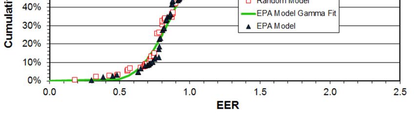
by model basis. In Section 3 below I consider the two oldest building models (Medical Offices
   and Residence Halls/Dormitories). In Section 4 I look at the Office building model whose 2007
   revision represented a significant shift in methodology from that used previously. In Section 5 I
   look at other models developed after 2007 whose methodologies are similar to that employed for
   the 2007 Office model.

           Figure 1. Cumulative EER distribution for the EPA’s 2007 office building model. The blue curve is a 2-
           parameter gamma distribution fit to the data. Horizontal error bars are discussed later in the text.

   Older Models with Regression on Ln(E)
           Early ENERGY STAR building model regressions used the natural logarithm of the
   building source energy, Ln(E), as the dependent variable. This was the case for
   Office/Courthouse/Financial Center/Bank, K-12 schools, Supermarket, Hospitals, Hotels,
   Medical Office, Residence Hall/Dormitory, and Warehouse models, all introduced before 2007.
   As shown in Figure 2, Ln(E) has the advantage of being normally distributed in the building
   stock whereas EUI is not – owing to the fact that EUI cannot be non-negative.5 This has
   implications for regression theory as will be discussed in Section 4.
           Of the models using Ln(E) as the regression variable only those for Medical Offices and
   Residence Hall/Dormitories remain active. Here I discuss the Medical Offices building model.
   All of the features and problems uncovered for this model are also found in the Residence
   Hall/Dormitory model.
           The EPA’s Medical Office model begins by extracting 93 records for medical offices
   from the 1999 CBECS [EPA Medical, 2004]. The EPA claims to reduce this dataset to 82
   records through a series of filters, including the elimination of all buildings less than 5,000 ft2 in
   size. I was not able to replicate this result nor, in response to a FOIA request could the EPA
   supply a list of the buildings in its dataset [FOIA-1, 2013]. Through trial and error, however, I
   was able to identify the 82-building regression dataset on which the EPA’s medical office model

   5
     2003 CBECS data for vacant buildings and records without energy data were removed. Graphs are based on
   remaining 5059 records representing 4.57 million buildings and 69.3 billion gsf.

©2014 ACEEE Summer Study on Energy Efficiency in Buildings                                                          3-271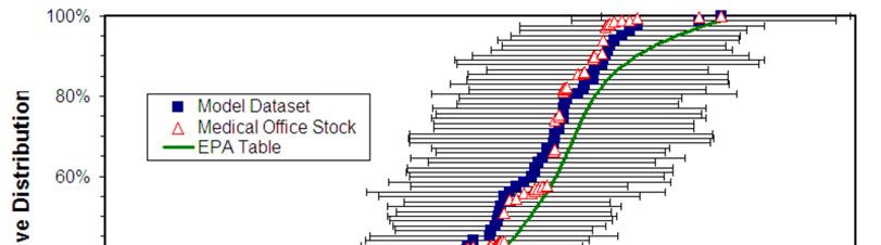
is built. This dataset includes 13 buildings with gsf < 5,000 ft2, corresponding to 50% of the
   87,000 medical offices represented by this dataset [Scofield, 2014].

            Figure 2. Density histogram of the distribution of (a) Ln(E) and (b) EUI for all U.S. commercial buildings
            as captured by the 2003 CBECS. Blue curves represent normal distributions having the same mean and sd
            as the histograms. Ln(E) is close to normally distributed while EUI is not.

           I have used this dataset to replicate the EPA’s un-weighted linear regression on Ln(E)
   (the dependent variable) with five independent variables including Ln(SqFt). My regression
   exactly matches that reported by the EPA with an R2 value of 93% [EPA Medical, 2004].
           The regression coefficients extracted were subsequently used to predict the Ln(E) and
   calculate the EER for each sampled building in the dataset. These data were then combined with
   building weights to produce the cumulative EER distribution for the medical office stock,
   graphed as the open triangles in Figure 3. The EPA, instead, used the EER distribution of just the
   sampled buildings (solid squares) to calculate ENERGY STAR scores, claiming to fit these data
   with a 2-parameter gamma distribution (smooth green curve in Figure 3) [EPA Medical, 2004].6
   I was unable to replicate the fit and the EPA was unable to provide details for such a fit [FOIA-2,
   2013]. Comparing the solid squares with the open triangles it is seen that, for this model, the two
   distributions are not significantly different. For other ENERGY STAR building models
   investigated I have found these differences to be significant.
           In general regression coefficients are no more accurate than the underlying data. The
   EPA publishes standard errors for their regression coefficients but does not further address the
   impact of these errors on ENERGY STAR scores. This issue has been raised in connection with
   Office ENERGY STAR scores contained in New York City benchmarking data [Hsu, 2014].
           I have employed R-software for my regression analysis and utilized the command
   “predict.lm(fit,medical.frame,interval="prediction”, level=0.682)” to produce standard errors for
   predicted Ln(E) values [RProject]. These are then propagated to determine uncertainties in EER,
   shown as the horizontal error bars in Figure 3.7 In the middle of the range these error bars
   6
     The EPA’s describes this process quite differently. The description offered here, however, is mathematically
   equivalent to that used by the EPA.
   7
     Considerable attention has been devoted to the appropriate choice for these error bars. This issue was resolved by
   performing simulations with data for which successive independent variables added to the regression took the R2

©2014 ACEEE Summer Study on Energy Efficiency in Buildings                                                                3-272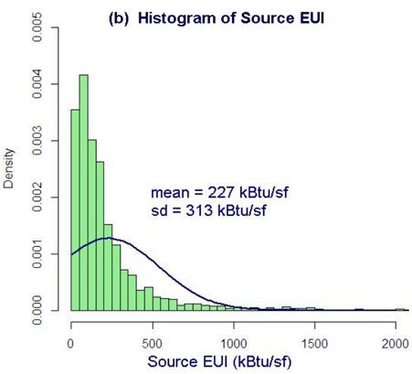
translate into ±35 points uncertainties in the associated ENERGY STAR scores. With such large
   uncertainties there is no statistically meaningful distinction between an ENERGY STAR score of
   75 and one of 50.

            Figure 3. Graph of the medical office cumulative EER distribution for sampled buildings (solid blue
            squares) and the building stock they represent (open red triangles). The solid green curve represents the
            EPA’s fit to the data used for assigning medical office ENERGY STAR scores. The horizontal bars
            represent the standard errors (uncertainties) in EER’s (see text).

           For any regression such as this it is important to consider the reproducibility of the
   underlying data. Would a similar regression performed on a different 82-sample dataset of
   medical offices yield similar results? Ideally this question is addressed by performing the same
   regression on a second independent dataset. This is called external validation. In many cases
   additional, independent data are simply not available. An alternate approach then is to randomly
   divide the original dataset into two subsets, and compare regression results for the two subsets.
   This is called internal validation.
           I have used both internal and external validation tests to determine the validity of this
   model. Data for external validation were obtained from the 2003 CBECS. Both tests found that,
   of the five independent variables, only Ln(SqFt) was a reliable predictor of Ln(E) at the 95%
   confidence level. The other four variables failed both validation tests, suggesting their observed
   correlations with Ln(E) are accidental – unique to this particular 82-building sample rather than
   reflecting a broader trend in the medical office building stock [Scofield, 2014].
           Discussions with staff at the EIA revealed that the EIA did not include statistics for
   Medical Office buildings in their reports because they judged these data to be insufficiently
   robust to produce statistics with less than 10% error. This was confirmed by my own calculations
   of standard relative error (SRE) for the 93 medical office records in the 1999 CBECS data
   [Scofield, 2014].

   from 0 to 100%. Scatter in the data were consistent with error bars produced by the “prediction” option in the
   “predict.lm” R-software command not with those produced using the “confidence” switch.

©2014 ACEEE Summer Study on Energy Efficiency in Buildings                                                              3-273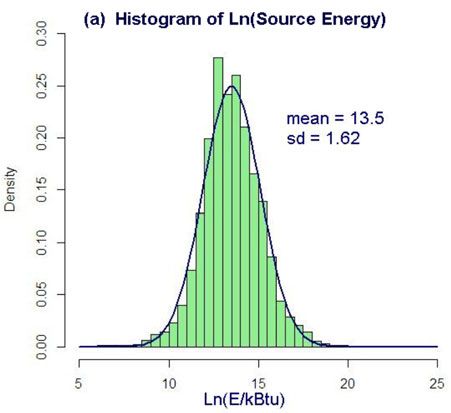
The Office Model
            The most important of the ENERGY STAR building models has always been the Office
   model – which applies to offices, courthouses, financial centers, and banks [EPA Office, 2007].
   The model was introduced in 1999, revised in 2004, and again revised in 2007; the EPA is
   unable to supply documentation for the 1999 version [FOIA-3, 2013]. The 2004 model
   regression was built upon 910 records extracted from the 1999 CBECS data [EPA Office, 2003].
   The EPA identified nine independent variables as key predictors of Ln(E); the regression on
   these produced an R2 of 93%. The 2004 Office model, however, failed to utilize CBECS weights
   for the cumulative EER distribution so that ENERGY STAR scores issued reflected rank among
   sampled buildings not the broader office stock. This failure caused significant error in ENERGY
   STAR scores (discussed below).
            In 2007 the EPA revised its Office model [EPA Office, 2007]. Major revisions included
   1) switching from Ln(E) to source EUI as the regression variable, 2) utilizing data from the
   newer 2003 CBECS, 3) properly utilizing CBECS weights for producing the cumulative EER
   distribution of the office building stock, and 4) using these same CBECS weights for a weighted
   regression. Revision (3) corrected a major flaw in the earlier model, but revisions (1) and (4)
   introduced new errors (discussed below). The revised model performed a weighted linear
   regression on source EUI from 498 CBECS 2003 records using nine independent variables,
   including Ln(worker density) and three variables specific to banks.8 The model regression
   yielded a total R2 value of 33%.9 In this case the EER was defined to be the ratio of the measured
   source EUI to that predicted by the regression.
            The impact of this model revision on ENERGY STAR scores was significant, but would
   have remained hidden except to EPA staff with access to Portfolio Manager data.10 Here I assess
   the impact by comparing scores generated by both models for the same set of office buildings.
   For this purpose I have replicated the EPA’s data filters to extract from CBECS 2003 the Office
   model dataset consisting of 482 records – identical to the EPA’s dataset but lacking the 16
   samples that correspond to courthouses.11 I have used both the EPA’s 2004 Office model and its
   2007 Office model to generate ENERGY STAR scores for these 482 samples and compared the
   results. For several buildings ENERGY STAR scores shifted by 35 points or more. The rms-shift
   in score is 20. While various factors contribute to these shifts in scores it is the correct use of
   CBECS weights in generating the cumulative EER distribution for the 2007 model that had the
   biggest effect.12
            But what of the uncertainties in these scores associated with uncertainties in regression
   coefficients? As for the Medical Office model discussed earlier I have used R-software to

   8
     The EPA defines banks to be buildings classified in CBECS as Bank/Financial with less than 50,000 gsf.
   9
     The EPA’s document explains that the lower R2 value is misleading when compared with that obtained for earlier
   models because the revised model builds in the dominant scaling of Ln(E) with Ln(Sqft) by focusing on EUI (an
   intensive variable) rather Ln(E)
   10
      Individual building managers may have seen large changes in the scores of their buildings, but would have
   remained unaware of the impact on the entire stock.
   11
      Courthouses are not specifically identified in the public version of CBECS 2003, so I am not able to identify these
   records in CBECS. The EIA made these available to the EPA for internal use, but due to security concerns, will not
   make these identities public; their omission has negligible impact on regression results
   12
      This is readily confirmed by modifying the 2004 Office model to properly utilize CBECS weights in producing
   the cumulative EER distribution.

©2014 ACEEE Summer Study on Energy Efficiency in Buildings                                                                  3-274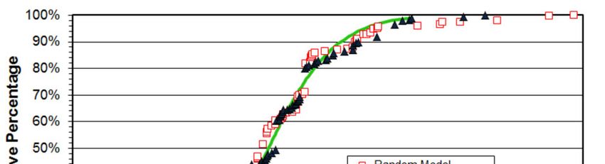
replicate the EPA’s weighted regression, and subsequently used the regression to predict source
EUI for the 482-sample dataset, along with the standard errors in these predicted EUI’s. The
results are combined with building weights to produce the cumulative EER distribution for the
office stock graphed as the open triangles in Figure 1. The curve is indistinguishable from that
published by the EPA [EPA Office, 2007]. I have also calculated the uncertainties in the
predicted EUI with the intention of propagating these to find uncertainties in the corresponding
EER’s. A problem emerges. For about 20% of the buildings in the Office model regression
dataset the uncertainty in the predicted EUI is larger than the predicted EUI – so that the 1-
standard deviation confidence range of EUI includes negative values, This is physically
impossible. This pathological behavior is the result of using source EUI rather than Ln(E) as the
regression variable combined with the low R2 for the regression. EUI data do not satisfy a key
assumption required for regression theory, namely that the deviations of measured EUI from
predicted EUI are normally distributed.
Nevertheless, to gain some understanding of the uncertainties associated with the EPA’s
office ENERGY STAR scores I calculate the uncertainties in EER’s using only the upper bound
for the predicted EUI and, after propagating these errors to EER, use the same error bar on both
sides. These are represented by the horizontal error bars in Figure 1. In the middle of the range
the corresponding uncertainties in ENERGY STAR scores is similar to that seen for the Medical
Office model, 35 points.
I now turn to the error introduced by using CBECS weights in a weighted regression.
Weighted regressions are appropriate when the dependent variables for some samples are known
to higher accuracy than for others. In such cases it is important to force the regression to come
closer to these points since their error bars are smaller [Taylor, 1997]. This is not the case for
CBECS samples. CBECS weights indicate the number of similar buildings that a particular
sample represents in the larger building stock; they are not indicative of the accuracy of data
gathered for a particular sample. Each of the 498 (or 482 w/o courthouses) samples in the office
regression dataset represent an equally valid determination of the dependence of EUI on the
independent variables. Using CBECS weights to weight the regression incorrectly skews the
results. All EPA building models revised or introduced after 2007 suffer from this error.
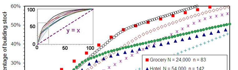
To understand the impact of the weights in a weighted regression consider the
distribution of weights for the Office model dataset, represented by the open black circles in
Figure 4.13 Figure 4 is a graph of the percentage of the total number of buildings N in the
represented stock versus the percentage of the number n of records in the model dataset. If all
records carried equal weight the resulting graph would be a straight line, y = x. Instead the graph
starts out with a steeper slope reflecting the disproportional weight carried relatively few records.
The upper left inset shows the entire range 0-100% while the larger graph expands the scales to
see the weight carried by just 20% of the records in each model dataset.
For the office dataset it is apparent that 7% of the model records represent 33% of the
building stock, hence carry 33% of the regression weight. Weights increase the importance of the
27 bank records in the model dataset by a factor of three. Weighting the regression effectively
reduces the size of the model dataset as the results are determined by relatively fewer buildings.
This has even larger impact on other models where the regression datasets have many fewer than
498 samples. It should be noted that the fewer the samples in the regression dataset the more
susceptible the results are to accidental correlations.
13
Records are sorted in order of increasing weight.
©2014 ACEEE Summer Study on Energy Efficiency in Buildings 3-275
Figure 4. Cumulative weight distributions for the seven post-2007 ENERGY STAR building model
          datasets based on CBECS (see legend). The inset (upper left) shows the full range while the larger graph
          expands the lower end of the scale. Each model dataset contains n samples which collectively represent N
          buildings in the larger building stock.

           I again reproduced the EPA’s 2007 Office model regression, but this time without the
   weighting. The result of this un-weighted regression is that neither Ln(worker density) nor any of
   the three bank variables are significant predictors of EUI. This suggests that these four
   independent variables should be eliminated from the regression.
            In view of the above problems with the 2007 Office model I have decided not to pursue
   further analysis or modification.

   Other Post-2007 Building Models
           The remaining eight building models were developed after 2007. Similar to the 2007
   Office model they (1) employ source EUI rather than Ln(E) as the dependent regression variable
   and (2) incorrectly utilize survey weights to perform a weighted linear regression. Six of the
   models (K-12, Hotel, Warehouse, House of Worship, Supermarket/Grocery Store, Retail Store)
   use CBECS data and CBECS weights. The other two models (Senior Care and Hospital) are built
   upon data gathered through voluntary surveys conducted by the EPA in collaboration with trade
   organizations..
           The distributions of CBECS weights for the relevant models are graphed in Figure 4. I
   now consider the effect of weighted regressions on the other building models.
           Table 1 summarizes features of the model datasets and regressions used for building
   models including revision date, data source, number of buildings (n) in the regression dataset and
   the number (N) they represent in the stock, and the final R2 achieved by the weighted regression.
   Also shown is the number (n50) of samples in the regression dataset which, with their associated
   weights, correspond to 50% of their respective building stocks. These numbers can be
   determined from graphs in Figure 4. For the Supermarket/Grocery Store model the regression
   dataset contains n = 83 samples; just 9 of these samples represent half of the buildings in the

©2014 ACEEE Summer Study on Energy Efficiency in Buildings                                                           3-276
stock. If independent variables are identified which strongly correlate with the EUI for just these
9 samples the regression will have an R2 approaching 50%. Similarly for the Hotel model the
total number of samples is 142 with 30 of these samples carrying 50% of the weight.
It is clear that weighted regressions produce different results from un-weighted
regressions – in the statistical significance of independent variables, values of regression
coefficients, and in predicted EUI, EER’s, and ENERGY STAR scores. This has been verified
for all 8 of the post-2007 models analyzed. But the consequences are even more serious when
combined with the EPA’s strategy for deciding which independent variables to use for its
regressions.
When engineers and scientists utilize linear regressions they usually have a physical
model in mind for which regression coefficients have clear interpretation. The EPA’s building
models have no such underpinning – they are driven by statistics. Potential choices of
independent variables are limited by availability of data. Dozens of different variables and
combination of variables are examined (i.e., trial regressions). Only those variables which
demonstrate significant correlation are retained in the final building model. For post-2007
models the EPA lists specific variables examined before settling on their final regression model.
The last two columns of Table 1 list the number of independent variables explored and retained
by the EPA for their various building models.
Supermarket Model
This statistically-driven method for developing regressions – trying lots of variables and
keeping those that demonstrate significant correlation – is the mathematical equivalent of
“throwing mud at the wall and seeing if any sticks.” This method, particularly when employed
with a weighted regression, can produce accidental results – results that appear statistically
significant but are based on random correlations.
This problem is most evident for the Supermarket model [EPA Grocery, 2008]. For this
model the EPA combined 1999 and 2003 CBECS data to obtain a model regression dataset with
83 records. The EPA then considered at least 17 potential independent regression variables,
retaining seven in their final weighted regression to achieve a total R2 = 51% (see Table 1). This
process may be represented as follows. First, a spread sheet having 83 rows and 19 columns is
assembled, one row for each sampled building. Columns 1 and 2 contain the measured source
EUI and weighting factors. Columns 3 through 19 contain potential independent variables to be
considered for the regression. Next a weighted multivariate regression is performed on the EUI
data with 17 independent variables (columns 3-19). The regression demonstrates that some of the
variables are significant predictors of EUI while others are not. A second regression is performed
retaining only those variables – in this case seven of them – that previously demonstrated
significance.
So the question arises – how much of this correlation is coincidental? If two lists of 83
random numbers are compared there is a chance – though very small – that they will be
correlated. The chance of observing accidental correlation is higher when the lists are shorter –
say just 18 numbers. And the probability of observing correlation increases with the number of
columns of random data. Recall that for this dataset, 9 buildings carry 50% of the total regression
weight.
To determine the effect of random coincidences I have assembled a spread sheet with
columns 3-19 containing random numbers. The initial weighted regression on all 17 random
©2014 ACEEE Summer Study on Energy Efficiency in Buildings 3-277variables demonstrated strong correlation for three of these and moderate correlation for a few
others. The final weighted regression, performed keeping the seven most significant variables,
yielded an R2 = 39%. This is lower than the 51% achieved in the actual EPA model but higher
than those achieved for five of the EPA’s 11 building models (see Table 1). This random
regression model was subsequently used to predict EUI for the 83 grocery store samples,
calculate EER’s, and produce a cumulative EER graph for the building stock – plotted as open
red squares in Figure 5. The solid blue triangles in Figure 5 represent the EER distribution for the
actual EPA model and the smooth green curve represents the EPA’s gamma fit to their data
[EPA Grocery, 2008]. Nothing in Figure 5 suggests that either model is more or less credible
than the other. Error bars (omitted for clarity) would be similar in scale to those in Figure 1.
Figure 5. Cumulative EER distribution for the EPA’s Supermarket/Grocery Store model (solid triangles)
and a model generated from random numbers (open squares). The green curve represents the EPA’s 2-
parameter gamma distribution fit to their model data.
K-12 and Hotel Models
Weighted regressions skew the results for other building models as well. For instance,
using a weighted regression the EPA has identified 11 independent variables to be significant
predictors of EUI for K-12 schools [EPA School, 2009]. Four of these variables apply only to
high schools, as the EPA found these buildings to behave differently from other schools. But my
own un-weighted regression shows that none of these high school variables are statistically
significant. Note that a previous study of 1775 schools in Texas found that energy consumption
in high schools was not significantly from that for other schools [Stimmel and Gohs, 2008].
Another example of such distortion can be found in the Hotel model which includes data
for both hotels and motels [EPA Hotel, 2009]. Building physics suggests the drivers of energy
consumption for hotels and motels are quite different. The weight of the Hotel regression dataset
is dominated by motels whereas the total energy consumption and gsf are dominated by hotels.
©2014 ACEEE Summer Study on Energy Efficiency in Buildings 3-278Removing building weights from the EPA’s hotel regression yields significantly different results,
particularly when an additional hotel/motel variable is introduced into the regression.
Discussion and Conclusions
My analysis of the ENERGY STAR models for 10 of the 11 conventional building types
demonstrates that the scores produced by these models have uncertainties of ±35 points. These
uncertainties are consequences of the large standard errors in model regression coefficients. The
EPA publishes these standard errors but not does address their impact on ENERGY STAR
scores. With such large uncertainties there is little statistical difference between ENERGY STAR
scores of 50 and 75 – the first being the presumed average for all US buildings and the second
the level required for ENERGY STAR certification.
In the case of the Medical Office and Residence Hall/Dormitory models the existence of
newer (2003) CBECS data offered me the opportunity to externally test the validity of these
regression models and the data on which they are based. Both models failed these external tests –
as they did internal validity tests. And both models are built on data the EIA judges to be
insufficiently robust for its own reports. ENERGY STAR scores produced by these two models
have little credibility [Scofield, 2014].
CBECS 2012 data soon to be released should provide opportunities to externally validate
many of the other ENERGY STAR building models. The EPA model regressions can be carried
out on CBECS 2012 building subsets to see whether the variables previously identified by the
EPA emerge as significant predictors of EUI and, if so, whether the associated regression
coefficients are consistent with those published by the EPA. I expect such comparisons to expose
large inconsistencies that cannot be explained by changes in the U.S. building stock.
All nine of the models revised or developed after 2007 are problematic due to the use of
EUI as the regression variable and the use of weights in the model regressions. The first problem,
combined with low values for total R2, leads to violations of assumptions that underpin linear
regression theory. The second causes regressions to be inaccurately skewed and highly
susceptible to accidental coincidences – a problem that is exacerbated by the EPA’s practice of
trying regressions with dozens of variables without the guidance of a physical model. This leads
to spurious results for many of the building models, two examples being the improper
identification of bank variables in the Office model and high school variables in the K-12 model.
My demonstration that absolutely random numbers predict Supermarket/Grocery Store source
EUI with an R2 of 39% and produce a cumulative EER curve similar to the one generated by the
EPA’s actual model casts considerable doubt on the validity of the EPA’s methodology.
I also found that the EPA fails to properly document its own methodology. For Medical
Offices the EPA’s stated data filters are incorrect as is the EPA’s claim that it could not model
Medical Offices less than 5,000 ft2 [EPA Medical, 2004]. I also found the EPA’s claim to fit the
cumulative EER distribution for Medical Offices with a two-parameter gamma distribution not to
be credible [EPA Medical, 2004].
Incomplete and/or inaccurate documentation shows up in the EPA’s technical documents
for other models. Many of the building models exclude buildings less than 5,000 ft2 in size with
explanation, “Analysis could not model behavior for buildings smaller than 5,000 ft2” [EPA
Medical, 2004; EPA Grocery, 2008; EPA Hotel, 2009; EPA Office, 2007; EPA School, 2009].
The EPA has provided no documentation to defend this claim for any of its building models
[FOIA-4, 2013]. Similarly the EPA cannot produce technical documentation for its 1999 Office
©2014 ACEEE Summer Study on Energy Efficiency in Buildings 3-279model [FOIA-3, 2003]. The 2007 Office model has been revised on several occasions without
clear documentation as to what changes were made and when [EPA Office 2007].
Raw building data entered into Portfolio Manager are retained, but source EUI and
ENERGY STAR scores calculated from these data are not saved. Instead source EUI and
ENERGY STAR scores are subsequently calculated using the current building model. In 2007
when the Office model was revised ENERGY STAR scores issued for office buildings years
earlier were instantly revised with no retention of the scores originally issued. This practice
makes it nearly impossible for anyone to see changes that model revisions have brought about. In
short, documentation and record keeping are not consistent with accepted scientific practices.
Given all the above failings there is no justification for quantitative claims of energy
savings based on ENERGY STAR scores. Yet the EPA makes such claims – saying that a 6
point rise in average ENERGY STAR scores over four years is evidence that the ENERGY
STAR program is saving energy [EPA DataTrend, 2012]. Not only are the scores too uncertain
to resolve such differences, but the average ENERGY STAR score for a collection of buildings
says nothing about their total energy use without factoring each building’s size or total energy
use into the calculation.14 The same criticism applies to USGBC claims of 47% energy savings
for LEED-certified buildings based on their ENERGY STAR scores [USGBC PR, 2012].
Portfolio Manager provides a useful tool for collecting building energy data for
mandatory benchmarking programs adopted by major U.S. cities. But my analysis shows that,
ENERGY STAR scores produced by Portfolio Manager are inaccurate due to errors in the
EPA’s methodology and largely uncertain due to the fact that the data on which they are based
are woefully inadequate for characterizing the U.S. building stock at the level required for such
analysis.
There are several obvious changes required to fix ENERGY STAR scores. First, the EPA
needs to return to its pre-2007 practice of non-weighted regressions using Ln(E) as the dependent
regression variable. But this will not be sufficient. The regression dataset must provide far more
data that allow building energy to be understood and predicted with R2 approaching 95%.
Regressions need to be guided by building physics, getting at the real drivers of energy use. Once
key driving factors are identified they need to be divided into two groups – those that are allowed
– nature driven characteristics like outdoor temperature, humidity, and solar insolation – and
those that reflect building design/operation choices – like thermal envelope, windows, etc.. The
EPA in its 2007 Office model began thinking in this direction when it identified, but chose not to
include numbers of refrigerators in its score calculation [EPA Office, 2007]. The task is hugely
difficult and may not be attainable.
Acknowledgements
The author expresses appreciation to Alexandra Sullivan (EPA) for assistance in
understanding ENERGY STAR modeling and Michael Zatz (EPA) for providing inspiration to
file FOIA requests. Thanks also to Joelle Michaels and Jay Olsen (EIA) and Jeff Witmer
(Oberlin College) for extensive assistance with statistical issues.
14
Consider just two buildings one with a score of 80 and the other with a score of 40. Their average score is 60. But
this tells us nothing about their combined energy use as one building may be huge and the other small – and it surely
matters which is which.
©2014 ACEEE Summer Study on Energy Efficiency in Buildings 3-280References
APS 2008, “Energy Future: Think Efficiency,” American Physical Society, 2008.
http://www.aps.org/energyefficiencyreport/report/aps-energyreport.pdf
CBECS, http://www.eia.gov/consumption/commercial/
EPA DataTrend 2012, “ENERGY STAR Portfolio Manager DataTrends – Benchmarking and
Energy Savings,” October 2012. http://www.energystar.gov/buildings/tools-and-
resources/datatrends-benchmarking-and-energy-savings
EPA ES-TM, Technical Methodology documentation for ENERGY STAR building models.
http://www.energystar.gov/buildings/tools-and-resources/technical-documentation
EPA Grocery 2008, “ENERGY STAR Performance Ratings: Technical Methodology for
Grocery Store/Supermarket,” released July 2008.
https://www.energystar.gov/ia/business/evaluate_performance/supermarket_tech_desc.pdf
EPA Hotel 2009, “ENERGY STAR Performance Ratings: Technical Methodology for Hotel,”
released February 2009.
https://www.energystar.gov/ia/business/evaluate_performance/hotel_tech_desc.pdf
EPA Medical 2004, “ENERGY STAR Performance Ratings: Technical Methodology for
Medical Office Building,” released February 2004.
https://www.energystar.gov/ia/business/evaluate_performance/medical_tech_desc.pdf
EPA Office 2003, “Technical Description for the Office, Bank, Financial Center, and Courthouse
Model,” dated July 31, 2003. Obtained by email from Alexandra Sullivan (EPA).
EPA Office 2007, “ENERGY STAR Performance Ratings: Technical Methodology for Office,
Bank/Financial Institution, and Courthouse,” released October 2007.
https://www.energystar.gov/ia/business/evaluate_performance/office_tech_desc.pdf
EPA School 2009, “ENERGY STAR Performance Ratings: Technical Methodology for K-12
School,” released February 2009.
http://www.energystar.gov/ia/business/evaluate_performance/k12school_tech_desc.pdf
EPA SourceE, 2011, “ENERGY STAR Performance Ratings: Methodology for Incorporating
Source Energy Use,”
http://www.energystar.gov/ia/business/evaluate_performance/site_source.pdf?84c1-a195
FOIA-1 2013, EPA-HQ-2013-00927, “seeking building ID list for Medical Office dataset,” filed
8-21-2013, final disposition 10-4-2013, “no records found.”
FOIA-2 2013, EPA-HQ-2013-009668, “seeking gamma distribution parameters for medical
office model,” filed 9-5-2013, final disposition 10-23-2013, “no records found.”
©2014 ACEEE Summer Study on Energy Efficiency in Buildings 3-281FOIA-3 2013, EPA-HQ-2013-009750, “seeking technical methodology document for 1999
Office model,” request filed September 9, 2013, final disposition “no records found,”
October 29, 2013.
FOIA-4 2013, EPA-HQ-2013-010011, “seeking documents to justify small building exclusion,”
request filed September 17, 2013, EPA has not responded to this request.
Hsu, D. 2014, “Improving energy benchmarking with self-reported data,” Building Research &
Information (Feb. 21, 2014).
http://www.tandfonline.com/doi/full/10.1080/09613218.2014.887612#.UxTe_s7iglM
IMT, http://www.imt.org/policy/building-energy-performance-policy (accessed 10-3-2013).
Janda, K. and Brodsky, S. 2000 “Implications of Ownership: An Exploration of the Class of
1999 ENERGY STAR Buildings,” ACEEE Summer Study on Energy Efficiency in
Buildings, American Council for an Energy-Efficient Economy, Washington D.C., 20-25
August. http://aceee.org/conferences/2000/ssb.
RProject, http://www.r-project.org/
Scofield, J. 2013, “Efficacy of LEED-certification in reducing energy consumption and
greenhouse gas emission for large New York City office buildings,” Energy & Buildings,
vol. 67, pp. 517-524 (December 2013).
Scofield, J. 2014, “U.S. EPA ENERGY STAR benchmarking scores for medical office buildings
lack scientific validity,” manuscript in preparation.
http://www.oberlin.edu/physics/Scofield/pdf_files/Scofield_2014_medical_office.pdf
Sharp, T. 1996, “Energy Benchmarking in Commercial Office Buildings,” ACEEE Summer
Study on Energy Efficiency in Buildings, (4) pp.321-329.
Sharp, T. 1998, “Energy Benchmarking Energy Use in Schools,” ACEEE Summer Study on
Energy Efficiency in Buildings, (3) pp.305-316.
Stimmel, J. and Gohs, J. 2008, “Scoring Our Schools: Program Implementation Lessons-Learned
From Benchmarking Over 1,775 Schools for Seven Utilities, ACEEE Summer Study on
Energy Efficiency in Buildings, (4) pp. 292-301.
Taylor, J. 1997, “An Introduction to Error Analysis,” (University Science Books, Sausalito, CA,
1997).
USGBC, http://www.usgbc.org/
USGBC PR 2012, “New Analysis: LEED Buildings are in Top 11th Percentile for Energy
Performance in the Nation,” http://www.usgbc.org/articles/new-analysis-leed-buildings-are-
top-11th-percentile-energy-performance-nation
©2014 ACEEE Summer Study on Energy Efficiency in Buildings 3-282You can also read