Face Detection, Pose Estimation, and Landmark Localization in the Wild
←
→
Page content transcription
If your browser does not render page correctly, please read the page content below
Face Detection, Pose Estimation, and Landmark Localization in the Wild

                                       Xiangxin Zhu Deva Ramanan
                           Dept. of Computer Science, University of California, Irvine
                                             {xzhu,dramanan}@ics.uci.edu

                        Abstract

    We present a unified model for face detection, pose es-
                                                                                            −45
timation, and landmark estimation in real-world, cluttered
images. Our model is based on a mixtures of trees with                                                                  15
                                                                                 90
a shared pool of parts; we model every facial landmark                                       60
as a part and use global mixtures to capture topological
changes due to viewpoint. We show that tree-structured
models are surprisingly effective at capturing global elas-
tic deformation, while being easy to optimize unlike dense
graph structures. We present extensive results on standard
face benchmarks, as well as a new “in the wild” annotated
dataset, that suggests our system advances the state-of-the-
art, sometimes considerably, for all three tasks. Though our
model is modestly trained with hundreds of faces, it com-           Figure 1: We present a unified approach to face detection,
pares favorably to commercial systems trained with billions         pose estimation, and landmark estimation. Our model is
of examples (such as Google Picasa and face.com).                   based on a mixture of tree-structured part models. To eval-
                                                                    uate all aspects of our model, we also present a new, anno-
                                                                    tated dataset of “in the wild” images obtained from Flickr.
1. Introduction
    The problem of finding and analyzing faces is a founda-         mixtures of trees with a shared pool of parts (see Figure 1).
tional task in computer vision. Though great strides have           We define a “part” at each facial landmark and use global
been made in face detection, it is still challenging to ob-         mixtures to model topological changes due to viewpoint; a
tain reliable estimates of head pose and facial landmarks,          part will only be visible in certain mixtures/views. We allow
particularly in unconstrained “in the wild” images. Ambi-           different mixtures to share part templates. This allows us to
guities due to the latter are known to be confounding factors       model a large number of views with low complexity. Fi-
for face recognition [42]. Indeed, even face detection is ar-       nally, all parameters of our model, including part templates,
guably still difficult for extreme poses.                           modes of elastic deformation, and view-based topology, are
    These three tasks (detection, pose estimation, and land-        discriminatively trained in a max-margin framework.
mark localization) have traditionally been approached as               Notably, most previous work on landmark estimation use
separate problems with a disparate set of techniques, such as       densely-connected elastic graphs [39, 9] which are difficult
scanning window classifiers, view-based eigenspace meth-            to optimize. Consequently, much effort in the area has fo-
ods, and elastic graph models. In this work, we present a           cused on optimization algorithms for escaping local min-
single model that simultaneously advances the state-of-the-         ima. We show that multi-view trees are an effective alter-
art, sometimes considerably, for all three. We argue that           native because (1) they can be globally optimized with dy-
a unified approach may make the problem easier; for ex-             namic programming and (2) surprisingly, they still capture
ample, much work on landmark localization assumes im-               much relevant global elastic structure.
ages are pre-filtered by a face detector, and so suffers from          We present an extensive evaluation of our model for
a near-frontal bias.                                                face detection, pose estimation, and landmark estimation.
    Our model is a novel but simple approach to encoding            We compare to the state-of-the-art from both the academic
elastic deformation and three-dimensional structure; we use         community and commercial systems such as Google Picasa

                                                                1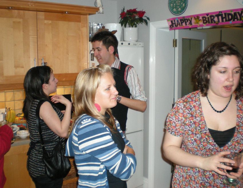
Figure 2: Our mixture-of-trees model encodes topological changes due to viewpoint. Red lines denote springs between pairs
of parts; note there are no closed loops, maintaining the tree property. All trees make use of a common, shared pool of part
templates, which makes learning and inference efficient.
[1] and face.com [2] (the best-performing system on LFW         on global spatial models built on top of local part detectors,
benchmark [3]). We first show results in controlled lab         sometimes known as Constrained Local Models (CLMs)
settings, using the well-known MultiPIE benchmark [16].         [11, 35, 5]. Notably, all such work assumes a densely con-
We definitively outperform past work in all tasks, partic-      nected spatial model, requiring the need for approximate
ularly so for extreme viewpoints. As our results saturate       matching algorithms. By using a tree model, we can use
this benchmark, we introduce a new “in the wild” dataset of     efficient dynamic programming algorithms to find globally
Flickr images annotated with faces, poses, and landmarks.       optimal solutions.
In terms of face detection, our model substantially outper-         From a modeling perspective, our approach is similar to
forms ViolaJones, and is on par with the commercial sys-        those that reason about mixtures of deformable part models
tems above. In terms of pose and landmark estimation, our       [14, 41]. In particular [19] use mixtures of trees for face de-
results dominate even commercial systems. Our results are       tection and [13] use mixtures of trees for landmark estima-
particularly impressive since our model is trained with hun-    tion. Our model simultaneously addresses both with state-
dreds of faces, while commercial systems use up to billions     of-the-art results, in part because it is aggressively trained
of examples [36]. Another result of our analysis is evidence    to do so in a discriminative, max-margin framework. We
of large gap between currently-available academic solutions     also explore part sharing for reducing model size and com-
and commercial systems; we will address this by releasing       putation, as in [37, 29].
open-source software.
                                                                3. Model
2. Related Work
                                                                   Our model is based on mixture of trees with a shared
    As far as we know, no previous work jointly addresses       pool of parts V . We model every facial landmark as a
the tasks of face detection, pose estimation, and landmark      part and use global mixtures to capture topological changes
estimation. However, there is a rich history of all three in    due to viewpoint. We show such mixtures for viewpoint
vision. Space does not allow for a full review; we refer        in Fig.2. We will later show that global mixtures can also
the reader to the recent surveys [42, 27, 40]. We focus on      be used to capture gross deformation changes for a single
methods most related to ours.                                   viewpoint, such as changes in expression.
    Face detection is dominated by discriminatively-trained        Tree structured part model: We write each tree Tm =
scanning window classifiers [33, 22, 28, 18], most ubiqui-      (Vm , Em ) as a linearly-parameterized, tree-structured pic-
tous of which is the Viola Jones detector [38] due its open-    torial structure [41], where m indicates a mixture and Vm ⊆
source implementation in the OpenCV library. Our system         V . Let us write I for an image, and li = (xi , yi ) for the
is also trained discriminatively, but with much less training   pixel location of part i. We score a configuration of parts
data, particularly when compared to commercial systems.         L = {li : i ∈ V } as:
    Pose estimation tends to be addressed in a video scenario
                                                                   S(I, L, m) = Appm (I, L) + Shapem (L) + αm              (1)
[42], or a controlled lab setting that assumes the detection                    X
problem is solved, such as the MultiPIE [16] or FERET [32]        Appm (I, L) =     wim · φ(I, li )                        (2)
benchmarks. Most methods use explicit 3D models [6, 17]                          i∈Vm
or 2D view-based models [31, 10, 21]. We use view-based                            X
                                                                  Shapem (L) =           am    2   m        m    2   m
                                                                                          ij dx + bij dx + cij dy + dij dy
models that share a central pool of parts. From this perspec-
                                                                                 ij∈Em
tive, our approach is similar to aspect-graphs that reason                                                                 (3)
about topological changes between 2D views of an object
[7].                                                            Eqn.2 sums the appearance evidence for placing a template
    Facial landmark estimation dates back to the classic ap-    wim for part i, tuned for mixture m, at location li . We
proaches of Active Appearance Models (AAMs) [9, 26] and         write φ(I, li ) for the feature vector (e.g., HoG descriptor)
elastic graph matching [25, 39]. Recent work has focused        extracted from pixel location li in image I. Eqn.3 scores
the mixture-specific spatial arrangement of parts L, where
dx = xi − xj and dy = yi − yj are the displacement of the
ith part relative to the jth part. Each term in the sum can
be interpreted as a spring that introduces spatial constraints
between a pair of parts, where the parameters (a, b, c, d)
specify the rest location and rigidity of each spring. We
further analyze our shape model in Sec.3.1. Finally, the last
term αm is a scalar bias or “prior” associated with view-
point mixture m.
   Part sharing: Eqn.1 requires a separate template wim                  (a) Tree-based SVM                     (b) AAM
for each mixture/viewpoint m of part i. However, parts            Figure 3: In (a), we show the mean shape µm and defor-
may look consistent across some changes in viewpoint. In          mation modes (eigenvectors of Λm ) learned in our tree-
the extreme cases, a “fully shared” model would use a             structured, max-margin model. In (b), we show the mean
single template for a particular part across all viewpoints,      shape and deformation modes of the full-covariance Gaus-
wim = wi . We explore a continuum between these two               sian shape model used by AAMs. Note we exaggerate the
                         f (m)                                    deformations for visualization purposes. Model (a) captures
extremes, written as wi        , where f (m) is a function that
maps a mixture index (from 1 to M ) to a smaller template         much of the relevant elastic deformation, but produces some
index (from 1 to M 0 ). We explore various values of M 0 : no     unnatural deformations because it lacks loopy spatial con-
sharing (M 0 = M ), sharing across neighboring views, and         straints (e.g., the left corner of the mouth in the lower right
sharing across all views (M 0 = 1).                               plot). Even so, it still outperforms model (b), presumably
                                                                  because it is easier to optimize and allows for joint, dis-
3.1. Shape model                                                  criminative training of part appearance models.
   In this section, we compare our spatial model with a stan-
                                                                  (Vm , Em ) is a tree, the inner maximization can be done ef-
dard joint Gaussian model commonly used in AAMs and
                                                                  ficiently with dynamic programming(DP) [15]. We omit the
CLMs [11, 35]. Because the location variables li in Eqn.3
                                                                  message passing equations for a lack of space.
only appear in linear and quadratic terms, the shape model
                                                                      Computation: The total number of distinct part tem-
can be rewritten as:
                                                                  plates in our vocabulary is M 0 |V |. Assuming each part is of
 Shapem (L) = −(L − µm )T Λm (L − µm ) + constant (4)             dimension D and assuming there exist N candidate part lo-
                                                                  cations, the total cost of evaluating all parts at all locations
where (µ, Λ) are re-parameterizations of the shape model          is O(DN M 0 |V |). Using distance transforms [14], the cost
(a, b, c, d); this is akin to a canonical versus natural pa-      of message passing is O(N M |V |). This makes our over-
rameterization of a Gaussian. In our case, Λm is a block          all model linear in the number of parts and the size of the
sparse precision matrix, with non-zero entries correspond-        image, similar to other models such as AAMs and CLMs.
ing to pairs of parts i, j connected in Em . One can show Λm          Because the distance transform is rather efficient and
is positive semidefinite if and only if the quadratic spring      D is large, the first term (local part score computation) is
terms a and c are negative [34]. This corresponds to a shape      the computational bottleneck. Our fully independent model
score that penalizes configurations of L that deform from         uses M 0 = M , while our fully-shared model uses M 0 = 1,
the ideal shape µm . The eigenvectors of Λm associated with       roughly an order of magnitude difference. In our experi-
the smallest eigenvalues represent modes of deformation as-       mental results, we show that our fully-shared model may
sociated with small penalties. Notably, we discriminatively       still be practically useful as it sacrifices some performance
train (a, b, c, d) (and hence µ and Λ) in a max-margin frame-     for speed. This means our multiview model can run as fast
work. We compare our learned shape models with those              as a single-view model. Moreover, since single-view CLMs
trained generatively with maximum likelihood in Fig.3.            often pre-process their images to compute dense local part
                                                                  scores [35], our multiview model is similar in speed to such
4. Inference                                                      popular approaches but globally-optimizable.

  Inference corresponds to maximizing S(I, L, m) in               5. Learning
Eqn.1 over L and m:
                                                                     To learn our model, we assume a fully-supervised sce-
              S ∗ (I) = max[max S(I, L, m)]                (5)    nario, where we are provided positive images with land-
                          m     L
                                                                  mark and mixture labels, as well as negative images without
Simply enumerate all mixtures, and for each mixture, find         faces. We learn both shape and appearance parameters dis-
the best configuration of parts. Since each mixture Tm =          criminatively using a structured prediction framework. We
first need to estimate the edge structure Em of each mix-
ture. While trees are natural for modeling human bodies
[15, 41, 19], the natural tree structure for facial landmarks
is not clear. We use the Chow-Liu algorithm [8] to find
the maximum likelihood tree structure that best explains
the landmark locations for a given mixture, assuming land-
marks are Gaussian distributed.
Given labeled positive examples {In , Ln , mn } and neg-
ative examples {In }, we will define a structured prediction
objective function similar to one proposed in [41]. To do so,
let’s write zn = {Ln , mn }. Note that the scoring function
Eqn.1 is linear in the part templates w, spring parameters
(a, b, c, d), and mixture biases α. Concatenating these pa-
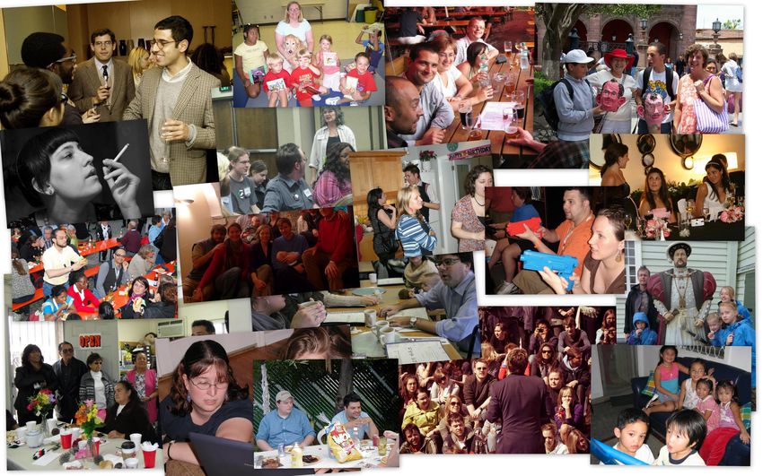
rameters into a single vector β, we can write the score as: Figure 4: Example images from our annotated faces-in-the-
wild (AFW) testing set.
S(I, z) = β · Φ(I, z) (6)
Our annotated face in-the-wild (AFW) testset: To fur-
The vector Φ(I, z) is sparse, with nonzero entries in a single ther evaluate our model, we built an annotated faces in-the-
interval corresponding to mixture m. wild (AFW) dataset from Flickr images (Fig. 4). We ran-
Now we can learn a model of the form: domly sampled images, keeping each that contained at least
one large face. This produced a 205-image dataset with
1 X
arg min β·β+C ξn (7) 468 faces. Images tend to contain cluttered backgrounds
β,ξn ≥0 2 n with large variations in both face viewpoint and appearance
s.t. ∀n ∈ pos β · Φ(In , zn ) ≥ 1 − ξn (aging, sunglasses, make-ups, skin color, expression etc.).
Each face is labeled with a bounding box, 6 landmarks (the
∀n ∈ neg, ∀z β · Φ(In , z) ≤ −1 + ξn
center of eyes, tip of nose, the two corners and center of
∀k ∈ K, βk ≤ 0 mouth) and a discretized viewpoint (−90◦ to 90◦ every 15◦ )
along pitch and yaw directions and (left, center, right) view-
The above constraint states that positive examples should
points along the roll direction. Our dataset differs from sim-
score better than 1 (the margin), while negative examples,
ilar “in-the-wild” collections [20, 3, 23, 5] in its annotation
for all configurations of part positions and mixtures, should
of multiple, non-frontal faces in a single image.
score less than -1. The objective function penalizes vio-
Models: We train our models using 900 positive exam-
lations of these constraints using slack variables ξn . We
ples from MultiPIE, and 1218 negative images from the IN-
write K for the indices of the quadratic spring terms (a, c)
RIAPerson database [12] (which tend to be outdoor scenes
in parameter vector β. The associated negative constraints
that do not contain people). We model each landmark de-
ensure that the shape matrix Λ is positive semidefinite
fined in MultiPIE as a part. There are a total of 99 parts
(Sec.3.1). We solve this problem using the dual coordinate-
across all viewpoints. Each part is represented as a 5 × 5
descent solver in [41], which accepts negativity constraints.
HoG cells with a spatial bin size of 4. We use 13 viewpoints
and 5 expressions limited to frontal viewpoints, yielding a
6. Experimental Results
total of 18 mixtures. For simplicity, we do not enforce sym-
CMU MultiPIE: CMU MultiPIE face dataset [16] con- metry between left/right views.
tains around 750,000 images of 337 people under multi- Sharing: We explore 4 levels of sharing, denoting
ple viewpoints, different expressions and illumination con- each model with the number of distinct templates encoded.
ditions. Facial landmark annotations (68 landmarks for Share-99 (i.e. fully shared model) shares a single tem-
frontal faces (−45◦ to 45◦ ), and 39 landmarks for profile plate for each part across all mixtures. Share-146 shares
faces) are available from the benchmark curators for a rel- templates across only viewpoints with identical topology
atively small subset of images. In our experiments, we use {−45 : 45}, ±{60 : 90}. Share-622 shares templates
900 faces from 13 viewpoints spanning over 180◦ spacing across neighboring viewpoints. Independent-1050 (i.e. in-
at 15◦ for training, and another 900 faces for testing. 300 of dependent model) does not share any templates across any
those faces are frontal, while the remaining 600 are evenly mixtures. We score both the view-specific mixture and part
distributed among the remaining viewpoints. Hence our locations returned by our various models.
training set is considerably smaller than those typically used Computation: Our 4 models tend to have consistent rel-
for training face detectors. Fig. 5 shows example images ative performance across our datasets and evaluations, with
from all the 13 viewpoints with the annotated landmarks. Independent-1050 performing the best, taking roughly 40Figure 5: Example images from MultiPIE with annotated landmarks.
1 1 Results on all faces are summarized in Fig.6a. Our mod-
0.9 0.9
els outperform 2-view Viola-Jones and [22] significantly,
0.8 0.8
Our indep. (ap=88.7%) Our indep. (ap=92.9%) and are only slightly below Google Picasa and face.com.
0.7 Our fully shared (ap=87.2%) 0.7 Our fully shared (ap=92.2%)
Our face model is tuned for large faces such that land-
Precision
precision
DPM,voc−re4 (ap=85.5%) Star model (ap=88.6%)
0.6 0.6
0.5
Star model (ap=77.6%)
Multi. HoG (ap=75.5%) 0.5
DPM,voc−re4 (ap=87.8%)
Multi. HoG (ap=77.4%)
marks are visible. We did another evaluation of all algo-
0.4
Kalal et al.[22] (ap=69.8%)
Google Picasa
0.4
Kalal et al.[22] (ap=68.7%)
Google Picasa
rithms, including baselines, on faces larger than 150 pix-
0.3 face.com 0.3 face.com els in height (a total of 329, or 70% of the faces in AFW).
2−view Viola Jones (OpenCV) 2−view Viola Jones (OpenCV)
0.2
0.2 0.4 0.6 0.8 1
0.2
0.2 0.4 0.6 0.8 1 In this case, our model is on par with Google Picasa and
Recall recall
face.com (Fig.6b). We argue that high-resolution images
(a) all faces (b) large faces only
are rather common given HD video and megapixel cameras.
Figure 6: Precision-recall curves for face detection on our One could define multiresolution variants of our models de-
AFW testset (a) on all faces; (b) on faces larger than 150 × signed for smaller faces [30], but we leave this as future
150 pixels. Our models significantly outperform popular work.
detectors in use and are on par with commercial systems
Fig.6b reveals an interesting progression of performance.
trained with billions of examples, such as Google Picasa
Surprisingly, our rigid multiview HoG baseline outperforms
and face.com.
popular face detectors currently in use, achieving an aver-
age precision (AP) of 77.4%. Adding latent star-structured
seconds per image, while Share-99 performs slightly worse parts, making them supervised, and finally adding tree-
but roughly 10× faster. We present quantitative results later structured relations each contributes to performance, with
in Fig.12. With parallel/cascaded implementations, we be- APs of 87.8%, 88.6%, and 92.9% respectively.
lieve our models could be real-time. Due to space restric- A final point of note is the large gap in performance be-
tions, we mainly present results for these two “extreme” tween current academic solutions and commercial systems.
models in this section. We will address this discrepancy by releasing open-source
In-house baselines: In addition to comparing with nu- software.
merous other systems, we evaluate two restricted versions
of our approach. We define Multi.HoG to be rigid, mul- 6.2. Pose estimation
tiview HoG template detectors, trained on the same data as We compare our approach and baselines with the follow-
our models. We define Star Model to be equivalent to Share- ing: (1) Multiview AAMs: we train an AAM for each view-
99 but defined using a “star” connectivity graph, where all point using the code from [24], and report the view-specific
parts are directly connected to a root nose part. This is sim- model with the smallest reconstruction error on a test image.
ilar to the popular star-based model of [14], but trained in a (2) face.com.
supervised manner given landmark locations.
Fig.8 shows the cumulative error distribution curves on
both datasets. We report the fraction of faces for which the
6.1. Face detection
estimated pose is within some error tolerance. Our indepen-
We show detection results for AFW, since MultiPIE dent model works best, scoring 91.4% when requiring exact
consists of centered faces. We adopt the PASCAL VOC matching, and 99.9% when allowing ±15◦ error tolerance
precision-recall protocol for object detection (requiring on MultiPIE. In general, we find that many methods satu-
50% overlap). We compare our approach and baselines with rate in performance on MultiPIE, originally motivating us
the following: (1) OpenCV frontal + profile Viola-Jones, to collect AFW.
(2) Boosted frontal + profile face detector of [22], (3) De- Unlike on MultiPIE where we assume detections are
formable part model (DPM) [14, 4] trained on same data given (as faces are well centered in image), we evaluate the
as our models, (4) Google Picasa’s face detector, manually performance on AFW in a more realistic manner: we eval-
scored by inspection, (5) face.com’s face detector, which re- uate results on faces found by a given algorithm and count
ports detections, viewpoints, and landmarks. To generate an missed detections as having an infinite error in pose estima-
overly-optimistic multiview detection baseline for (1) and tion. Because AAMs do not have an associated detector, we
(2), we calibrated the frontal and side detectors on the test given them the best-possible initialization with the ground-
set and applied non-maximum suppression (NMS) to gen- truth bounding box on the test set (denoted with an ∗ in
erate a final set of detections. Fig.8b ).Figure 7: Qualitative results of our model on AFW images, tuned for an equal error rate of false positives and missed
detections. We accurately detect faces, estimate pose, and estimate deformations in cluttered, real-world scenes.
Fraction of the num. of testing faces
1 1 (CLM): we use the off-the-shelf code from [35]. This work
0.8 0.8 represents the current state-of-the-art results on landmark
0.6 Multi. AAMs (100.0%) 0.6 Our indep. (81.0%)
estimation in MultiPIE. (3) face.com reports the location
Our indep. (99.9%)
0.4
Our fully shared (76.9%) of a few landmarks, we use 6 as output: eye centers, nose
0.4 Multi. HoG (99.7%) Multi. HoG (74.6%)
Our fully shared (99.4%) Star model (72.9%) tip, mouth corners and center. (4) Oxford facial landmark
0.2 Star model (99.4%) 0.2 face.com (64.3%)
face.com (71.2%) Multi. AAMs (*36.8%)
detector [13] reports 9 facial landmarks: corners of eyes,
0
0
0 10 20 30 0 10 20
Pose estimation error (in degrees)
30 nostrils, nose tip and mouth corners. Both CLM and multi-
Pose estimation error (in degrees)
(a) MultiPIE (b) AFW
view AAMs are carefully initialized using the ground truth
bounding boxes on the test set.
Figure 8: Cumulative error distribution curves for pose es-
Landmark localization error is often normalized with re-
timation. The numbers in the legend are the percentage
spect to the inter-ocular distance [5]; this however, pre-
of faces that are correctly labeled within ±15◦ error tol-
sumes both eyes are visible. This is not always true, and
erance. AAMs are initialized with ground-truth bounding
reveals the bias of current approaches for frontal faces!
boxes (denoted by *). Even so, our independent model
Rather, we normalize pixel error with respect to the face
works best on both MultiPIE and AFW.
size, computed as the mean of height and width.
All curves decrease in performance in AFW (indicating Various algorithms assume different landmark sets; we
the difficulty of the dataset), especially multiview AAMs, train linear regressors to map between these sets. On AFW,
which suggests AAMs generalize poorly to new data. Our we evaluate algorithms using a set of 6 landmarks common
independent model again achieves the best performance, to all formats. On MultiPIE, we use the original 68 land-
correctly labeling 81.0% of the faces within ±15◦ error tol- marks when possible, but evaluate face.com and Oxford us-
erance. In general, our models and Multiview-HoG/Star ing a subset of landmarks they report; note this gives them
baselines perform similarly, and collectively outperform an extra advantage because their localization error tends to
face.com and Multiview AAMs by a large margin. Note be smaller since they output fewer degrees of freedom.
that we don’t penalize false positives for pose estimation; We first evaluate performance on only frontal faces from
our Multiview-HoG/Star baselines would perform worse if MultiPIE in Fig.9a. All baselines perform well, but our in-
we penalized false positives as incorrect pose estimates (be- dependent model (average error of 4.39 pixels/ 2.3% rela-
cause they are worse detectors). Our results are impressive tive error) still outperforms the state-of-the-art CLM model
given the difficulty of this unconstrained data. from [35] (4.75 pixels/ 2.8%). When evaluated on all view
points, we see a performance drop across most baselines,
6.3. Landmark localization
particularly CLMs (Fig.10a). It is worth noting that, since
We compare our approach and baselines with the fol- CLM and Oxford are trained to work on near-frontal faces,
lowing: (1) Multiview AAMs (2) Constrained local model we only evaluate them on faces between −45◦ and 45◦Fraction of the num. of testing faces
Fraction of the num. of testing faces
Fraction of the num. of testing faces
1 1
1 0.8 0.8
Our indep. (99.8%) Our indep. (76.7%)
0.6 0.6
0.8 Our indep. (100.0%) Our fully shared (97.9%) face.com (69.6%)
Star model (96.0%) Our fully shared (63.8%)
Our fully shared (96.7%) 0.4 Multi. AAMs (85.8%) 0.4
Oxford (*57.9%)
0.6 Oxford (*73.5%)
Oxford (94.3%) 0.2 face.com (64.0%) 0.2
Star model (50.2%)
CLM (*24.1%)
0.4 Star model (92.6%) CLM (*47.8%) Multi. AAMs (*15.9%)
0 0
0.05 0.1 0.15 0.05 0.1 0.15
Multi. AAMs (91.2%) Average localization error as fraction of face size Average localization error as fraction of face size
0.2 CLM (90.3%) (a) MultiPIE (b) AFW
face.com (79.6%)
0 Figure 10: Cumulative error distribution curves for land-
0.02 0.04 0.06 0.08 0.1 0.12 0.14 mark localization. The numbers in legend are the percent-
Average localization error as fraction of face size
(a) Localization results on frontal faces from MultiPIE (b)
age of testing faces that have average error below 0.05(5%)
of the face size. (*) denote models which are given an “un-
Figure 9: (a) Cumulative localization error distribution of
fair” advantage, such as hand-initialization or a restriction
the frontal faces from MultiPIE. The numbers in the leg-
to near-frontal faces (described further in the text). Even
end are the percentage of faces whose localization error is
so, our independent model works the best on both MultiPIE
less than .05 (5%) of the face size. Our independent model
and our AFW testset.
produces such a small error for all (100%) faces in the test-
set. (b) Landmark-specific error of our independent model.
Each ellipse denotes the standard deviation of the localiza-
tion errors.
where all frontal landmarks are visible (marked as a ∗ in
Fig.10a). Even given this advantage, our model outper-
forms all baselines by a large margin.
(a) Our model (b) AAM (c) CLM
On AFW (Fig.10b), we again realistically count missed
detections as having a localization error of infinity. We Figure 11: An example AFW image with large mouth de-
report results on large faces where landmarks are clearly formations. AAMs mis-estimate the overall scale in order
visible (which includes 329 face instances in AFW test- to match the mouth correctly. CLM matches the face con-
set). Again, our independent model achieves the best re- tour correctly, but sacrifices accuracy at the nose and mouth.
sult with 76.7% of faces having landmark localization er- Our tree-structured model is flexible enough to capture large
ror below 5% of face size. AAMs and CLM’s accuracy face deformation and yields the lowest localization error.
plunges, which suggests these popular methods don’t gen- 0.029 0.92
Average localization error as fraction of face size
Average localization error
eralize well to in-the-wild images. We gave an advantage to 0.028
Pose estimation accuracy
0.9
AAM, CLM, and Oxford by initializing them with ground
Pose estimation accuracy
0.027
truth bounding boxes on the test set (marked with “∗” in 0.88
Fig.10b). Finally, the large gap between our models and 0.026
0.86
our Star baseline suggests that our tree structure does cap-
0.025
ture useful elastic structure. 0.84
Our models outperform the state-of-the-art on both 0.024
0.82
datasets. We outperform all methods by a large margin on
0.023
MultiPIE. The large performance gap suggest our models 200 400 600 800
Total number of parts in model
1000
maybe overfitting to the lab conditions of MultiPIE; this in Figure 12: We show how different levels of sharing (as de-
turn suggests they may do even better if trained on “in-the- scribed at the beginning of Sec.6) affect the performance of
wild” training data similar to AFW. Our model even outper- our models on MultiPIE. We simultaneously plot localiza-
forms commercial systems such as face.com. This result is tion error in red (lower is better) and pose estimation ac-
surprising since our model is only trained with 900 faces, curacy in blue (higher is better), where poses need to be
while the latter appears to be trained using billions of faces predicted with zero error tolerance. The larger number of
[36]. part templates indicate less sharing. The fully independent
Fig.9b plots the landmark specific localization error of model works best on both tasks.
our independent model on frontal faces from MultiPIE.
Note that the errors around the mouth are asymmetric, due still generates fairly accurate localizations even compared
to the asymmetric spatial connectivity required by a tree- to baselines encoding such dense spatial constraints - we
structure. This suggests our model may still benefit from show an example AFW image with large mouth deforma-
additional loopy spatial constraints. However, our model tions in Fig.11.Conclusion: We present a unified model for face de- [20] V. Jain and E. Learned-Miller. Fddb: A benchmark for face
tection, pose estimation and landmark localization using a detection in unconstrained settings. Technical Report UM-
mixture of trees with a shared pool of parts. Our tree models CS-2010-009, UMass, Amherst, 2010. 4
are surprisingly effective in capturing global elastic defor- [21] M. Jones and P. Viola. Fast multi-view face detection. In
mation, while being easy to optimize. Our model outper- CVPR 2003. 2
[22] Z. Kalal, J. Matas, and K. Mikolajczyk. Weighted sampling
forms state-of-the-art methods, including large-scale com-
for large-scale boosting. In BMVC 2008. 2, 5
mercial systems, on all three tasks under both constrained
[23] M. Köstinger, P. Wohlhart, P. M. Roth, and H. Bischof. An-
and in-the-wild environments. To demonstrate the latter, we notated facial landmarks in the wild: A large-scale, real-
present a new annotated dataset which we hope will spur world database for facial landmark localization. In First
further progress. IEEE International Workshop on Benchmarking Facial Im-
Acknowledgements: Funding for this research was pro- age Analysis Technologies 2011. 4
vided by NSF Grant 0954083, ONR-MURI Grant N00014- [24] D.-J. Kroon. Active shape model and active ap-
10-1-0933, and support from Intel. pearance model. http://www.mathworks.com/
matlabcentral/fileexchange/26706. 5
References [25] T. Leung, M. Burl, and P. Perona. Finding faces in cluttered
[1] http://picasa.google.com/. 2 scenes using random labeled graph matching. In ICCV 1995.
2
[2] http://face.com/. 2
[26] I. Matthews and S. Baker. Active appearance models revis-
[3] http://vis-www.cs.umass.edu/lfw/results.
ited. IJCV, 60(2):135–164, 2004. 2
html. 2, 4
[27] E. Murphy-Chutorian and M. Trivedi. Head pose estimation
[4] http://www.cs.brown.edu/˜pff/latent/
in computer vision: A survey. IEEE TPAMI, 2009. 2
voc-release4.tgz. 5
[28] M. Osadchy, Y. L. Cun, and M. L. Miller. Synergistic face
[5] P. N. Belhumeur, D. W. Jacobs, D. J. Kriegman, and N. Ku- detection and pose estimation with energy-based models.
mar. Localizing parts of faces using a consensus of exem- JMLR, 2007. 2
plars. In CVPR 2011. 2, 4, 6 [29] P. Ott and M. Everingham. Shared parts for deformable part-
[6] V. Blanz and T. Vetter. Face recognition based on fitting a 3d based models. In CVPR 2011. 2
morphable model. IEEE TPAMI, 2003. 2 [30] D. Park, D. Ramanan, and C. Fowlkes. Multiresolution mod-
[7] K. Bowyer and C. Dyer. Aspect graphs: An introduction and els for object detection. In ECCV 2010. 5
survey of recent results. International Journal of Imaging [31] A. Pentland, B. Moghaddam, and T. Starner. View-based and
Systems and Technology, 1990. 2 modular eigenspaces for face recognition. In CVPR 1994. 2
[8] C. Chow and C. Liu. Approximating discrete probability [32] P. Phillips, H. Moon, S. Rizvi, and P. Rauss. The feret eval-
distributions with dependence trees. IEEE TIT, 1968. 4 uation methodology for face-recognition algorithms. IEEE
[9] T. Cootes, G. Edwards, and C. Taylor. Active appearance TPAMI, 2000. 2
models. IEEE TPAMI, 2001. 1, 2 [33] H. Rowley, S. Baluja, and T. Kanade. Neural network-based
[10] T. Cootes, K. Walker, and C. Taylor. View-based active ap- face detection. IEEE TPAMI, 1998. 2
pearance models. In IEEE FG 2000, 2000. 2 [34] H. Rue and L. Held. Gaussian Markov random fields: theory
[11] D. Cristinacce and T. Cootes. Feature detection and tracking and applications, volume 104. Chapman & Hall, 2005. 3
with constrained local models. In BMVC 2006. 2, 3 [35] J. Saragih, S. Lucey, and J. Cohn. Deformable model fitting
[12] N. Dalal and B. Triggs. Histograms of oriented gradients for by regularized landmark mean-shift. IJCV, 2011. 2, 3, 6
human detection. In CVPR 2005. 4 [36] Y. Taigman and L. Wolf. Leveraging Billions of Faces
[13] M. Everingham, J. Sivic, and A. Zisserman. “Hello! My to Overcome Performance Barriers in Unconstrained Face
name is... Buffy” – automatic naming of characters in TV Recognition. ArXiv e-prints, Aug. 2011. 2, 7
video. In BMVC 2006. 2, 6 [37] A. Torralba, K. P. Murphy, and W. T. Freeman. Sharing vi-
[14] P. Felzenszwalb, R. Girshick, D. McAllester, and D. Ra- sual features for multiclass and multiview object detection.
manan. Object detection with discriminatively trained part- IEEE TPAMI. 2
based models. IEEE TPAMI, 2009. 2, 3, 5 [38] P. Viola and M. J. Jones. Robust real-time face detection.
[15] P. F. Felzenszwalb and D. P. Huttenlocher. Pictorial struc- IJCV, 2004. 2
tures for object recognition. IJCV, 2005. 3, 4 [39] L. Wiskott, J.-M. Fellous, N. Kuiger, and C. von der Mals-
[16] R. Gross, I. Matthews, J. Cohn, T. Kanade, and S. Baker. burg. Face recognition by elastic bunch graph matching.
Multi-pie. Image and Vision Computing, 2010. 2, 4 IEEE TPAMI, Jul 1997. 1, 2
[17] L. Gu and T. Kanade. 3d alignment of face in a single image. [40] M.-H. Yang, D. Kriegman, and N. Ahuja. Detecting faces in
In CVPR 2006. 2 images: a survey. IEEE TPAMI, 2002. 2
[18] B. Heisele, T. Serre, and T. Poggio. A Component-based [41] Y. Yang and D. Ramanan. Articulated pose estimation using
Framework for Face Detection and Identification. IJCV, flexible mixtures of parts. In CVPR 2011, 2011. 2, 4
2007. 2 [42] W. Zhao, R. Chellappa, P. Phillips, and A. Rosenfeld. Face
[19] S. Ioffe and D. Forsyth. Mixtures of trees for object recogni- recognition: A literature survey. ACM Computing Surveys,
tion. In CVPR 2001. 2, 4 2003. 1, 2You can also read