Towards model discovery with reinforcement learning - Fluid ...

Center for Turbulence Research
Annual Research Briefs 2019

     Towards model discovery with reinforcement
                      learning
                        By A. Lozano-Durán† & M. Bassenne†‡

1. Motivation and objectives
   5 to 0. This is the score by which AlphaStar–a computer program developed by the
artificial intelligence (AI) company DeepMind–beat a top professional player in Starcraft
II, one of the most complex video games to date (Vinyals et al. 2019). This accomplish-
ment tops the list of sophisticated human tasks at which AI is now performing at a
human or superhuman level (Perrault et al. 2019), and enlarges the previous body of
achievements in game playing (Silver et al. 2017, 2018) and in other tasks, e.g. medical
diagnoses (Esteva et al. 2017; Raumviboonsuk et al. 2019; Nagpal et al. 2019).
   Our focus is on computational modeling, which is of paramount importance to the in-
vestigation of many natural and industrial processes. Reduced-order models alleviate the
computational intractability frequently associated with solving the exact mathematical
description of the full-scale dynamics of complex systems. The motivation of this study
is to leverage recent breakthroughs in AI research to unlock novel solutions to important
scientific problems encountered in computational science. Following the post-game con-
fession of the human player defeated by AlphaStar: “The agent demonstrated strategies
I hadn’t thought of before, which means there may still be new ways of playing the game
that we havent fully explored yet” (Vinyals et al. 2019), we inquire current AI potential
to discover scientifically rooted models that are free of human bias for computational
physics applications.
   Traditional reduced-order modeling approaches are rooted in physical principles, math-
ematics, and phenomenological understanding, all of which are important contributors
to the human interpretability of the models. However these strategies can be limited
by the difficulty of formalizing an accurate reduced-order model, even when the exact
governing equations are known. A notorious example in fluid mechanics is turbulence:
the flow is accurately described in detail by the Navier-Stokes equations; however, closed
equations for the large-scale quantities remain unknown, despite their expected simpler
dynamics. The work by Jiménez (2020) discusses in more extent the role of computers
in the development of turbulence theories and models.
   To address the human intelligence limitations in discovering reduced-order models, we
propose to supplement human thinking with artificial intelligence. Our work shares the
goal of a growing body of literature on data-driven discovery of differential equations,
which aims at substituting or combining traditional modeling strategies with the appli-
cation of modern machine learning algorithms to experimental or high-fidelity simulation
data (see Brunton et al. 2019, for a review on machine learning and fluid mechanics).
Early work used symbolic regression and evolutionary algorithms to determine the dy-
namical model that best describes experimental data (Bongard & Lipson 2007; Schmidt
   † Authors contributed equally.
   ‡ Laboratory of Artificial Intelligence in Medicine and Biomedical Physics, Stanford Univer-
sity, CA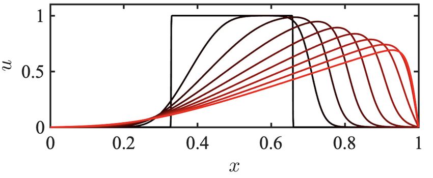

Lozano-Durán & Bassenne
& Lipson 2009). An alternative, less costly approach consists of selecting candidate terms
in a predefined dictionary of simple functions using sparse regression (Brunton et al. 2016;
Rudy et al. 2017; Schaeffer 2017; Wu & Zhang 2019). Raissi et al. (2017) and Raissi &
Karniadakis (2018) use Gaussian processes to learn unknown scalar parameters in an
otherwise known partial differential equation. A recent method exploits the connection
between neural networks and differential equations (Chen et al. 2018) to simultaneously
learn the hidden form of an equation and its numerical discretization (Long et al. 2018,
2019). Atkinson et al. (2019) use genetic programming to learn free-form differential
equations. The closest work to ours in spirit is that of Lee et al. (2019), in which the
authors identify coarse-scale dynamics from microscopic observations by combining Gaus-
sian processes, artificial neural networks, and diffusion maps. It is also worth mentioning
the distinct yet complementary work by Bar-Sinai et al. (2019), which deals with the use
of supervised learning to learn discretization schemes.
   Our three-pronged strategy consists of learning (i) models expressed in analytical form,
(ii) which are evaluated a posteriori, and (iii) using exclusively integral quantities from
the reference solution as prior knowledge. In point (i), we pursue interpretable models
expressed symbolically as opposed to black-box neural networks, the latter only being
used during learning to efficiently parameterize the large search space of possible models.
In point (ii), learned models are dynamically evaluated a posteriori in the computa-
tional solver instead of based on a priori information from preprocessed high-fidelity
data, thereby accounting for the specificity of the solver at hand such as its numerics.
Finally in point (iii), the exploration of new models is solely guided by predefined in-
tegral quantities, e.g., averaged quantities of engineering interest in Reynolds-averaged
or large-eddy simulations (LES). This also enables the assimilation of sparse data from
experimental measurements, which usually provide an averaged large-scale description
of the system rather than a detailed small-scale description. We use a coupled deep re-
inforcement learning framework and computational solver to concurrently achieve these
objectives. The combination of reinforcement learning with objectives (i), (ii) and (iii)
differentiate our work from previous modeling attempts based on machine learning.
   The rest of this brief is organized as follows. In Section 2, we provide a high-level
description of the model discovery framework with reinforcement learning. In Section 3,
the method is detailed for the application of discovering missing terms in differential
equations. An elementary instantiation of the method is described that discovers missing
terms in the Burgers’ equation. Concluding remarks are offered in Section 4.

2. Model Discovery with Reinforcement Learning (MDRL)
                    2.1. Offload human thinking by machine learning
The purpose of modeling is to devise a computational strategy to achieve a prescribed
engineering or physical goal, as depicted in Figure 1. For example, we may search a
subgrid-scale (SGS) model for LES (strategy) that can accurately predict the average
mass flow in a pipe (goal). While it is natural that determining the goal is a completely
human oriented task, as we aim to solve a problem of our own interest, there is no obvious
reason why this should be the case for the strategy.
  Traditionally, as shown in Figure 1(a), finding a modeling strategy heavily relies on
human thinking, which encompasses phenomenological understanding, physical insights,
and mathematical derivations, among others. Deriving a model is typically an iterative
process that involves testing and refining ideas sequentially. Although strategies devised

Towards model discovery with reinforcement learning

                               Model                                                Model
            Goal                                                   Goal

                               Feedback                                             Feedback

Scientist          Scientist           Computational   Scientist           Neural           Computational
                                          Solver                          Network              Solver

                        (a)                                                  (b)
Figure 1. Iterative computational modeling process based on human intelligence (a) alone
and (b) aided by artificial intelligence to offload human thinking during the iterative modeling
process. In approach (b), neural network parameterizations allow to efficiently explore a large
number of models with minimum bias. Blue colored elements highlight differences between both
approaches.

by human intelligence alone have shown success in the past, many earlier models can be
substantially improved, and many remain to be found. Current modeling strategies may
be hindered by the limits of human cognition, for example by a researcher’s preconceived
ideas and biases. In a sense, we have a vast knowledge about traditional models but very
limited idea about what we really seek: breakthrough models. This often constrains us to
exploit prior knowledge for convenience more than we explore innovative ideas. Following
the example in the previous paragraph, we can constrain the functional form of the SGS
model in LES to be an eddy viscosity model and focus on the eddy viscosity parameter
alone. This approach certainly facilitates the strategy search as the space of all possible
models is often too large for researchers to exhaustively explore all of them. However,
it is perhaps at the expense of constraining the final strategy to a suboptimal solution
from the beginning of the modeling process.
   Ideally, we would like to offload all human thinking of strategies to artificial intelligence
to efficiently explore the phase space of models with minimum human bias, as sketched
in Figure 1(b). Following the previous example, our goal is to predict the average mass
flow, but whether we use LES or another computational approach, broadly defined, needs
not be decided by a human, but instead by an artificial intelligent agent. To automate
the full strategy process pertains to the bigger quest of general artificial intelligence
(Goertzel & Pennachin 2007). The aim of the present preliminary study is more modest.
Yet, it is our premise that current machine learning tools already enable to automate a
significant portion of the modeling strategy search. In the previous example where we
seek a model to estimate the pipe mass flow, we might constrain the strategy to employ
a LES framework, then use the artificial intelligent agent to specifically find the SGS
model.

            2.2. Hybrid human/machine method based on reinforcement learning
We pursue a method in which a reinforcement learning (RL) agent is used to partially
replace human thinking in devising strategies. RL emulates how humans naturally learn
and, similarly, how scientists iterate during the modeling process. In particular, we draw
inspiration from the recent success of RL in achieving superhuman performance across a
number of tasks such as controlling robots (OpenAI et al. 2018) or playing complicated
strategy games (Silver et al. 2017, 2018; Vinyals et al. 2019).
   RL consists of training a software agent to take actions that maximize a predefined
notion of cumulative reward in a given environment (Sutton & Barto 2018): the RL
agent selects an action based on its current policy and state, and sends the action to
the environment. After the action is taken, the RL agent receives a reward from the

Lozano-Durán & Bassenne
                                          ACTION
                                          (Model)

                       AGENT                          ENVIRONMENT
             (Scientist/Neural network)             (Computational solver)

                                        REWARD
                                    (Averaged accuracy)
 Figure 2. Schematic representation of MDRL based on a reinforcement learning framework
                       that mimics the scientific modeling process.

environment depending on the success in achieving a prescribed goal. The agent updates
the policy parameters based on the taken action and the reward received. This process
is continuously repeated during training, allowing the agent to learn an optimal policy
for the given environment and reward signal.
   The MDRL methodology proposed here relies on a tailored RL framework that mimics
the scientific modeling process, as illustrated in Figure 2. MDRL consists of training a
software scientist (agent with a given policy) to iteratively search for the optimal strategy
or model (action) that maximizes the prescribed goals (reward) obtained by using the
model in a computational solver (environment). As the state typically encountered in
RL does not play a role here, MDRL may be considered an example of the multi-armed
bandit problem (Sutton & Barto 2018).

3. Application of MDRL for analytical model discovery
  Hereafter, we narrow the term model to refer to mathematical expressions. Instead
of hand-designing new models from scratch, we design a RL agent that searches for
analytical formulas among the space of known primitive functions. In Section 3.1, we
describe how MDRL automates the process of discovering models in analytical form.
An elementary instantiation of the method is presented in Section 3.2, where MDRL is
utilized to efficiently discover missing terms in the Burgers’ equation.

                              3.1. Description of the method
The workflow of MDRL for analytical model discovery is illustrated in Figure 3. The
steps are summarized as follows:
   (1) A random model generator (RMG) is the agent that outputs mathematical expres-
sions (actions) with a given probability distribution, similarly to a sequence of numbers
generated by a random number generator. The RMG comprises a computational graph
to encode mathematical formulas of arbitrary complexity in a particular domain-specific
language (DSL). The probabilities defining the RMG are parameterized as a neural net-
work, which represents the policy of the RL agent.
   (2) A set of models is sampled from the RMG and decoded into their corresponding
mathematical expressions (M in Figure 3).
   (3) The sampled models are evaluated in the real environment using a computational
solver.
   (4) The reward signal is calculated based on the prescribed goals and used to optimize
the parameters (probabilities) of the RMG via a particular RL algorithm.

Towards model discovery with reinforcement learning

Figure 3. Schematic of the Model Discovery with Reinforcement Learning (MDRL) applied
to the analytical discovery of models. A mathematical expression for the model is discovered
following the requirements imposed as a “reward”. For example, a typical reward would be
a measure of global accuracy. Additional requirements can be enforced such as dimensional
consistency, simplicity of the model, Galilean invariance, etc.

The process described in Steps 1 to 4 is repeated until a convergence criterion is satisfied.

   The framework provided by MDRL has the unique feature of allowing the researcher
to focus on the intellectually relevant properties of the model without the burden of spec-
ifying a predetermined analytical form. The final outcome is an equation modeling the
phenomena of interest that can be inspected and interpreted, unlike other widespread ap-
proaches based on neural networks. Our method generates a mathematical equation, but
could be similarly applied to generate symbolic expressions for numerical discretizations.
   We discuss next some of the components of MDRL for analytical model discovery.
   Domain-specific language: A Domain-specific language (DSL) is used to represent
mathematical expressions in a form that is compatible with the reinforcement learn-
ing task. The purpose of the DSL is to map models to actions in the RL framework.
Mathematical expressions can be generally represented as computational graphs, where
the nodes correspond to operations or variables. Compatible representations of these
computational graphs can employ sequence-like or tree-like structures (Bello et al. 2017;
Luo & Liu 2018; Lample & Charton 2019), with varying degree of nesting depending on
the requested complexity of the sought-after mathematical expression. It is important
to remark that the search space is not restricted to elementary physical processes as
the DSL allows for complex combinations of elementary operations to build new ones,
similarly as to how with a few letters one can write a large number of words. The choice
of the DSL plays an important role as it conditions the search space and therefore the
learning process.
   Random model generator as a neural network: The key insight that enables the RL
agent to efficiently learn a model in the vast search space is to implicitly parameterize
the latter using a neural network. The RMG (agent) employs a stochastic policy network
to decide what models (actions) to sample. Actions are sampled according to a multi-
dimensional probability distribution πθ , where π is the neural network policy and θ its
parameters. The objective is to train the RMG to output models with increasing accu-

Lozano-Durán & Bassenne

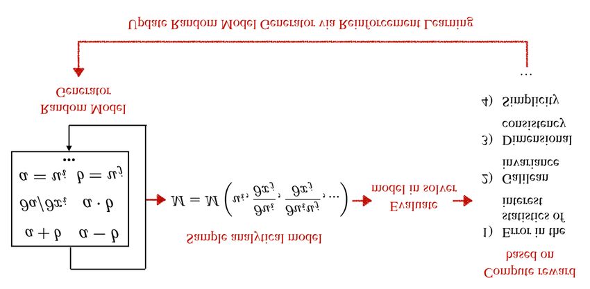
                Figure 4. History of the solution to the Burgers’ equation.

racy by learning a probability distribution function πθ that maximizes the probability of
sampling accurate models. The RL training objective can be formulated as maximizing
                                  J(θ) = Ea∼πθ (·) [R(a)],                            (3.1)
where R(a) is the averaged accuracy (reward) of an action a (≡ M ), sampled according
to a probability distribution πθ . The objective is to maximize the expected performance
J(θ) obtained when sampling a model from the probability distribution outputted by
the policy. This is achieved by gradient ascending on the performance objective J, using
policy gradient algorithms for example.
   A distributed training scheme can be employed to speed up the training of the RMG.
As the model evaluation is generally the most time-consuming bottleneck, it is desirable
to evaluate generated models in parallel on distributed CPUs. In this manner, at each
iteration, the RMG samples a batch of models that are all run simultaneously and later
combined to update the probabilities of the RMG.

           3.2. Example: discovering missing terms in the Burgers’ equation
We apply the scheme proposed in Section 3.1 to discover the analytic form of missing
terms in a partial differential equation. We choose the Burgers’ equation as representative
of the key features of a simple fluid system,
                                  ∂u      ∂u   ∂2u
                                     = −u    +ν 2,                                    (3.2)
                                  ∂t      ∂x   ∂x
where u denotes velocity, x and t are the spatial and temporal coordinates, respec-
tively, and ν = 0.01 is the viscosity. We simulate Eq. (3.2) using as a initial condition
a rectangular signal. The equation is integrated from t = 0 to t = 0.8 using a fourth-
order Runge-Kutta scheme for time-stepping and a fourth-order central finite difference
scheme for approximating the spatial derivatives with 1000 points uniformly distributed
in x. The velocity profile is plotted at various time instants in Figure 4.
   The problem is formulated by re-arranging Eq. (3.2) as
                               ∂u   1 ∂u    ∂2u
                                  =− u   + ν 2 + M,                                   (3.3)
                               ∂t   2 ∂x    ∂x
where M is an unknown mathematical expression that we aim to discover using the
MDRL framework proposed in Figure 3. For each model M = M (u, x, t, ∂u/∂x, ...) sam-

Towards model discovery with reinforcement learning
pled by the RMG, we compute the associated reward as
                                                 1                       ǫ−1
                      Ri =                                             +     ,           (3.4)
                             ||uexact (x, T ) − umodel,i (x, T )|| + ǫ    n
where || · || is the L2 -norm, uexact is the exact solution at t = T = 0.8, umodel,i is the
solution for the i-th model at t = T = 0.8, n is the number of terms in M (for example
n = 2 for M = u2 + ∂u/∂x), and ǫ = 0.1. The first term in R evaluates the accuracy of
the model, whereas the second term penalizes the model based on its complexity (number
of terms). In each iteration P
                             of the RL process, the RMG samples m = 100 models, which
results in the total reward m   i=1 Ri . The reward is then used to improve the RMG.
   We discuss next the implementation of the RMG and the neural network architecture
for the RL agent used in this particular example. Both the proper design of the RMG
agent along with the choice of the optimization method plays a major role in the success
of the proposed methodology. The specific choices made here have shown acceptable
performance, but we do not imply that these are optimal or extensible to other cases.
   For the computational graph representation of M , we follow a DSL methodology similar
to that used by Bello et al. (2017). Models M are formed by combining operands, unary
functions, and binary functions. Each group is composed of a few elementary elements:
   • Operands: u, x, t, and integers c from 1 to 100 and the reciprocals 1/c.
   • Unary functions: (·) (identity), −(·) (sign flip), exp(·), log(| · |), sin(·), cos(·), and
∂(·)/∂x (differentiation).
   • Binary functions: + (addition), − (subtraction), × (multiplication), and / (division).
Formulas with an arbitrary number of terms are generated following a recursive scheme
similar to the one depicted in Figure 3. The details of the specific DSL strategy adopted
here can be cumbersome. They are not emphasized as they are merely designed for the
particular showcase discussed in this example. Further details regarding the unique and
efficient representation of analytical formulas using computational graphs can be found
in Bello et al. (2017), Luo & Liu (2018), and Lample & Charton (2019).
   We use Deep Deterministic Policy Gradients (DDPG) (Lillicrap et al. 2016) as the
network architecture for the RL agent. The DDPG actor-critic algorithm is well suited for
problems with continuous action spaces, which we assimilate to the probabilities required
for the RMG in the current setting. The DDPG is implemented using MATLAB (R2019a,
The MathWorks Inc.) with default parameters. The actor (RMG agent) is a multilayer
perceptron with two blocks, each with 5 fully connected hidden layers. Rectified linear
units and sigmoid activations are used in the first and second blocks, respectively. The
critic neural network is a multilayer perceptron with 5 fully connected hidden layers with
rectified linear units as activation functions. Each layer contains roughly one hundred
neurons.
   The probability of finding the exact solution, M = −1/2 u ∂u/∂x, during the learning
process is shown in Figure 5. The result is obtained by performing 100 independent
learning processes starting from scratch (RMG with uniform probability distribution).
After approximately 220 iterations, the probability of discovering the exact solution is
99%. Our results can be compared with a random search approach, i.e. attempting to
discover the model M according to a fixed RMG with uniform probability distribution.
The latter typically requires more than O(109 ) iterations to find the exact solution.
Note that this random search approach was possible in the present example, but for
cases with a vastly larger phase space, as in real-world applications, the random search
becomes intractable and is likely to fail in finding an accurate model. Hence, the results

Lozano-Durán & Bassenne
             100

              50

                0
                    0    50     100     150     200     250      300     350     400

Figure 5. The probability of finding the exact solution for the missing term, M = −1/2 u ∂u/∂x,
as a function of the iteration number. The dashed line represents 100% probability of finding
the exact solution.

suggest that MDRL is successful in detecting useful patterns in mathematical expressions
and thereby speeds up the search process.

4. Conclusions
   In this preliminary work, we discuss a paradigm for discovering reduced-order com-
putational models assisted by deep reinforcement learning. Our main premise is that
state-of-the-art artificial intelligence algorithms enable to offload a significant portion of
human thinking during the modeling process, in a manner that differs from the conven-
tional approaches followed up to date.
   We have first divided the modeling process into two broad tasks: defining goals and
searching for strategies. Goals essentially summarize the problem we pursue to solve,
whereas strategies denote practical solutions employed to achieve these goals. Within the
framework discussed here, we have argued that defining goals ought to remain in the realm
of human thinking, as we aim to solve a problem of our interest. In contrast, strategies
are mere practical means to achieve these goals. Thus we have advocated for a flexible
methodology that intelligently search for optimal strategies while reducing scientists’
biases during the search process. We deemed the latter necessary to prevent misleading
preconceptions from hindering our potential to discover ground-breaking models.
   In this brief, we presented the main ideas behind a hybrid human/AI method for model
discovery by reinforcement learning (MDRL). The approach consists of learning models
that are evaluated a posteriori using exclusively integral quantities from the reference
solution as prior knowledge. This allows the use of a wide source of averaged/large-scale
computational and experimental data. The workflow is as follows. The scientist sets
the goals, which defines the reward for the reinforcement learning agent. An intelligent
agent devises a strategy that ultimately results in a model candidate. The model is
evaluated in the real environment. The resulting performance, as measured by the reward,
is fed back into the reinforcement learning agent that learns from that experience. The
process is repeated until the model proposed by the agent meets the prescribed accuracy
requirements. In the long term, it would be desirable to offload all human thinking of
strategies to artificial intelligence. In this preliminary work, only a portion of the strategy
is discovered by machine learning.
   We have detailed the scheme above by combining MDRL with computational graphs
to learn analytical mathematical expressions. The approach comprises two components: a
random model generator (agent) that generates symbolic expressions (models) according

Towards model discovery with reinforcement learning
to a parameterized probability distribution, and a reinforcement learning algorithm that
updates the parameters of the model generator. At each iteration, the agent learns to
output better models by updating its parameters based on the error incurred by the
tested models. As an example, we have applied MDRL to discovering missing terms in
the Burgers’ equation. This simple yet meaningful example shows how our approach
retrieves the exact analytical missing term in the equation and outperforms a blind
random search by several orders of magnitude in terms of computational cost.
   Although the main motivating examples in this brief pertain to the field of fluid me-
chanics, the MDRL method can be applied to devising computational models or discov-
ering theories in other engineering and scientific disciplines. Finally, the present brief
should be understood as a statement of concepts and ideas, rather than a collection of
best practices regarding the particular implementations (computational graphs, neural
network architectures, etc.) of the MDRL for general problems. Refinement and further
assessment of the method are currently investigated and will be discussed in future work.

Acknowledgments
 A.L.-D. acknowledges the support of NASA under grant No. NNX15AU93A and of
ONR under grant No. N00014-16-S-BA10. We thank Irwan Bello for useful discussions.
We also thank Jane Bae for her comments on the brief.

                                    REFERENCES
Atkinson, S., Subber, W., Wang, L., Khan, G., Hawi, P. & Ghanem, R. 2019
    Data-driven discovery of free-form governing differential equations. In Advances in
    neural information processing systems (Second Workshop on Machine Learning and
    the Physical Sciences).
Bar-Sinai, Y., Hoyer, S., Hickey, J. & Brenner, M. P. 2019 Learning data-driven
    discretizations for partial differential equations. Proc. Natl. Acad. Sci. 116, 15344–
    15349.
Bello, I., Zoph, B., Vasudevan, V. & Le, Q. V. 2017 Neural optimizer search
    with reinforcement learning. In Proceedings of the 34th International Conference on
    Machine Learning-Volume 70 , pp. 459–468. JMLR.org.
Bongard, J. & Lipson, H. 2007 Automated reverse engineering of nonlinear dynamical
    systems. Proc. Natl. Acad. Sci. 104, 9943–9948.
Brunton, S. L., Noack, B. R. & Koumoutsakos, P. 2019 Machine learning for
    fluid mechanics. Annu. Rev. Fluid Mech. 52.
Brunton, S. L., Proctor, J. L. & Kutz, J. N. 2016 Discovering governing equations
    from data by sparse identification of nonlinear dynamical systems. Proc. Natl. Acad.
    Sci. 113, 3932–3937.
Chen, T. Q., Rubanova, Y., Bettencourt, J. & Duvenaud, D. K. 2018 Neural
    ordinary differential equations. In Adv. Neural Inf. Process Syst., pp. 6571–6583.
Esteva, A., Kuprel, B., Novoa, R. A., Ko, J., Swetter, S. M., Blau, H. M. &
    Thrun, S. 2017 Dermatologist-level classification of skin cancer with deep neural
    networks. Nature 542, 115.
Goertzel, B. & Pennachin, C. 2007 Artificial general intelligence, vol. 2. Springer.
Jiménez, J. 2020 Computers and turbulence. Eur. J. Mech. B-Fluid 79, 1–11.
Lample, G. & Charton, F. 2019 Deep learning for symbolic mathematics.

Lozano-Durán & Bassenne
Lee, S., Kooshkbaghi, M., Spiliotis, K., Siettos, C. I. & Kevrekidis, I. G. 2019
    Coarse-scale PDEs from fine-scale observations via machine learning. arXiv preprint
    arXiv:1909.05707 .
Lillicrap, T. P., Hunt, J. J., Pritzel, A., Heess, N., Erez, T., Tassa, Y.,
    Silver, D. & Wierstra, D. 2016 Continuous control with deep reinforcement
    learning. In ICLR (ed. Y. Bengio & Y. LeCun).
Long, Z., Lu, Y. & Dong, B. 2019 PDE-Net 2.0: Learning PDEs from data with a
    numeric-symbolic hybrid deep network. J. Comput. Phys. 399, 108925.
Long, Z., Lu, Y., Ma, X. & Dong, B. 2018 PDE-Net: Learning PDEs from Data. In
    International Conference on Machine Learning, pp. 3214–3222.
Luo, M. & Liu, L. 2018 Automatic derivation of formulas using reforcement learning.
    arXiv preprint arXiv:1808.04946 .
Nagpal, K., Foote, D., Liu, Y., Chen, P.-H. C., Wulczyn, E., Tan, F., Olson,
    N., Smith, J. L., Mohtashamian, A., Wren, J. H. et al. 2019 Development and
    validation of a deep learning algorithm for improving gleason scoring of prostate
    cancer. NPJ Digit. Med. 2, 48.
OpenAI, Andrychowicz, M., Baker, B., Chociej, M., Józefowicz, R., Mc-
    Grew, B., Pachocki, J. W., Pachocki, J., Petron, A., Plappert, M.,
    Powell, G., Ray, A., Schneider, J., Sidor, S., Tobin, J., Welinder, P.,
    Weng, L. & Zaremba, W. 2018 Learning dexterous in-hand manipulation. CoRR
    abs/1808.00177.
Perrault, R., Shoham, Y., Brynjolfsson, E., Clark, J., Etchemendy, J.,
    Grosz, B., Lyons, T., Manyika, J. & Niebles, S. M. J. C. 2019 The AI Index
    2019 Annual Report. AI Index Steering Committee, Human-Centered AI Institute,
    Stanford University, Stanford, CA.
Raissi, M. & Karniadakis, G. E. 2018 Hidden physics models: Machine learning of
    nonlinear partial differential equations. J. Comput. Phys 357, 125–141.
Raissi, M., Perdikaris, P. & Karniadakis, G. E. 2017 Physics informed deep learn-
    ing (part ii): Data-driven discovery of nonlinear partial differential equations. arXiv
    preprint arXiv:1711.10566 .
Raumviboonsuk, P., Krause, J., Chotcomwongse, P., Sayres, R., Raman, R.,
    Widner, K., Campana, B. J., Phene, S., Hemarat, K., Tadarati, M. et al.
    2019 Deep learning versus human graders for classifying diabetic retinopathy severity
    in a nationwide screening program. NPJ Digit. Med. 2, 25.
Rudy, S. H., Brunton, S. L., Proctor, J. L. & Kutz, J. N. 2017 Data-driven
    discovery of partial differential equations. Sci. Adv. 3, e1602614.
Schaeffer, H. 2017 Learning partial differential equations via data discovery and sparse
    optimization. Proc. R. Soc. Lond. A 473, 20160446.
Schmidt, M. & Lipson, H. 2009 Distilling free-form natural laws from experimental
    data. Science 324, 81–85.
Silver, D., Hubert, T., Schrittwieser, J., Antonoglou, I., Lai, M., Guez,
    A., Lanctot, M., Sifre, L., Kumaran, D., Graepel, T. et al. 2018 A general
    reinforcement learning algorithm that masters chess, shogi, and go through self-play.
    Science 362, 1140–1144.
Silver, D., Schrittwieser, J., Simonyan, K., Antonoglou, I., Huang, A., Guez,
    A., Hubert, T., Baker, L., Lai, M., Bolton, A. et al. 2017 Mastering the game
    of go without human knowledge. Nature 550, 354.

Towards model discovery with reinforcement learning
Sutton, R. S. & Barto, A. G. 2018 Reinforcement learning: An introduction. MIT
   press.
Vinyals, O., Babuschkin, I., Chung, J., Mathieu, M., Jaderberg, M., Czar-
   necki, W., Dudzik, A., Huang, A., Georgiev, P., Powell, R., Ewalds, T.,
   Horgan, D., Kroiss, M., Danihelka, I., Agapiou, J., Oh, J., Dalibard,
   V., Choi, D., Sifre, L., Sulsky, Y., Vezhnevets, S., Molloy, J., Cai, T.,
   Budden, D., Paine, T., Gulcehre, C., Wang, Z., Pfaff, T., Pohlen, T., Yo-
   gatama, D., Cohen, J., McKinney, K., Smith, O., Schaul, T., Lillicrap, T.,
   Apps, C., Kavukcuoglu, K., Hassabis, D. & Silver, D. 2019 AlphaStar: Mas-
   tering the Real-Time Strategy Game StarCraft II. https://deepmind.com/blog/
   alphastar-mastering-real-time-strategy-game-starcraft-ii/.
Wu, Z. & Zhang, R. 2019 Learning physics by data for the motion of a sphere falling
   in a non-newtonian fluid. Commun. Nonlinear Sci. Numer. Simul. 67, 577–593.