A new method to estimate branch biomass from terrestrial laser scanning data by bridging tree structure models
←
→
Page content transcription
If your browser does not render page correctly, please read the page content below
Annals of Botany XX: 1–15, 2021
doi: 10.1093/aob/mcab037, available online at www.academic.oup.com/aob

 A new method to estimate branch biomass from terrestrial laser scanning data
                      by bridging tree structure models
           Man Hu1,2,*, , Timo P. Pitkänen3, Francesco Minunno1,2, Xianglin Tian1,2, Aleksi Lehtonen3, and

                                                                                                                                                            Downloaded from https://academic.oup.com/aob/advance-article/doi/10.1093/aob/mcab037/6161336 by guest on 14 October 2021
                                                  Annikki Mäkelä1,2

    Department of Forest Sciences, University of Helsinki, Latokartanonkaari 7, FI-00790 Helsinki, Finland, 2Institute for
     1

Atmospheric and Earth System Research/Forest Sciences, Faculty of Agriculture and Forestry, University of Helsinki, FI-00014
    Helsinki, Finland and 3Natural Resources Institute Finland (Luke), Latokartanonkaari 9, FI-00790 Helsinki, Finland
                                     *For correspondence. E-mail man.hu@helsinki.fi

           Received: 30 December 2020    Returned for revision: 24 February 2021   Editorial decision: 26 February 2021 Accepted: 4 March 2021

                 • Background and Aims Branch biomass and other attributes are important for estimating the carbon budget of
                 forest stands and characterizing crown structure. As destructive measuring is time-consuming and labour-intensive,
                 terrestrial laser scanning (TLS) as a solution has been used to estimate branch biomass quickly and non-
                 destructively. However, branch information extraction from TLS data alone is challenging due to occlusion and
                 other defects, especially for estimating individual branch attributes in coniferous trees.
                 • Methods This study presents a method, entitled TSMtls, to estimate individual branch biomass non-destructively
                 and accurately by combining tree structure models and TLS data. The TSMtls method constructs the stem-taper
                 curve from TLS data, then uses tree structure models to determine the number, basal area and biomass of indi-
                 vidual branches at whorl level. We estimated the tree structural model parameters from 122 destructively measured
                 Scots pine (Pinus sylvestris) trees and tested the method on six Scots pine trees that were first TLS-scanned and
                 later destructively measured. Additionally, we estimated the branch biomass using other TLS-based approaches
                 for comparison.
                 • Key Results Tree-level branch biomass estimates derived from TSMtls showed the best agreement with the de-
                 structive measurements [coefficient of variation of root mean square error (CV-RMSE) = 9.66 % and concordance
                 correlation coefficient (CCC) = 0.99], outperforming the other TLS-based approaches (CV-RMSE 12.97–57.45 %
                 and CCC 0.43–0.98 ). Whorl-level individual branch attributes estimates produced from TSMtls showed more ac-
                 curate results than those produced from TLS data directly.
                 • Conclusions The results showed that the TSMtls method proposed in this study holds promise for extension to
                 more species and larger areas.

                 Key words: Branch biomass, terrestrial laser scanning, tree-structure model, individual branch attributes, quanti-
                 tative structure model.

                           INTRODUCTION                                       disadvantages of destructive measurement in forest research
                                                                              (Gonzalez De Tanago et al., 2017; Stovall et al., 2017; Atkins
Tree biomass estimates are essential in modelling gross pri-                  et al., 2018).
mary production of forest stands and understanding what role                     Previous studies have estimated total branch biomass
forests play in the global carbon cycle. Branch biomass, as                   through allometric or theory-based equations, with which
an important component of tree above-ground biomass, can                      variables can be derived from easily measured variables (e.g.
help to reflect how climate change influences carbon alloca-                  diameter at breast height, tree height, crown length) (Marklund,
tion patterns (Delucia et al., 2000). Individual branches, on the             1988; Mäkelä, 1997; Medhurst et al., 1999; Lehtonen et al.,
other hand, can reflect the vertical crown biomass distribution,              2004a; Repola, 2009), or summing individual branch biomass
or have implications for timber quality via knots (Helmisaari                 estimates using empirical models (Lehtonen et al., 2004b).
et al., 2002; Mäkinen and Mäkelä, 2003), which are essential                  Coupling biomass estimate models and TLS data, it is possible
for targeting harvest operations and for optimizing thinning                  to estimate tree biomass with non-destructive measurement
strategies in sustainable forest management.                                  (Kankare et al., 2013; Stovall et al., 2017; Momo Takoudjou
   Traditionally, destructive measurements are required for                   et al., 2018; Lau et al., 2019). Regarding specific branch bio-
establishing and modelling tree structure, biomass and growth.                mass estimates, most approaches are either based on allometry
As field work is time-consuming and labour-intensive, terres-                 models with TLS-derived parameters (Hauglin et al., 2013;
trial laser scanning (TLS) offers a solution for the measurement              Gonzalez De Tanago et al., 2017), or use branch volume de-
of tree structure quickly and non-destructively. Recent studies               rived from tree quantitative structure models (TreeQSMs)
have reported that TLS can successfully produce various tree                  multiplied by branch wood density (Lau et al., 2018). These
structural variables, showing great potential to remedy the

                                        © The Author(s) 2021. Published by Oxford University Press on behalf of the Annals of Botany Company.
         This is an Open Access article distributed under the terms of the Creative Commons Attribution License (http://creativecommons.org/licenses/
                  by/4.0/), which permits unrestricted reuse, distribution, and reproduction in any medium, provided the original work is properly cited.
2                              Hu et al. — Branch biomass estimation by TLS data and tree structure models

methods consider tree-level branch biomass, while individual                      noisy scan data. We estimated the tree structural model param-
branch attributes have been more difficult to estimate. The most                  eters from 122 Scots pine (Pinus sylvestris) trees destructively
important reasons are poor visibility due to branch overlapping,                  measured earlier in southern Finland. The TSMtls method was
and long distance from the scanner, which increases the foot-                     tested using six Scots pine trees that were first TLS-scanned
prints of beams and results in more occlusions. Previously,                       and later destructively measured in Lapinjärvi, Finland. The
Pyörälä et al. (2018a) assessed branch structure and evaluated                    specific objectives of the study were the following:
performance using manual point cloud measurements, coming
to the conclusion that it remains challenging to capture the full                 (1) to develop a new method (TSMtls) for estimating individual
branching structure with TLS alone. Some studies reported that                        branch attributes from TLS data;

                                                                                                                                                                     Downloaded from https://academic.oup.com/aob/advance-article/doi/10.1093/aob/mcab037/6161336 by guest on 14 October 2021
large uncertainty may occur when extracting branches of length                    (2) to evaluate the accuracy of the individual branch bi-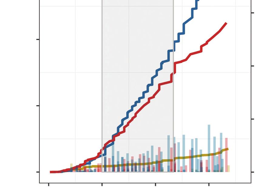
Hu et al. — Branch biomass estimation by TLS data and tree structure models                                           3

software (Leica Geosystems, 2016). Once the sample trees were                structure models. Using this method, branch biomass was esti-
extracted from the point cloud, a TreeQSM algorithm was applied              mated using a five-step process (Fig. 1) in which we:
to reconstruct the stem and branch structures. TreeQSM is a model
to reconstruct trees as hierarchical collections of cylinders and to         (1) extracted the height of each individual branch attached to
describe basic branch structure, geometric and volumetric proper-                the trunk (‘0’ branch) as observed by TreeQSM (TLS data
ties quantitatively. It has been successfully applied to derive tree             from dataset I);
volume and structure in many studies (Raumonen et al., 2013,                 (2) clustered the extracted ‘0’ branches to each whorl using a
2015; Lau et al., 2019; Raumonen, 2019; Krishna Moorthy et al.,                  criterion generated from dataset II and estimated branch
2020). Using TreeQSM, it is possible to compute various geomet-                  number at each whorl (Model 1);

                                                                                                                                                      Downloaded from https://academic.oup.com/aob/advance-article/doi/10.1093/aob/mcab037/6161336 by guest on 14 October 2021
rical stem and branch properties, such as tree height (H), diameter          (3) estimated the total branch basal area at each whorl using
at breast height (DBH), branch diameter, branch length and branch                a PMT-based tree structure model (stem taper curve and
volume.                                                                          Model 2);
                                                                             (4) estimated individual branch basal area at each whorl using
Reference measurements from destructive trees. For dataset                       tree structure models (Model 3); and
I, breast height was marked, and DBH was measured before                     (5) estimated individual branch biomass using a linear mixed
felling. For every branch originating from the trunk, we meas-                   model (Model 4).
ured the diameter and the distance from the treetop. Stem diam-
eter was measured at eight points along the stem: the stump                  Stem taper curve. We estimated the stem taper curve by mod-
point, 1.3 m, crown base, half of the crown base and 25, 50,                 elling the stem first as cylinders based on the TreeQSM method
75 and 90 % of crown length. Crown base was recorded as                      (Raumonen et al., 2013, 2015) and the results from Pitk.nen
the height of the lowest branch and a maximum of one dead                    et al. (2021). This process included three principle steps:
whorl above was allowed. A total of 811 individual branches
(including 542 living branches above the crown base and 269                  (1) co-registered TLS data were used to model the stem
dead branches) were measured. Sample branches with meas-                         roughly as a set of connected cylinders, based on their best
ured cross-diameters were selected randomly from each tenth                      fit and with no prior expectations with regard to the stem
of the crown length. A total of 60 sample branches were taken                    dimensions;
to the laboratory and dried in paper bags at 105 °C for 48 h to              (2) the cylinder model was used to split the stem into thin
determine the dry branch biomass (needles were removed from                      slices, which were further processed to refine their diam-
branches after drying).                                                          eter estimates; and
                                                                             (3) slice diameters, together with known dimensions (DBH,
Branch biomass estimation from TLS data                                          and H with a diameter of zero), were applied to construct
                                                                                 the final spline-based taper curve. This taper curve was
Overview of the TSMtls method. The TSMtls method integrated                      then used to calculate the stem diameter at any given
several models, including TLS-based and PMT-based tree                           height.

                    TLS processing                                                                    Structure models

        TLS data acquisition (Dataset I) 6 trees                              VAPU data (Dataset II) 122 trees/4797 whorls/13948 branch

                Reconstruction process
                                                                                Model 2: Bi + Bi –1 + ... B1                              Tree
                                                                                         Stem cross-sectional area at whorl i             level
       Modeling trunk and branches as cylinders

                                                                                Model 1: Branch number estimate
       Construct Stem Taper curve        Locate “0” branch’s height                                                                       Whorl
                                                                                Model 3: Individual branch diameter estimate              level

                 Total branch basal area at whorl i (Bi )                       Model 4: Individual branch biomass estimate

         Individual branch number and basal area (whorl level)                                    Branch biomass estimate

           Accuracy assessment                            Destructive measurements (Same sample trees with TLS)

                Fig. 1. Framework of TSMtls developed in this study to estimate branch biomass from TLS data and tree structure models.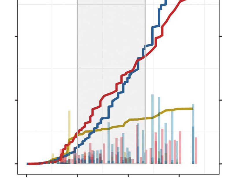
4                                  Hu et al. — Branch biomass estimation by TLS data and tree structure models

Whorl information estimation. Based on TreeQSM, the branch                                consecutive fake whorls by testing a range of values: 10–30 cm
architecture was reconstructed by segmenting the point cloud,                             with 5-cm intervals. Using each candidate interval, fake whorls
and the segments provided modelled information for each fit-                              were inserted and branch number at each whorl was estimated
ting cylinder. We selected the reconstructed branches that were                           (for details of the method see the Branch number and indi-
attached to the trunk (‘0’ branch). The branch height was then                            vidual basal area estimation section). By comparing the branch
determined and linked to the stem taper curve. Given that sev-                            number with destructive measurements, a 25-cm interval was
eral branches can be attached to one whorl, we needed to de-                              accepted in the end. Then, whorl height was calculated as the
cide whether the ‘0’ branches belonged to the same whorl. By                              average height of the ‘0’ branches in each whorl.
analysing 12 952 branches from 3802 whorls with at least two

                                                                                                                                                                       Downloaded from https://academic.oup.com/aob/advance-article/doi/10.1093/aob/mcab037/6161336 by guest on 14 October 2021
                                                                                          Branch number and individual basal area estimation. Using
branches (out of 4797 whorls in total) in 122 Scots pine trees
                                                                                          the height of each whorl as input, the stem cross-sectional
(dataset II), we found that the branches of each whorl were lo-
                                                                                          diameter at each whorl was determined using the corresponding
cated mostly within 3 cm of each other (Fig. 2C). Hence, TSMtls
                                                                                          stem taper curve. Branch number and the basal area of each in-
sets the rule thus: if the ‘0’ branch height of two consecutive                           dividual branch were then estimated using tree structure models
branches was 1 m were detected, which was not realistic. Previous                            whorl i, Nbi, was calculated as:
research has reported that the accuracy of branch extraction is                                                     b2 (H − 1.3)
highly dependent on the location of the living branch inside the                          Nbi = b0 + b1 ln (∆hi ) +
                                                                                          (1)                                   + b3 hr + εk
crown (Pyörälä et al., 2018a). Thus, for the upper crown layer,                                                         DBH
whenever the distance from the topmost whorl to the treetop was                           where b0, b1 and b2 are parameters, Δhi (cm) is the height incre-
>0.5 m, fake whorls were inserted. We optimized the interval of                           ment between whorl i and whorl i − 1, H (m) is tree height, DBH

            A                                 B                                                              D
                                                                                             A                   Dataset I
                                                                                                                    Branch height from TreeQSM

                                                  B

                                                                                                                                         A
                                                                                                                    B

                                                                                           Dataset I

                                        0.3
                                                                                                         C                                   h1
                                                          Distribution from dataset II
                                                                                                                    h2

                                        0.2
                              Density

                                        0.1

                                                                                                                    |h1-h2| ≤3 cm?
                                                                                                                    Yes: A and B from the same
                                          0                                                                         whorl;
                Dataset I                     0              20                  40                 60              No: A and B from two whorls.
                                                      Branch height discrepancy at one whorl (cm)

Fig. 2. Flowchart detailing the rules of the ‘0’ branch cluster. (A) Cloud points of a scanned sample tree. (B) Details of the branches. (C) By investigating branch
information from 4797 whorls (dataset I), the distribution of branch height discrepancy at each whorl was generated. (D) The TreeQSM algorithm can produce
cylinders of woody parts that include branch height. Example: from the TreeQSM result, the heights of branches A and B can be derived. We denote them as h1
           and h2. If |h1 − h2| ≤ 3 cm, we assume branches A and B are attached to the same whorl. Otherwise they are from two consecutive whorls.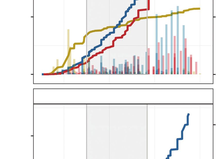
Hu et al. — Branch biomass estimation by TLS data and tree structure models                                          5

(cm) is diameter at breast height, hr is branch relative height in
                                                                                                   0.22                     0.22
the crown and εk is the random error from tree k.                  ln wbki (d) = b0 + b1 [ln(dki )] + lnεk0 + εk1 [ln(dki )] + lneki
                                                                    (6)
Model 2. Based on PMT, as presented by Makela (2002), stem
cross-sectional area Ai at the height of whorl i was proportional where b0 and b1 are fixed parameters, εk0 and εk1 are random tree
to the sum of branch basal area at and above whorl i (from parameters and eki is residual. The total branch wood biomass
whorl i to the first whorl at the top), Bi + Bi−1 + … + B1:         of each sample tree was determined by summing the biomasses
                                                                    of individual living branches.
(2)               Bi + Bi−1 + . . . + B1 = ηAi

                                                                                                                                                          Downloaded from https://academic.oup.com/aob/advance-article/doi/10.1093/aob/mcab037/6161336 by guest on 14 October 2021
where η is an empirical coefficient and Bi is the sum of branch
basal area at whorl i, calculated as follows:                                     Parameter value estimation
Bi = (Ai − Ai−1 )
(3)                                                                                 Models 1–4 have been previously tested for Scots pine in
                                                                                  south Finland (Mäkelä, 2002; Mäkinen and Mäkelä, 2003;
Model 3. Since we have the Bi and Nbi estimates, individual                       Lehtonen et al., 2004b; Hu et al., 2020). The parameter values
branch basal area distribution can be calculated using Model 3,                   of Models 1–3 applied in this study were estimated based on
taken from Mäkinen and Mäkelä (2003). Firstly, the relative                       dataset II. The parameter values for eqn (6) (Model 4) have
sizes of the largest (Ri max) and smallest (Ri min) living branches               been estimated previously using the same VAPU dataset
in whorl i were defined as Model 3: the largest and smallest                      (Lehtonen et al., 2004b). For mixed effect models [eqns (1),
branch basal area in whorl i divided by the mean branch basal                     (4)–(6)], parameters were estimated using the lmer function in
area in whorl i. The models for Ri max and Ri min were estimated                  R from the lme4 package (Bates et al., 2014) and pseudo-R2
using the following equations:                                                    was calculated using the r.squaredGLMM function in R from
                                                                                  the MuMIn package as an evaluation indicator (Nakagawa and
lnRi    max   = b0 + b1 Nbi + b2 (1.1 − hri )                                     Schielzeth, 2013).
(4)    + b3 ln (1.1 − hri ) + b4 DBH + b5 H/DBH + εk
   Å            ã
       Ri min                                                                     Model evaluation
ln                = b0 + b1 Nbi + b2 (1.1 − hri )
     1 − Ri min
                                                                                     We used sample trees from dataset I to compare the ac-
(5)                 + b3 ln (1.1 − hri ) + b4 DBH + εk                           curacy of whorl and branch estimates from the TSMtls method
                                                                                  (against reference measurements) with the accuracy obtained
where b0–5 are parameters, Ri is the relative size of the branch in               directly from a TreeQSM algorithm (against reference meas-
whorl i, Nbi is the number of branches in whorl i, hri is the branch              urements). The comparison combined: (1) a tree-level variable,
relative height in the crown (distance from the tree top to whorl                 i.e. the number of whorls; and (2) whorl-level variables, which
i divided by crown length) and εk is the random error from tree                   included branch number, diameter and biomass (Table 2). To
k. Then, individual branch size was drawn from a uniform dis-                     evaluate tree- and whorl-level results, we manually paired in-
tribution and Ri max and Ri min were used as the constraints. For the             dividual whorls from the TSMtls method and destructive meas-
whorls that were estimated as having only one branch, branch                      urement. To locate each whorl, we paired each measured whorl
basal area was assumed to be Bi. Thus, individual branch diameter                 with the modelled one that was the closest to the measurement
can be derived according to branch basal area.                                    with respect to stem cross-sectional area. Since we inserted the
Model 4. Finally, individual branch biomass was estimated                         fake whorls in the top of the crown, we examined the perform-
using a mixed linear model as in Lehtonen et al. (2004b) and                      ance of the TSMtls method separately at the upper, middle and
the whole-tree branch wood biomass was the sum of indi-                           lower crown. We classified the living branches inside the crown
vidual branch biomass. Let wbki be the dry weight of branch                       into three layers on the basis of relative height in the crown:
i on tree k, then wbki can be modelled as a function of branch                    (1) upper crown
6                               Hu et al. — Branch biomass estimation by TLS data and tree structure models

and omission error (Eo) of whorl/branch number were defined
for each crown layer as well as for the whole tree using the fol-                           n                      2
                                                                                (10)        1 (Wb model − Wb ref )
lowing equations:                                                               RMSE (kg) =
                                                                                                      n
                      Np
Accuracy ( % ) =
(7)                          × 100                                                              RMSE
                 Np + Nc + No                                                   CV RMSE ( % ) = n           × 100
                                                                                (11)
                                                                                                 1 Wb ref /n
                Nc
Ec ( % ) =
(8)                    × 100
           Np + Nc + No

                                                                                                                                                   Downloaded from https://academic.oup.com/aob/advance-article/doi/10.1093/aob/mcab037/6161336 by guest on 14 October 2021
                                                                                                                RESULTS
                No
Eo ( % ) =
(9)                    × 100
           Np + Nc + No                                                         Model parameter values
where Np is the number of paired whorls/branches, Nc is the                     In this study, parameters of Models 1–4 were estimated based
number of commission errors, i.e. the number of whorls/                         on dataset II (Table 4). For linear mixed models [eqns (1), (4)–
branches that were falsely detected or modelled, and No is the                  (6)], only the fixed part was applied to the TSMtls method for
number of omission errors, i.e. the number of whorls/branches                   estimating branch number, diameter and biomass.
omitted from the measurements. Moreover, the correspondence
between measured and estimated individual branch diameter
was evaluated by comparing the whorl mean, whorl maximum
and whorl minimum diameters with destructive measurements.                      Whorl number evaluation
The two-sample Kolmogorov–Smirnov (KS) test and com-                              Whorl number was estimated for sample trees in dataset
parisons of the cumulative distribution function were used to                   I using three approaches (Table 2). The TSMtls method im-
analyse whether the individual branch biomass distributions in                  proved whorl number estimate accuracy from 40.43 to 57.73 %
three crown layers determined by TreeQSM and TSMtls were                        compared with the TreeQSM method, and the upper crown
different from our destructive measurements.                                    showed the highest improvement of accuracy, from 29.20 to
                                                                                52.59 % (Table 5, Fig. 3). In addition, commission error (Ec)
                                                                                and omission error (Eo) were reduced by 14.38 and 3.01 per-
                                                                                centage points, respectively (Fig. 3A–C, Table 5).
Total branch biomass from other TLS-based models
   Additionally, we tested the performance of our total branch
biomass estimates against tree-level allometric models evalu-                   Branch information evaluation
ated with TLS-based input variables. Here we used empirical
allometric (denoted QSM_Allometry) (Repola, 2009) and pipe-                     Branch number (Model 1). With the TSMtls method, branch
model based equations (denoted QSM_CROBAS) (Valentine                           number was estimated for each individual whorl. For the 199
and Mäkelä, 2005; Hu et al., 2020). These two methods util-                     paired whorls, the TSMtls method had an overall accuracy of
ized the tree height and diameter derived from TreeQSM as                       68.60 % and registered its highest improvement (from 28.94
inputs with parameter values as presented in previous literature                to 68.92 %) compared with the TreeQSM method in the upper
(Table 3). We used linear regression to compare the different                   layer of the crown (Table 6). Using the TSMtls method, Ec and
approaches with reference to destructive measurements. As                       Eo relative to the destructively measured branches were 22.24
general indicators of the accuracy of the model approaches,                     and 9.16 %, respectively. The inserted fake whorls in the upper
R2, root mean square error (RMSE) [eqn (10)] and the coeffi-                    crown led to more commission errors (42 more cases) than
cient of variation (CV) of the RMSE [eqn (11)] of total branch                  TreeQSM, but the respective omission error decreased almost
biomass estimation were calculated. In addition, we also used                   6-fold (97 fewer cases) (Table 6).
the concordance correlation coefficient (CCC) (Lawrence and                     Branch diameter and biomass (Models 2, 3 and 4). Within
Lin, 1989) to compare agreement of model estimates with                         paired whorls, the diameter estimation of the largest branch
reference.                                                                      had a lower relative error (31.2 %) than the smallest branch

Table 3. Model description for the TLS-derived branch woody biomass estimations, including stump diameter (dS, m), wood density (ρb,
kg m−3), height (H, m), stem cross-sectional area at crown base (Ac, m2), and parameters used in each equation. QSM_Allometry was
                                   based on Repola (2009) and QSM_CROBAS on Hu et al. (2020)

Models                     Equations                                   ρb            a               b                c          φb       ηs/ηb

TreeQSM                    Wb = Vcylinder × ρb                         400           –               –                –          –        –
QSM_Allometry              In(Wb ) = a + b × dsd+6
                                                s
                                                   +c×    H            –             –6.16           15.08            –2.62      –        –
                                                         H+1
QSM_CROBAS                 Wb = ρb × ϕb × ηs /ηb × Ac                  400           –               –                –          1.16     1.65

TSMtls*                    Wb = i1 Wbj                                 –             –               –                –          –        –

    *Total branch biomass from TSMtls was calculated by summing individual branch biomass (wbj, kg) based on Model 4, eqn (6).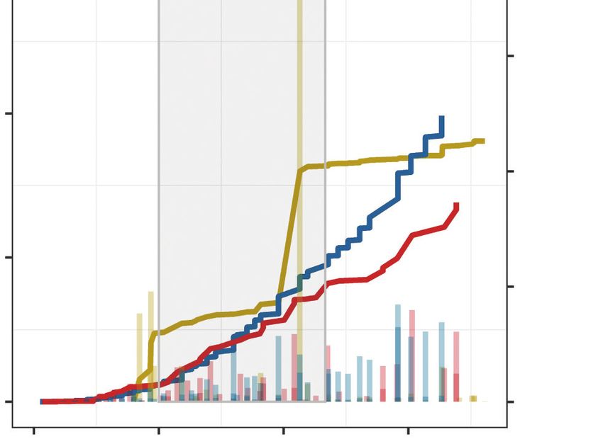
Table 4. Parameter estimate and CV of each parameter in Models 1–4. Numbers in parentheses were the modelling sample numbers from dataset II used to estimate the
                                                                        parameters

Parameter             Eqn (1) (4797)                         Eqns (2) and (3) (4797)                  Eqn (4) (4797)                         Eqn (5) (4797)                          Eqn (6) (13 984)* 1

                      Estimate             CV                Estimate              CV                 Estimate             CV                Estimate              CV                Estimate              CV

Fixed part
  η                 –                                        1.810                 0.002              –                                      –                                       –
  b0                1.514                  0.197             –                     –                  0.237                0.249             0.894                 0.210             –36.100               0.011
  b1                0.883                  0.041             –                     –                  0.079                0.063             –0.412                0.058             32.514                0.010
  b2                –0.712                 0.567             –                     –                  –0.277               0.097             1.404                 0.106             –                     –
  b3                –0.405                 0.163             –                     –                  0.036                0.194             –0.214                0.187             –                     –
  b4                –                      –                 –                     –                  0.001                0.000             –0.004                0.000             –                     –
  b5                –                      –                 –                     –                  –0.007               0.571             –                     –                 –                     –
Random part
  εk (εk0 )
            ∗2
                    0.578                  0.019             –                     –                  0.005                0.254             0.060                 0.072             0.048                 0.002
  εk1               –                      –                 –                     –                  –                    –                 –                     –                 5.846                 0.005
Residual            1.109                  0.014             –                     –                  0.043                0.086             0.989                 0.018             0.182                 0.001
Whole-model evaluation
   R2m * 3          0.246                  –                 0.980                 –                  0.457                –                 0.223                 –                 0.890                 –
   R2c              0.421                  –                 –                     –                  0.554                –                 0.256                 –                 0.910                 –
  RMSE              1.097                  –                 0.003                 –                  0.219                –                 1.023                 –                 1.814                 –

   * 1Parameters were estimated by Lehtonen et al. (2004b) using the same dataset; *2εk0 and εk1 were only applied to eqn (6); * 3 R2m is the marginal r2 value representing the variance explained by the fixed
effects; R2c is the conditional r2 value representing the variance explained by the entire model, including both fixed and random effects.
                                                                                                                                                                                                                   Hu et al. — Branch biomass estimation by TLS data and tree structure models
                                                                                                                                                                                                                   7

                                 Downloaded from https://academic.oup.com/aob/advance-article/doi/10.1093/aob/mcab037/6161336 by guest on 14 October 2021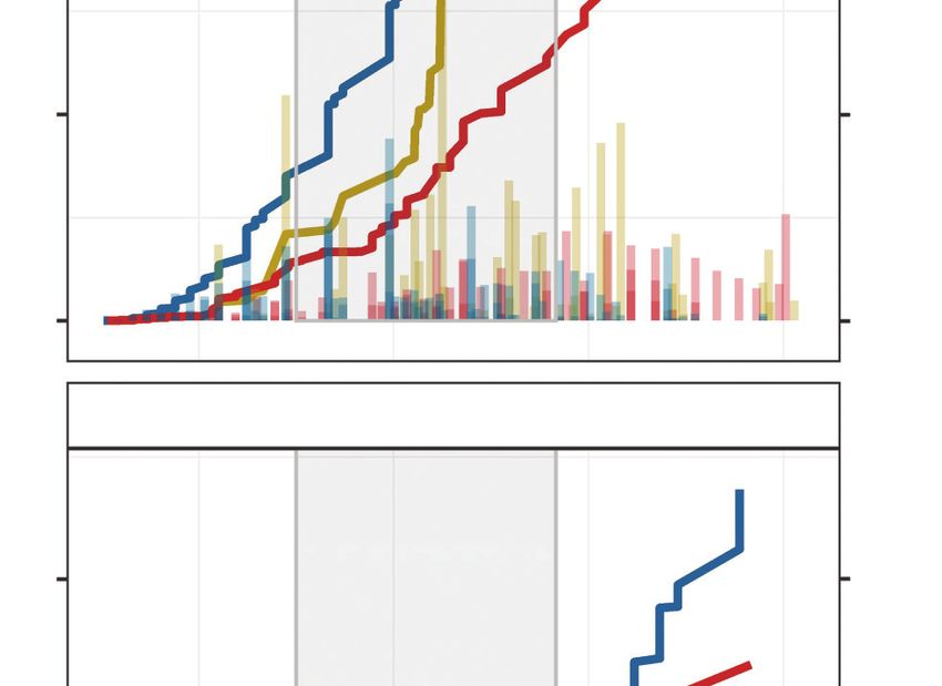
8

Table 5. Paired whorl number (Np), commission number (Nc) and omission number (No) between estimated whorl number and reference destructive measurement at different
      crown layers and whorl tree levels, with TEMtls and TreeQSM methods. Whorl number accuracy, commission error (Ec) and omission error (Eo) are also listed

Tree no.   Crown layer   Ref.     TreeQSM                                                                TSMtls

                                  Total     Np     Nc      No      Accuracy (%)     Ec (%)    Eo (%)     Total    Np      Nc     No     Accuracy (%)   Ec (%)   Eo (%)

11         Total          32       20        15      5      17     40.54           13.89       44.44      29       26      3      6     74.29           8.57    17.14
           Upper           9        0         0      0       9      0.00            0.00      100.00      11        9      2      0     81.82          18.18     0.00
           Middle         12       12        10      2       2     71.43           14.29       14.29      11       10      1      2     76.92           7.69    15.38
           Lower          11        8         5      3       6     35.71           21.43       42.86       7        7      0      4     63.64           0.00    36.36
12         Total          41       55        29     26      12     43.28           38.81       17.91      46       32     14      9     58.18          25.45    16.36
           Upper          13        5         5      0       8     38.46            0.00       61.54       9        9      0      4     69.23           0.00    30.77
           Middle         16       30        16     14       0     53.33           46.67        0.00      22       16      6      0     72.73          27.27     0.00
           Lower          12       20         8     12       4     33.33           50.00       16.67      15        7      8      5     35.00          40.00    25.00
31         Total          49       78        37     41      12     41.11           45.56       13.33      53       36     17     13     54.55          25.76    19.70
           Upper          23       16        12      4      11     44.44           14.81       40.74      15       13      2     10     52.00           8.00    40.00
           Middle         16       41        16     25       0     39.02           60.98        0.00      25       14     11      2     51.85          40.74     7.41
           Lower          10       21         9     12       1     40.91           54.55        4.55      13        9      4      1     64.29          28.57     7.14
32         Total          41       45        27     18      14     45.76           30.51       23.73      46       33     13      8     61.11          24.07    14.81
           Upper          18        5         4      1      14     21.05            5.26       73.68      17       12      5      6     52.17          21.74    26.09
           Middle         15       17        15      2       0     88.24           11.76        0.00      16       13      3      2     72.22          16.67    11.11
           Lower           8       23         8     15       0     34.78           65.22        0.00      13        8      5      0     61.54          38.46     0.00
41         Total          55       51        31     20      24     41.33           26.67       32.00      43       37      6     18     60.66           9.84    29.51
           Upper          29       14         9      5      20     26.47           14.71       58.82      15       14      1     15     46.67           3.33    50.00
           Middle         16       28        15     13       1     51.72           44.83        3.45      20       15      5      1     71.43          23.81     4.76
           Lower          10        9         7      2       3     58.33           16.67       25.00       8        8      0      2     80.00           0.00    20.00
42         Total          54       67        30     37      24     32.97           40.66       26.37      52       34     18     20     47.22          25.00    27.78
           Upper          31       14        10      4      21     28.57           11.43       60.00      16       14      2     17     42.42           6.06    51.52
           Middle         14       29        13     16       1     43.33           53.33        3.33      19       13      6      1     65.00          30.00     5.00
           Lower           9       24         7     17       2     26.92           65.38        7.69      17        7     10      2     36.84          52.63    10.53
Total      All           272      316       169    147     103     40.33           35.17       24.40     269      198     71     74     57.73          20.70    21.57
                                                                                                                                                                         Hu et al. — Branch biomass estimation by TLS data and tree structure models

                          Downloaded from https://academic.oup.com/aob/advance-article/doi/10.1093/aob/mcab037/6161336 by guest on 14 October 2021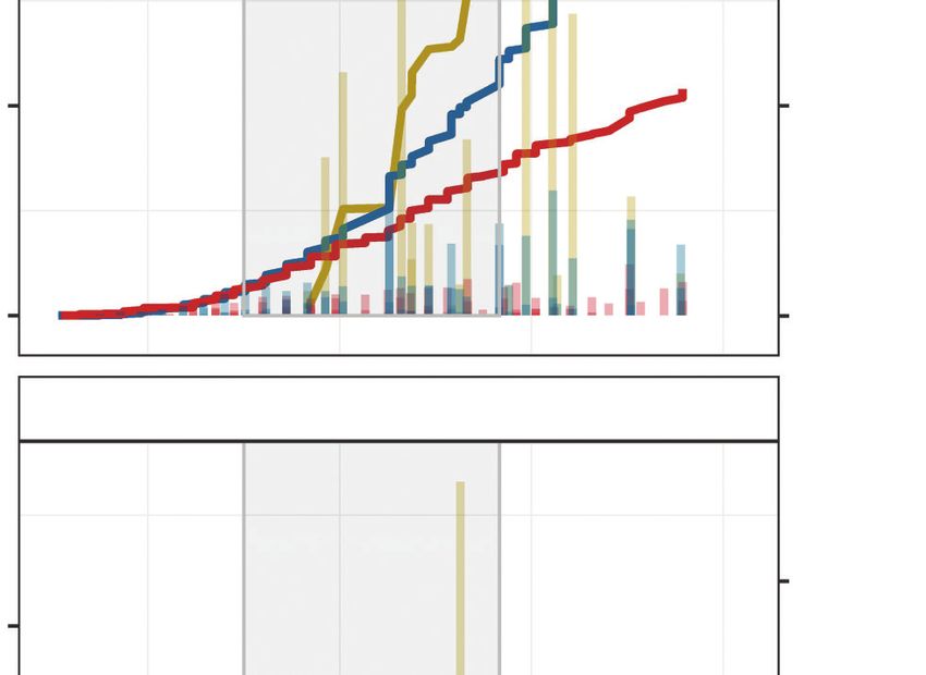
Hu et al. — Branch biomass estimation by TLS data and tree structure models                                       9

                                                                                                                                                   TreeQSM         TSMtls

                                                  Whorl number accuracy                       Whorl number Ec                            Whorl number Eo
                                100   A                                           B                                          C
                                             aT           aL   aM aM         aU                                                                               aU
                                                                                              aL    aL
                                                     bL
                                 75
                                                                                                         aM aM                                                      bU
                                      bT                                bU        aT                                         aT aT       aL   aL

                                                                                                                                                                                Downloaded from https://academic.oup.com/aob/advance-article/doi/10.1093/aob/mcab037/6161336 by guest on 14 October 2021
                                 50
                                                                                         aT
                                                                                                                   aU aU                            aM aM

                                 25
     Evaluation indicator (%)

                                  0

                                                  Branch number accuracy                      Branch number Ec                           Branch number Eo
                                                                                                                                                              aU
                                100   D                                           E                                          F
                                                                             aU
                                                     aL aL     aM aM
                                            aT                                                                               aT

                                      bT                                                                                                            aM
                                 75
                                                                                                                                         aL aL

                                                                                              aL    aL        aM
                                 50
                                                                                                                                                                    bU
                                                                                         aT                             aU          bT                   bM
                                                                                                         bM
                                                                                   bT                              bU
                                 25

                                  0

                                          Total      Lower     Middle     Upper       Total    Lower      Middle   Upper         Total    Lower     Middle    Upper
                                                                                                   Crown layer

Fig. 3. Box plots showing accuracy, commission error (Ec) and omission error (Eo) for whorl (A, B, C) and branch number (D, E, F) estimates in the whole tree
and in different crown layers using TreeQSM and TSMtls approaches. Box dimensions show the quartiles for 25–75 % accuracy, the black line represents median
indicator values and the whiskers show minimum and maximum values. Lower-case letters a, b on the boxplots show the significance of each indicator between
                        different approaches (P < 0.05) and subscripts T, L, M and U represent the whole tree and different crown layers.

estimation (52.6 %) (Fig. 4). Nevertheless, both models                                               measurements in all the crown layers of each sample (Fig. 5).
[eqns (5) and (6)] underestimated the branch diameter, and                                            It indicated a significant improvement of the individual branch
the underestimation was more pronounced on the smallest                                               biomass estimate using the TSMtls method. For the TreeQSM
individual in each whorl, with a proportion of 73.8 % of the                                          method, some extreme individual branch biomass estimates
smallest branches being underestimated. Furthermore, the                                              (Fig. 6) and unobserved branches (Fig. 3C, tree 11) could be
empirical cumulative distribution function (ECDF) of indi-                                            the main reasons behind the bias of the total branch biomass
vidual branch biomass from the TSMtls method showed that                                              (Table 7).
the bias occurred more in the middle and lower part of the
crown (Fig. 5, P < 0.05).
  Although branch diameters were underestimated, the cu-                                              Total branch biomass from TLS-based models. When com-
mulative branch biomass estimated by the TSMtls method                                                pared with destructive branch biomass measurements, the
agreed much better with the destructive measurements than                                             TSMtls method showed 1.76 and 25.27 kg lower RMSE and
the TreeQSM method (Fig. 6, Table 7) at the tree level.                                               3.31 and 47.79 percentage points lower CV RMSE than the
Moreover, the KS test showed that individual branch estimates                                         QSM_CROBAS and TreeQSM methods. The performance of
produced by the TSMtls method had lower D statistic values                                            the QSM_Allometry method was intermediate between the
than the TreeQSM method when compared with destructive                                                QSM_CROBAS and TreeQSM methods. The TSMtls method
10

Table 6. Paired branch number (Np), commission number (Nc) and omission number (No) between estimated whorl number and reference destructive measurement at dif-
  ferent crown layers and whorl tree levels, with TSMtls and TreeQSM approaches. Whorl number accuracy, commission error (Ec) and omission error (Eo) are also listed

Tree no.   Crown Layer    Ref.    TreeQSM                                                               TSMtls

                                  Total     Np     Nc     No      Accuracy (%)     Ec (%)    Eo (%)     Total    Np      Nc      No     Accuracy (%)   Ec (%)   Eo (%)

11         Total           87      19        18     1      69     20.45             1.14      78.41      69       65       4     22     71.43           4.40    24.18
           Up              37       0         0     0      37      0.00             0.00     100.00      28       28       0      9     75.68           0.00    24.32
           Middle          34      11        11     0      23     32.35             0.00      67.65      27       25       2      9     69.44           5.56    25.00
           Lower           16       8         7     1       9     41.18             5.88      52.94      14       12       2      4     66.67          11.11    22.22
12         Total           81      38        37     1      44     45.12             1.22      53.66      86       69      17     12     70.41          17.35    12.24
           Up              29       5         5     0      24     17.24             0.00      82.76      28       24       4      5     72.73          12.12    15.15
           Middle          35      20        20     0      15     57.14             0.00      42.86      37       30       7      5     71.43          16.67    11.90
           Lower           17      13        12     1       5     66.67             5.56      27.78      21       15       6      2     65.22          26.09     8.70
31         Total           70      59        49    10      21     61.25            12.50      26.25      79       61      18      7     70.93          20.93     8.14
           Up              18      13        11     2       7     55.00            10.00      35.00      24       18       6      0     75.00          25.00     0.00
           Middle          34      29        24     5      10     61.54            12.82      25.64      40       31       9      1     75.61          21.95     2.44
           Lower           18      17        14     3       4     66.67            14.29      19.05      15       12       3      6     57.14          14.29    28.57
32         Total           50      42        32    10      18     53.33            16.67      30.00      74       48      26      2     63.16          34.21     2.63
           Up              20       5         5     0      15     25.00             0.00      75.00      26       18       8      2     64.29          28.57     7.14
           Middle          16      16        14     2       2     77.78            11.11      11.11      25       16       9      0     64.00          36.00     0.00
           Lower           14      21        13     8       1     59.09            36.36       4.55      23       14       9      0     60.87          39.13     0.00
41         Total           63      45        39     6      24     56.52             8.70      34.78      91       63      28      0     69.23          30.77     0.00
           Up              27      13        11     2      16     37.93             6.90      55.17      41       27      14      0     65.85          34.15     0.00
           Middle          28      23        21     2       7     70.00             6.67      23.33      35       28       7      0     80.00          20.00     0.00
           Lower            8       9         7     2       1     70.00            20.00      10.00      15        8       7      0     53.33          46.67     0.00
42         Total           67      46        43     3      23     62.32             4.35      33.33      87       61      26      6     65.59          27.96     6.45
           Up              25      11        10     1      15     38.46             3.85      57.69      39       24      15      1     60.00          37.50     2.50
           Middle          28      23        22     1       5     78.57             3.57      17.86      32       26       6      2     76.47          17.65     5.88
           Lower           14      12        11     1       3     73.33             6.67      20.00      16       11       5      3     57.89          26.32    15.79
Total      All            418     249       218    31     199     48.66             6.92      44.42     486      367     119     49     68.60          22.24     9.16
                                                                                                                                                                         Hu et al. — Branch biomass estimation by TLS data and tree structure models

                          Downloaded from https://academic.oup.com/aob/advance-article/doi/10.1093/aob/mcab037/6161336 by guest on 14 October 2021
Hu et al. — Branch biomass estimation by TLS data and tree structure models 11
Largest
y = 0.69x + 11.52 R 2 = 0.51
90
Estimated branch diameter at each whorl (mm)
RMSE = 12.79 (mm)
Relative error = 31.2%
Downloaded from https://academic.oup.com/aob/advance-article/doi/10.1093/aob/mcab037/6161336 by guest on 14 October 2021
Mean
60 y = 0.48x + 10.23 R 2 = 0.50
RMSE = 8.62 (mm)
Relative error = 37.8%
Smallest
30
y = 0.21x + 8.25 R 2 = 0.38
RMSE = 4.78 (mm)
Relative error = 52.6%
0
0 25 50 75
Measured branch diameter at each whorl (mm)
Fig. 4. Comparison of destructive measurement- and TSMtls-based individual branch diameter (n = 594). Large, small and medium dots denote whorl maximum,
minimum and mean diameter, respectively.
was closer to the 1:1 line and the agreement between TSMtls features (time-of-flight scanner): the signal will return as soon
estimates and destructive measurements expressed as CCC was as it reaches a non-penetrable obstacle, rendering the cloud
higher (0.99) than those of the other TLS-based models (0.43– points unavailable for locations not visible from the scanner.
0.98; Table 7). As the lower branches may hinder visibility, fewer signals will
reach the upper branches, which may cause branch omission.
Moreover, the upper canopy is further from the scanner, which
DISCUSSION makes the point cloud naturally sparser compared with the
lower parts.
This study proposes a method to estimate branch biomass In addition, in TreeQSM results it is not hard to notice the ab-
by linking TLS data with tree structure models. The re- normal outliers that feature extremely large individual branch
sults showed that the TSMtls method of estimating total biomass (Fig. 6). This is because the main task of TreeQSM is
branch biomass is more accurate than the other TLS-based to reconstruct the woody part as cylinders (Raumonen et al.,
approaches tested. 2013). To get an accurate result, this procedure needs enough
points, and fewer points increase the likelihood of misevaluated
branch diameters. Weather effects such as wind can result in
Individual branch extraction from TLS noisy data while scanning and detract from the ability to re-
construct individual branch structures. Additionally, our sample
The TreeQSM method has been widely used in tree struc- trees are Scots pine, which have needles all year round, and this
ture or biomass estimation (Gonzalez De Tanago et al., 2017; makes it harder to get the leaf-off scanned data.
Lau et al., 2018, 2019). Our main rationale for developing the
method further was its inaccurate individual branch extraction.
Even though several scans were taken from different points
TSMtls method considerations
around the target trees to gain more comprehensive branch in-
formation, many of the branches were still not observed, es- The TSMtls method relies on the PMT-based equation, in
pecially in the upper part of the crown, which showed higher which the stem cross-sectional basal area and branch basal
omission error than the lower part (Figs 3C and 6). This has area at each whorl are linearly related [eqn (2)], which has
been observed in previous studies as well (Eysn et al., 2013; been demonstrated in previous studies (Makela, 2002; Kantola
Boudon et al., 2014) and it was mainly caused by the scanner’s and Mäkelä, 2004, 2006). This linear relationship was used12 Hu et al. — Branch biomass estimation by TLS data and tree structure models
TreeQSM TSMtls Measurement
11 12 21 22 31 32
1.00
0.75
Upper
0.50
TreeQSM TreeQSM TreeQSM TreeQSM TreeQSM TreeQSM
na 0.676 * 0.539 *** 0.800 *** 0.633 *** 0.309 ns
Downloaded from https://academic.oup.com/aob/advance-article/doi/10.1093/aob/mcab037/6161336 by guest on 14 October 2021
0.25
TSMtls TSMtls TSMtls TSMtls TSMtls TSMtls
0.169 ns 0.246 ns 0.197 ns 0.286 ns 0.251 ns 0.194 ns
0
1.00
Cumulative probability
0.75
Middle
0.50
TreeQSM TreeQSM TreeQSM TreeQSM TreeQSM TreeQSM
0.644 *** 0.315 ns 0.197 *** 0.495 ** 0.750 *** 0.935 ***
0.25
TSMtls TSMtls TSMtls TSMtls TSMtls TSMtls
0.315 * 0.161 ns 0.354 ns 0.412 ** 0.495 *** 0.428 ***
0
1.00
0.75
Lower
0.50
TreeQSM TreeQSM TreeQSM TreeQSM TreeQSM TreeQSM
0.739 *** 0.400 ns 0.904 *** 0.857 *** 0.833 *** 0.850 ***
0.25
TSMtls TSMtls TSMtls TSMtls TSMtls TSMtls
0.470 * 0.750 *** 0.388 ns 0.400 ns 0.400 *** 0.378 ns
0
0 5000 10 000 0 5000 10 000 0 5000 10 000 0 5000 10 000 0 5000 10 000 0 5000 10 000
Individual branch biomass (g)
Fig. 5. Comparison of the empirical cumulative distribution of individual branch biomass among TreeQSM, TSMtls and measurements presented by different
crown layers in the six test trees (tree ID number is in the box at the top of each panel). Values in the figure are the D statistic values from the KS test, which quan-
tify the maximum vertical distances between TreeQSM/TSMtls-based distribution and measurement distribution. Asterisks denotes the significance level in the KS
test: ns, not significant; *P < 0.05; **P < 0.01; ***P < 0.001. In the upper crown of tree 11 no branches were extracted from TreeQSM, and therefore the KS test
was not applied to TreeQSM (marked as na).
in Model 2, and, together with Model 1, individual branches age influenced the accuracy of the model. Additionally, branch
were simulated in each whorl. It is not surprising that the growth is also affected by shading or interaction with other
total branch biomass estimates were in closer agreement with branches and trees, especially for the branches in the middle or
destructive measurements using TSMtls than the TreeQSM lower part of the crown. This could result in fewer branches in
method (Table 7), because many branches failed to be ob- reality than modelled and is also consistent with our result that
served when using the TreeQSM method (Fig. 3). Also, in the the modelled individual branch biomass distribution had more
TSMtls method we optimized the interval value of consecutive bias in the lower than the upper crown (Fig. 5). Hence, the over-
fake whorls based on destructive measurements, which could estimated branch number leads to a smaller mean branch basal
also contribute to better results compared with the TreeQSM area for a given whorl total, which may be one reason why the
method. This means that an optimized interval value of con- branch basal area was underestimated (Fig. 4). Nevertheless,
secutive whorls may need to be considered properly when the accuracy of the branch number estimate (68.60 %) was im-
TSMtls is applied to another dataset. Nevertheless, the indi- proved compared with previous studies: Pyörälä et al. (2018a)
vidual branch number and diameter estimates were still biased extracted individual Scots pine branches with an accuracy of
using TSMtls (Figs 3 and 4). One reason could be that the 64.8 % and Pyörälä et al. (2018b) reported a higher branch
branch number model we used was developed on the basis of number detection accuracy (69.9 %), but they only considered
branch data from trees in the age range of 22–76 years (Mäkelä the largest branches of whorls, where stem diameter exceeded
and Mäkinen, 2003), while the age range of the trees sampled 15 cm. Other studies focusing on individual branch informa-
(dataset I) was 91–113 years and dataset II comprised trees tion also indicate that the larger the branch, the easier it is to
of various ages in our study. In eqn (1), annual height growth detect, even if only relatively large branches are considered
and slenderness were considered the main variables reported (Lau et al., 2018).
to be affected by tree age (Hann and Larsen, 1991; Helmisaari The present TSMtls approach has been motivated by the con-
et al., 2002; Weiskittel et al., 2011), and it is possible that the venience of TLS and the idea of PMT-based carbon allocationHu et al. — Branch biomass estimation by TLS data and tree structure models 13
TreeQSM TSMtls Measurement
11 12 21
40 10.0
40 10.0
60 15
30 7.5 30 7.5
40 10
20 5.0 20 5.0
Downloaded from https://academic.oup.com/aob/advance-article/doi/10.1093/aob/mcab037/6161336 by guest on 14 October 2021
Cumulative branch biomass (kg)
20 5
Individul branch biomass (kg)
10 2.5 10 2.5
0 0 0 0 0 0
22 31 32
40
20 60 15 150
75
30
15
40 10 100
50
20
10
25 20 5 50
5 10
0 0 0 0 0 0
0 0.3 0.6 0.9 0 0.3 0.6 0.9 0 0.3 0.6 0.9
Relative distance to the tree top
Fig. 6. Comparison of cumulative (lines, primary y-axis) and individual branch (histograms, secondary y-axis) biomass estimates from TreeQSM, TSMtls and
destructive measurements at relative height of each sample tree (tree ID number is in the box at the top of each panel). The grey area shows the middle part of the
crown.
Table 7. Summary of total branch biomass estimates from TLS-based models. For R2, RMSE, CV RMSE and CCC, n = 6. Slope and
intercept values come from the regression models between TLS-based models and measurements. Models are arranged according to
performance from the worst to the best
Model Slope Intercept R2 RMSE (kg) CV RMSE ( %) CCC
TreeQSM −2.46 112.2 0.27 30.37 57.45 0.43
QSM_Allometry 2.26 −11.90 0.91 10.58 20.02 0.95
QSM_CROBAS 0.69 1.79 0.96 6.86 12.97 0.98
TSMtls 0.72 5.08 0.98 5.10 9.66 0.99
(Mäkelä and Mäkinen, 2003; Mäkinen and Mäkelä, 2003). This and biomass in the paired whorls, the total branch biomass
method allows branch biomass estimation without destructively estimates obtained using the TSMtls method showed close
harvesting the trees. The results are encouraging; however, only agreement with the measured trees (Fig. 6) and this method
a limited dataset was used for validation. In order to apply this performed better than the other TLS-based methods (Table
method in operational work, a larger dataset would be required 7). This is in line with the result that the estimate of total
to confirm our results in the future. basal area of branches at each whorl (Model 2) was unbiased,
as predicted by the PMT (Shinozaki et al., 1964b), and sug-
gests that it is more accurate for total biomass estimation
than individual branch attributes.
Tree-level branch biomass estimation by different methods In contrast, traditional allometry models for estimating total
branch biomass are based on breast height or stump diameter and
At the whole-tree level, four different TLS-based methods
tree height (Kärkkäinen, 2005; Repola et al., 2007). Although
to predict the total branch biomass were compared. Despite
these models have been applied to different species and sites, and
the notable underestimation of individual branch diameter14 Hu et al. — Branch biomass estimation by TLS data and tree structure models
the variables used in the models are easy to measure and extract IBC-CARBON (grant 2017/312559) and the Biogeochemical
from TLS data, the reliability and applicability of the estimates and biophysical feedbacks from forest harvesting to climate
still depend on data from different studies (Repola, 2009). Parresol change project (grant 325680) from the Academy of Finland.
(1999) found that the total branch biomass varies from stand to
stand even with the same tree height and trunk diameter due to
different growth conditions, reducing the precision of the biomass ACKNOWLEDGEMENTS
estimate using allometry models. Though Repola (2008) has de-
We thank Che Liu, Kourosh K. Koupaei, Atte T. Kumpu and
veloped multivariate mixed models to estimate tree component
Jian Liu for the field work in Lapinjärvi in 2018. We appreciate
biomass better by considering simultaneous correlation between
Downloaded from https://academic.oup.com/aob/advance-article/doi/10.1093/aob/mcab037/6161336 by guest on 14 October 2021
the work by the field teams from the Finnish Forest Research
different tree components (foliage, branch, stem and root), it is still
Institute (METLA) for collecting VAPU data.
a challenge to use TLS data alone to obtain biomass estimation
models for each tree component. From this perspective, it is not
surprising that a PMT-based model together with TLS data could
provide a more reliable and accurate branch biomass estimate than
allometry models. LITERATURE CITED
Atkins JW, Bohrer G, Fahey RT, et al. 2018. Quantifying vegetation
and canopy structural complexity from terrestrial LiDAR data using
the FORESTR R package. Methods in Ecology and Evolution 9:
Potential application of TSMtls 2057–2066.
Bates D, Mächler M, Bolker B, Walker S. 2014. Fitting linear mixed-effects
This study proposes a new method to estimate branch biomass models using lme4. arXiv preprint arXiv:1406.5823.
based on TLS data with tree structure models, which provides a Boudon F, Preuksakarn C, Ferraro P, et al. 2014. Quantitative assessment of
automatic reconstructions of branching systems obtained from laser scan-
non-destructive means of investigating the vertical branch dis- ning. Annals of Botany 114: 853–862.
tribution in the crown. Firstly, as the basis of branch attribute Delucia EH, Maherali H, Carey EV. 2000. Climate-driven changes in bio-
estimation, PMT-based tree structure models have been tested mass allocation in pines. Global Change Biology 6: 587–593.
for Norway spruce and silver birch in previous studies (Ilomäki Eysn L, Pfeifer N, Ressl C, et al. 2013. A practical approach for extracting
et al., 2003; Kantola and Mäkelä, 2004; Kantola and Mäkelä, tree models in forest environments based on equirectangular projections
of terrestrial laser scans. Remote Sensing 5: 5424–5448.
2006; Hu et al., 2020). This suggests that we could apply our Gonzalez De Tanago J, Lau A, Bartholomeus H, et al. 2017. Estimation
method to more species, such as Norway spruce, which require of above-ground biomass of large tropical trees with terrestrial LiDAR.
greater effort in field measurements due to their dense foliage. Methods in Ecology and Evolution 9: 223–234.
Secondly, recent advances in TLS data processing have en- Hann DW, Larsen DR. 1991. Diameter Growth Equations for Fourteen Tree
Species in Southwest Oregon. For. Res. Lab., Oregon State University
abled us to produce relatively accurate and unbiased stem taper Research Bulletin 69, 18.
curves in boreal forests (Pitkänen et al., 2019, 2021), which Hauglin M, Astrup R, Gobakken T, Næsset E. 2013. Estimating single-tree
further contributes to the estimation of branch basal areas of branch biomass of Norway spruce with terrestrial laser scanning using
each whorl. Although our scanned sample trees (dataset I) are voxel-based and crown dimension features. Scandinavian Journal of
limited in number and focused on Scots pine only, TSMtls still Forest Research 28: 456–469.
Helmisaari H-S, Makkonen K, Kellomäki S, Valtonen E, Mälkönen E.
has potential and value in measuring more species and over a 2002. Below- and above-ground biomass, production and nitrogen use
larger area. in Scots pine stands in eastern Finland. Forest Ecology and Management
165: 317–326.
Hu M, Lehtonen A, Minunno F, Mäkelä A. 2020. Age effect on tree struc-
ture and biomass allocation in Scots pine (Pinus sylvestris L.) and Norway
Conclusions spruce (Picea abies [L.] Karst.). Annals of Forest Science 77: 1–15.
Ilomäki S, Nikinmaa E, Mäkelä A. 2003. Crown rise due to competition
In this study we present a new method that not only estimates drives biomass allocation in silver birch. Canadian Journal of Forest
branch biomass precisely, but also present an opportunity to es- Research 33: 2395–2404.
Kaasalainen S, Krooks A, Liski J, et al. 2014. Change detection of tree bio-
timate individual branch attributes using TLS data. The TSMtls mass with terrestrial laser scanning and quantitative structure modelling.
method presented showed greater accuracy of tree-level branch Remote Sensing 6: 3906–3922.
biomass estimation than other TLS-based methods. Although Kankare V, Holopainen M, Vastaranta M, et al. 2013. Individual tree
a high number of commission errors appeared in whorl/branch biomass estimation using terrestrial laser scanning. ISPRS Journal of
number estimates and biases could be found in branch diameter Photogrammetry and Remote Sensing 75: 64–75.
Kantola A, Mäkelä A. 2004. Crown development in Norway spruce [Picea
estimates, TSMtls produced more accurate results for whorl- abies (L.) Karst.]. Trees 18: 408–421.
level information estimates than TreeQSM. The good perform- Kantola A, Mäkelä A. 2006. Development of biomass proportions in Norway
ance in Scots pine trees shows the great potential in extending spruce (Picea abies [L.] Karst.). Trees 20: 111–121.
the method to more species and larger areas. While our results Kärkkäinen L. 2005. Evaluation of performance of tree-level biomass models
for forestry modeling and analyses. Metsäntutkimuslaitos, University of
are based on six TLS-scanned trees, a limited dataset compared Joensuu, Finland.
with other studies, it would be necessary to collect a larger Korhonen K, Maltamo M. 1990. Männyn maanpäällisetn osien kuivamassat
dataset to confirm our conclusions in the future. Etelä-Suomessa. Metsäntutkimuslaitos, University of Joensuu, Finland.
Krishna Moorthy SM, Raumonen P, Van den Bulcke J, Calders K,
Verbeeck H. 2020. Terrestrial laser scanning for non-destructive es-
timates of liana stem biomass. Forest Ecology and Management 456:
FUNDING 117751.
Lau A, Bentley LP, Martius C, et al. 2018. Quantifying branch architecture
This work was supported by the Chinese Scholarship Council of tropical trees using terrestrial LiDAR and 3D modelling. Trees 32:
(grant 201706510034), Strategic Research Council project 1219–1231.Hu et al. — Branch biomass estimation by TLS data and tree structure models 15
Lau A, Martius C, Bartholomeus H, et al. 2019. Estimating architecture- using terrestrial laser scanning. IEEE Journal of Selected Topics in Applied
based metabolic scaling exponents of tropical trees using terrestrial LiDAR Earth Observations and Remote Sensing 11: 3598–3607.
and 3D modelling. Forest Ecology and Management 439: 132–145. Raumonen P. 2019. TreeQSM: Quantitative structure models of single trees
Lawrence I, Lin K. 1989. A concordance correlation coefficient to evaluate from laser scanner data. http://math.tut.fi/inversegroup/ https://github.
reproducibility. Biometrics 45: 255–268. com/InverseTampere; last accessed February 02, 2021
Lehtonen A, Mäkipää R, Heikkinen J, Sievänen R, Liski J. 2004a. Biomass Raumonen P, Kaasalainen M, Åkerblom M, et al. 2013. Fast automatic pre-
expansion factors (BEFs) for Scots pine, Norway spruce and birch ac- cision tree models from terrestrial laser scanner data. Remote Sensing 5:
cording to stand age for boreal forests. Forest Ecology and Management 491–520.
188: 211–224. Raumonen P, Casella E, Calders K, et al. 2015. Massive-scale tree modelling
Lehtonen A, Sievänen R, Mäkelä A, et al. 2004b. Potential litterfall of Scots from TLS data. ISPRS Annals of Photogrammetry, Remote Sensing and
pine branches in southern Finland. Ecological Modelling 180: 305–315. Spatial Information Sciences II-3/W4: 189–196.
Downloaded from https://academic.oup.com/aob/advance-article/doi/10.1093/aob/mcab037/6161336 by guest on 14 October 2021
Leica Geosystems H. 2016. Leica ScanStation P30/P40 product specifica- Repola J. 2008. Biomass equations for birch in Finland. Silva Fennica 42:
tions. https://w3.leica-geosystems.com/downloads123/hds/hds/general/ 605–624.
brochures-datasheet/Leica_ScanStation_P30-P40_Plant_DS_en.pdf; last Repola J. 2009. Biomass equations for Scots pine and Norway spruce in
accessed October 18 2020. Finland. Silva Fennica 43: 625–647.
Mäkelä A. 1997. A carbon balance model of growth and self-pruning in trees Repola J, Ojansuu R, Kukkola M. 2007. Biomass functions for Scots pine,
based on structural relationships. Forest Science 43: 7–24. Norway spruce and birch in Finland. Working Papers of the Finnish Forest
Mäkelä A. 2002. Derivation of stem taper from the pipe theory in a carbon Research Institute 442: 28.
balance framework. Tree Physiology 22: 891–905. Shinozaki K, Yoda K, Hozumi K, Kira T. 1964a. A quantitative analysis of
Mäkelä A, Mäkinen H. 2003. Generating 3D sawlogs with a process-based plant form – the pipe model theory: I. Basic analyses. Japanese Journal
growth model. Forest Ecology and Management 184: 337–354. of Ecology 14: 97–105.
Mäkinen H, Mäkelä A. 2003. Predicting basal area of Scots pine branches. Shinozaki K, Yoda K, Hozumi K, Kira T. 1964b. A quantitative analysis
Forest Ecology and Management 179: 351–362. of plant form – the pipe model theory: II. Further evidence of the theory
Marklund LG. 1988. Biomass functions for pine, spruce and birch in Sweden. and its application in forest ecology. Japanese Journal of Ecology 14:
Report 45. Umeå: Sveriges Lantbruksuniversitet, Sweden. 133–139.
Medhurst J, Battaglia M, Cherry M. 1999. Allometric relationships for Stovall AEL, Vorster AG, Anderson RS, Evangelista PH, Shugart HH.
Eucalyptus nitens (Deane and Maiden) Maiden plantations. Trees 14: 2017. Non-destructive aboveground biomass estimation of coniferous
91–101. trees using terrestrial LiDAR. Remote Sensing of Environment 200:
Momo Takoudjou S, Ploton P, Sonké B, et al. 2018. Using terrestrial laser 31–42.
scanning data to estimate large tropical trees biomass and calibrate allo- UN-ECE/FAO. 1985. The forest resources of the ECE region. Europe: the
metric models: a comparison with traditional destructive approach. USSR, North America. ECE, FAO, Geneva.
Methods in Ecology and Evolution 9: 905–916. Valentine HT. 1985. Tree-growth models: derivations employing the pipe-
Nakagawa S, Schielzeth H. 2013. A general and simple method for obtaining model theory. Journal of Theoretical Biology 117: 579–585.
R2 from generalized linear mixed-effects models. Methods in Ecology and Valentine HT, Mäkelä A. 2005. Bridging process-based and empirical ap-
Evolution 4: 133–142. proaches to modeling tree growth. Tree Physiology 25: 769–779.
Parresol BR. 1999. Assessing tree and stand biomass: a review with examples Vicari MB, Disney M, Wilkes P, et al. 2019. Leaf and wood classification
and critical comparisons. Forest Science 45: 573–593. framework for terrestrial LiDAR point clouds. Methods in Ecology and
Pitkänen TP, Raumonen P, Kangas A. 2019. Measuring stem diameters with Evolution 10: 680–694.
TLS in boreal forests by complementary fitting procedure. ISPRS Journal Wang Y, Pyörälä J, Liang X, et al. 2019. In situ biomass estimation at tree
of Photogrammetry and Remote Sensing 147: 294–306. and plot levels: what did data record and what did algorithms derive from
Pitkänen TP, Raumonen P, Liang X, Lehtomäki M, Kangas A. 2021. terrestrial and aerial point clouds in boreal forest. Remote Sensing of
Improving TLS-based stem volume estimates by field measurements. Environment 232: 11309.
Computers and Electronics in Agriculture 180: 105882. Weiskittel AR, Hann DW, Kershaw JA Jr, Vanclay JK. 2011. Forest growth
Pyörälä J, Liang X, Saarinen N, et al. 2018a. Assessing branching structure and yield modeling. John Wiley & Sons, UK.
for biomass and wood quality estimation using terrestrial laser scanning Zimbres B, Shimbo J, Bustamante M, et al. 2020. Savanna vegetation
point clouds. Canadian Journal of Remote Sensing 44: 462–475. structure in the Brazilian Cerrado allows for the accurate estimation of
Pyörälä J, Liang X, Vastaranta M, et al. 2018b. Quantitative assessment of aboveground biomass using terrestrial laser scanning. Forest Ecology and
Scots pine (Pinus sylvestris L.) whorl structure in a forest environment Management 458: 117798.You can also read