Robust Feature Matching with Spatial Smoothness Constraints - MDPI

Article
Robust Feature Matching with Spatial
Smoothness Constraints
Xu Huang 1,2,*, Xue Wan 3,4 and Daifeng Peng 5,6
 1 School of Geospatial Engineering and Science, Sun Yat-Sen University, Zhuhai 519082, China
 2 Wuhan Engineering Science and Technology Institute, Wuhan 430019, China
 3 Key Laboratory of Space Utilization, Chinese Academy of Sciences, Beijing 100094, China;

 wanxue@csu.ac.cn
 4 Technology and Engineering Center for Space Utilization, Chinese Academy of Sciences, Beijing 100094,

 China
 5 School of Remote Sensing and Geomatics Engineering, Nanjing University of Information Science and

 Technology, Nanjing 210044, China; daifeng@nuist.edu.cn
 6 The Department of Information Engineering and Computer Science, University of Trento,

 38123 Trento, Italy
 * Correspondence: huangx358@mail.sysu.edu.cn; Tel.: +86-1597-220-7433

 Received: 19 August 2020; Accepted: 23 September 2020; Published: 26 September 2020

 Abstract: Feature matching is to detect and match corresponding feature points in stereo pairs,
 which is one of the key techniques in accurate camera orientations. However, several factors limit
 the feature matching accuracy, e.g., image textures, viewing angles of stereo cameras, and
 resolutions of stereo pairs. To improve the feature matching accuracy against these limiting factors,
 this paper imposes spatial smoothness constraints over the whole feature point sets with the
 underlying assumption that feature points should have similar matching results with their
 surrounding high-confidence points and proposes a robust feature matching method with the
 spatial smoothness constraints (RMSS). The core algorithm constructs a graph structure from the
 feature point sets and then formulates the feature matching problem as the optimization of a global
 energy function with first-order, spatial smoothness constraints based on the graph. For
 computational purposes, the global optimization of the energy function is then broken into sub-
 optimizations of each feature point, and an approximate solution of the energy function is iteratively
 derived as the matching results of the whole feature point sets. Experiments on close-range datasets
 with some above limiting factors show that the proposed method was capable of greatly improving
 the matching robustness and matching accuracy of some feature descriptors (e.g., scale-invariant
 feature transform (SIFT) and Speeded Up Robust Features (SURF)). After the optimization of the
 proposed method, the inlier number of SIFT and SURF was increased by average 131.9% and 113.5%,
 the inlier percentages between the inlier number and the total matches number of SIFT and SURF
 were increased by average 259.0% and 307.2%, and the absolute matching accuracy of SIFT and
 SURF was improved by average 80.6% and 70.2%.

 Keywords: feature matching; SIFT; SURF; Delaunay triangulation; global energy function; spatial
 smoothness constraint

1. Introduction
 Feature matching is to detect and find corresponding feature points in stereo pairs, which is an
important prerequisite in camera orientation with the basic knowledge that the optical rays from the
corresponding feature points should intersect at the same object point [1,2]. Though being studied
for decades, feature matching is still one of the most popular topics in photogrammetry and computer
vision communities. Its great contributions in camera orientation have fueled many photogrammetric
Remote Sens. 2020, 12, 3158; doi:10.3390/rs12193158 www.mdpi.com/journal/remotesensing

Remote Sens. 2020, 12, 3158 2 of 19

and computer vision applications, e.g., 3D reconstruction [3–5], motion capture [6,7], virtual reality
[8,9], image registration [10,11], change detection [12,13] and large-scale mapping [14,15].
 Most feature matching algorithms firstly detect feature points with obvious intensity variations,
then describe the intensity features of these points in the local matching windows, and finally, find
the corresponding points with the most similar feature descriptors [16,17]. However, some factors
may limit the feature matching accuracy, e.g., large viewing angles of stereo cameras, and resolution
differences of stereo pairs. These limiting factors will cause serious geometric distortions in the
matching windows of the feature points, thus may bring uncertainties in their descriptors. To address
this issue, most work either rectifies stereo pairs/matching windows to reduce the geometric
distortions or designs a certain geometric-distortion-invariant feature descriptor in stereo matching.
 In the former case, either stereo images or matching windows are firstly rectified with the given
initial orientation parameters so that some geometric distortions (e.g., scale and rotation) can be
corrected, and feature points are then matched in the rectified pairs or matching windows. Therefore,
such rectification-based methods can be categorized into 1) the image rectification-based methods
and 2) the matching window rectification-based methods. The image rectification-based methods
normally project both stereo images onto a common height plane with the given initial orientation
parameters (e.g., Rational Polynomial Coefficient (RPC) parameters in the satellite dataset [18–20],
position and attitude parameters in the aerial dataset [21,22]). Each pixel in the rectified images is
geo-coded with the height plane so that some geometric distortions (e.g., scale and rotation) can be
corrected except for the ones caused by the terrain elevation differences. On the other hand, the
window rectification-based methods instead of geo-code matching windows with the given
orientation parameters so that some geometric distortions within the windows can be corrected. They
either project multi-view matching windows onto a common height plane [23] or adjust the window
shapes according to the epipolar lines [24,25]. In general, these rectification-based methods are simple
and efficient in reducing some geometric distortions for robust feature matching. However, such
methods cannot be applied when no orientation parameters are available, which is a common case in
close-range photogrammetry and computer vision. Besides, such methods cannot correct the
geometric distortions that are caused by the terrain elevation differences.
 To achieve robust matching results without any available orientation parameters, some work
designs robust feature descriptors against some geometric distortions, among which the scale-
invariant feature transform (SIFT) [26] descriptor is perhaps the most famous. SIFT firstly detects
feature points in the difference of Gaussian (DOG) pyramids so that the scale differences between
stereo images can be greatly reduced, and then computes orientations of each feature point in the
matching windows, which are used to correct rotations between stereo images. Therefore, SIFT is a
useful scale- and rotation-invariant feature descriptors, while its high-dimensional descriptors will
bring high time complexity. For more efficient matching, Bay et al. [27] designed a much lower-
dimensional feature descriptor through Haar wavelet without scarifying its robustness against scale-
and rotation-distortions (also termed Speeded Up Robust Features, SURF). Leutenegger et al. [28]
proposed a novel scale-space FAST-based detector in combination with a bit-string descriptor (also
termed BRISK), which can further speed up the feature matching when compared with SIFT and
SURF. To apply SIFT in more complex geometric distortions, Morel and Yu [29] rectified stereo pairs
by considering all possible camera views and found the best camera views with the most SIFT
matches. Such a method has been proven to be affine invariant, thus also termed Affine-SIFT (ASIFT).
Alcantarilla et al. [30] improved the feature detection part of SIFT by using nonlinear diffusion
filtering, which could detect more robust feature points. In recent years, several convolutional neural
network (CNN) based methods [31,32] have been developed to extract deep features from matching
windows, which can achieve more robust and more accurate matching results than those traditional
low-level feature (e.g., gradients and binary strings) based methods. However, all the above feature
matching methods only compute the local optima of the matching of each feature point. They did not
consider feature matching more globally. Therefore, the uncertainties in the matching results of each
feature point cannot be further reduced. In addition to the geometric distortions, image textures also
influence the final matching results. In weak or repeat texture regions, all the above local matching

Remote Sens. 2020, 12, 3158 3 of 19

methods could not achieve robust matching results, due to the low-intensity features and the high
matching uncertainties.
 To improve the local feature matching methods, some work introduced spatial constraints to
improve the feature matching results. Li et al. [33] firstly selected reliable matches or seed points by
a novel region descriptor, then assumed local affine transformations among these seed points, and
finally reduced the corresponding search range of other feature points under these local affine-
transformation constraints. Chen et al. [34] selected matches with higher distinctiveness as seed
matches, defined second-order geometric transformation based on the seed matches to reduce the
corresponding search range of other features, and then found correspondences for all the features
within the reduced searching range. Ma et al. [35] solved for correspondence by interpolating a vector
field between the two feature point sets and imposed nonparametric geometrical constraints in the
vector field to obtain good matches. Winter et al. [36] imposed reliable descriptor co-occurrences to
improve the matching performances. Such methods normally compute more accurate and more
robust matching results than those local matching methods, while their results are partly scene
dependent. Some large geometric distortions may reduce the reliability of seed point selections as
well as the matching guidance of the spatial constraints.
 To further improve the robustness and the accuracy of feature matching, especially in large
geometric-distortion regions and weak/repeat texture regions, this paper optimizes the matching
results of each feature point by leveraging the matching results of its surrounding feature points with
the underlying constraints that feature points should have similar matching results to their
surrounding high-confidence points and proposes a novel robust matching method with the spatial
smoothness constraints (RMSS). The core algorithm considers the feature matching more globally,
and formulates the feature matching problem as the optimization of a graph-based energy function
with the spatial smoothness constraint. For efficient computation purposes, the global optimal
solution of the energy function is then broken into sub-optimizations, where the matching result of
each feature point is iteratively optimized by its surrounding feature points. Therefore, the
uncertainties (caused by some geometric distortions or weak/repeat textures) in the matching results
of feature points can be greatly reduced, and the matching robustness and the matching accuracy can
be significantly improved, especially in some large-distortion scenarios and weak/repeat texture
scenarios. In addition to the novel mathematical principles of the proposed method, the main
contributions of the proposed method include: (1) some spatial constraints based matching (SCM)
methods correct unreliable matches by seed points, while the proposed method instead correct them
by the optimization of an energy function, thus avoiding the mismatches caused by wrong seed
points; (2) some SCM methods impose specific spatial constraints among sparse seed points and may
provide inaccurate matching clues (especially in disparity jumps), while the proposed method
introduces spatial smoothness constraints between denser adjacent feature points, thus being fit for
more complex scenes. The experiments on close-range datasets show that the proposed method can
greatly increase the feature matching accuracy.

2. Methodology

2.1. Workflow
 Given a pair of stereo images { , } with , being the left and the right images in the pair,
and the corresponding feature point sets { , } with , being the sets of feature points in the
left and the right images through a certain feature matching algorithm (e.g., SIFT or SURF in this
paper), traditional feature matching methods find the correspondence in the right with the most
similar descriptor for each feature in the left. However, due to some geometric distortions or
weak/repeat textures, the correspondences with the most similar descriptors may not be true. Such
uncertainties may greatly reduce the final matching accuracy as well as the robustness.
 To reduce such uncertainties, this paper simultaneously considers several potential
correspondences for each feature in the basic image (e.g., the left), and imposes spatial smoothness
constraints across the whole feature point set to iteratively optimize the matching result of each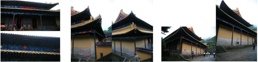

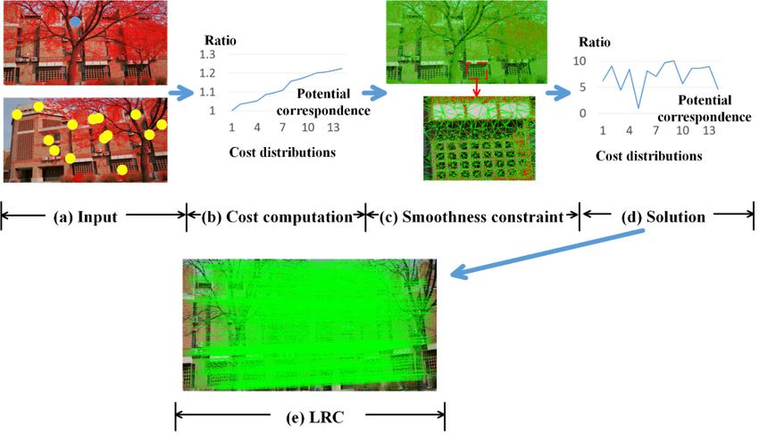
Remote Sens. 2020, 12, 3158 4 of 19

feature. The core algorithm formulates the feature matching as the optimization of a global energy
function based on a graph, which takes each feature point as nodes and defines the spatial
relationships (i.e., edges) of these nodes through Delaunay meshing [37]. The solut7ion of the energy
function is the final matching result of the proposed method. In general, the workflow of the
proposed method follows an iterative manner (Figure 1): (1) detect feature points in stereo images,
compute their intensity features using a certain feature descriptor (e.g., SIFT and SURF in this paper),
and find several potential correspondences for each feature in the basic through KD-tree [38] by
ranking their distances in the feature space, as shown in Figure 1a; (2) formulate these distances in
the feature space as the matching cost terms of the energy function, and each feature in the basic has
a series of matching cost with respect to its potential correspondences, as shown in Figure 1b, where
the maximum cost among the potential correspondences is only 1.23 times larger than the minimum
cost; (2) define the spatial relationships of these feature points through Delaunay meshing (as shown
in Figure 1c), impose smoothness constraints between adjacent feature points, and formulates these
constraints as the smoothness terms of the energy function, (3) break the optimization of the global
energy function into sub-optimizations of each feature point, and iteratively compute the local
solutions of these sub-optimizations so that the matching uncertainties in the matching cost can be
reduced, as shown in Figure 1d, where the second minimum cost is 4.45 times larger than the
minimum cost; (4) take the other image as the basic, repeat step (1) to (3), and detect and eliminate
mismatches through the left-right-consistency (LRC) strategy. The final remaining matching points
are shown in Figure 1e.

 Figure 1. The workflow of the proposed method. In (a), red dots show the feature points in stereo
 pairs, the blue and the yellow circles represent a feature point in the basic image and its potential
 correspondences in the other, respectively. In (b) and (d), the horizontal axis represents the index of
 the potential correspondences, and the vertical axis represents the ratio between the matching cost at
 a certain correspondence index and the minimum cost of the feature point; in (c), the red dots are
 feature points, and the green edges of the triangle meshes define the spatial relationships of these
 feature points; in (e), the green lines connect matches of the proposed method after the LRC strategy.

2.2. Feature Point Graph
 To impose the spatial smoothness constraints in the feature matching, each feature point needs
to first find its surrounding feature points. To achieve this goal, Delaunay meshing is used to connect
all feature points in the triangularization form, as shown in Figure 2a,b. The feature points and the
edges in the Delaunay mesh construct a graph = ( , ) with being the set of nodes/feature

Remote Sens. 2020, 12, 3158 5 of 19

points and being the set of edges. The matching result optimization of each feature point will be
influenced by its connected feature points. However, not all connected feature points can be used for
matching optimization. For example, some feature points have high uncertainties in their matching
cost, thus may propagate the uncertainties to other feature points through the edges. To address this
issue, the edges starting from the high-uncertainty/low-confidence feature points should be limited,
and the edges starting from the low-uncertainty/high-confidence feature points should be connected,
thus constructing a bidirectional graph (Figure 2c), where each edge has two weights with respect to
different directions. The weights of each edge will be described in Section 2.3. Each node in the graph
has a series of potential corresponding points, as shown in Figure 2d. Therefore, the final point feature
graph is a 3D discrete, irregular, bidirectional volume.

 Figure 2. Feature point graph. Blue circles are feature points or nodes in the graph; red lines are edges
 in the graph; yellow circles are potential corresponding points. (a) is the set of feature points with
 blue circles being nodes in the graph; (b) is the Delaunay meshing results from these feature points
 with red lines being edges in the graph; (c) shows bidirectional edges between feature points; (d)
 shows the potential corresponding points (the yellow circles) of each feature point.

2.3. Graph-Based Energy Function
 To find good corresponding points from the potential ones, this paper imposes the spatial
smoothness constraints between any two connected feature points with the underlying assumptions
that feature points should have similar matching results to their surrounding high-confidence points,
and formulates the feature matching problem as the minimization of an energy function based on the
feature point graph = ( , ). In general, the energy function consists of two terms: (1) cost term,
which measures the feature similarity between feature points and their potential corresponding
points, and (2) smoothness term, which penalizes the inconsistent matching results between any two
connected feature points. The formulation of the energy function is as follows.
 ( ) = ( , ) + ( , ) ∙ || − || /|| − ||
 ∈ , ∈ 
 (1)
 = − 
 = − 
 where, is the energy function; is the set of matching results (i.e., the correspondence ID)
of all feature points in the basic image; ( , ) is the matching cost of the feature point at its
potential correspondence label ; is the set of feature point in the other image; is the
potential corresponding point of at label ; || ∙ || measures the vector norm; measures the
disparities of in both row and column directions; , is an edge from to ; ( , ) is the
weight of the edge , , which is also termed as the penalty coefficient. It means the contribution of
 in the matching of . Since is a bidirectional graph, ( , ) and ( , ) often have different
values, which helps to reduce the influence of low-confidence points on the matching optimization.
To improve the matching robustness in slanted regions, the disparity difference || − || is
divided by || − || for the purpose of the normalization.
 In this paper, the cost term ( , ) computes the feature similarity between the feature point
 and its potential corresponding point by measuring their distance in the feature space.
There are various feature descriptors, among which SIFT [26] and SURF [27] are adopted in the
experimental comparisons in Section 4. However, the sizes of different feature descriptors are not the

Remote Sens. 2020, 12, 3158 6 of 19

same, thus leading to different matching cost ranges. To increase the generality of the proposed
method, this paper normalizes the matching cost by dividing it by the maximum matching cost, as
follows.
 , = || ( ) − ( )|| / 
 = max { ( , )} (2)
 ∈
 where, is a certain feature descriptor (e.g., SIFT or SURF in this paper); is the maximum
matching cost among the matching cost of ; is the number of potential correspondences.
The final feature matching optimization results of the proposed method partly depend on the number
of potential correspondences. Too small a number may exclude the true label, while too large a
number significantly increases the time cost of the feature matching. In this paper, the appropriate
correspondence number will be analyzed in Section 4.1.
 The smoothness term guides the matching results of any two connected feature points consistent
by penalizing the inconsistent cases. The matching result consistency is measured by the distances
between their disparity vectors in both row and column directions. Shorter distances mean more
consistent matching results as well as smaller penalties, and vice versa. However, some feature points
with low matching confidence may give bad influences on the matching of its surrounding feature
points. Therefore, the penalty coefficient of edges starting from these low-confidence feature
points should be reduced. In addition, the penalty coefficient is also related to the spatial distance
between the connected feature points. Considering matching in slanted regions, larger distance
should correspond to smaller , and vice versa. Therefore, the penalty coefficient ( , ) is a
function with two independent variables: (1) the matching confidence of and (2) the spatial
distance between and , as follows:
 , = ∙ + /|| − ||
 (3)
 = 1 − / 
where, is a predefined initial penalty coefficient; is the matching confidence of , which is
formulated as the ratio between the minimum matching cost and the second minimum
matching cost ; , are predefined parameters, which are used to increase the penalty
coefficient of high-confidence points and decrease the ones of low-confidence points. , adopt
fixed values in all experiments with = 0.4 and = 3 . defines the scale of the penalty
coefficient. In this paper, the appropriate values of will be analyzed in Section 4.2.

2.4. Solution
 The solution of the global energy function in Equation (1) is the final feature matching result.
However, the optimization of Equation (1) is a typical NP-hard problem, which means that its global
solution has high time complexity. For efficient computation purposes, a compromise solution of
Equation (1) is computed by splitting the global optimization into a collection of sub-optimizations
and then iteratively computing the local minimum for the matching of each feature point. To achieve
this goal, Equation (1) is first transformed into the summation of the local functions in Equation (4).
 ( ) = , )
 ∈ 
 (4)
 , ) = ( , ) + ( , ) ∙ || − || /|| − ||
 , ∈ 
where, is the set of edges that only end at ; , ) is a sub-optimization function which
only considers the cost term of and the smoothness term of edges that ends at .
 For computational purposes, this paper only computes the local solution of the sub-optimization
 , ) instead of the global optimal solution of ( ) , i.e., transform the energy function
min ( ) into ∑ ∈ min ( , , ) , which can greatly reduce the variable space. In the sub-
optimization of , ), the matching result of the connected points in is assumed available
so that the matching of is constrained by the connected, high-confidence points, as follows.
 = argmin , ) = argmin ( , ) + ( , ) ∙ || − || /|| − || (5)
 , ∈ 
where, is the initial matching result of the connected point .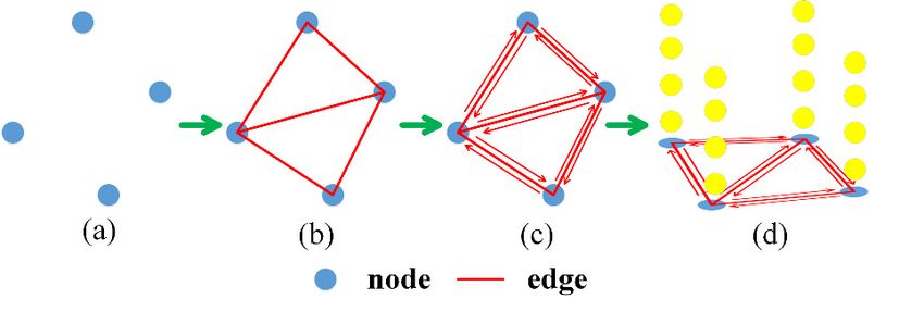

Remote Sens. 2020, 12, 3158 7 of 19

 The matching result of partly depends on . However, due to some geometric distortions
and weak/repeat textures, the initial matching result may be unreliable. To further improve the
matching accuracy, the sub-optimization in this paper proceeds in an iterative manner: (1) find the
corresponding point, for each feature point in the basic image, with the minimum matching cost as
the initial matching results; (2) compute the local optima of the matching for each feature point by
considering the initial matching results of their connected points, as shown in Equation (5); (3) update
the initial matching results and the matching cost with the local optima and the more reliable cost
 , respectively, and then detect the number of inliers from the optimal solutions by using the
fundamental matrix; (4) repeat step (2) to (3) until the inlier number in the current iteration is smaller
than the one in the previous iteration; (5) output the matching results with the most inliers. The
iterative sub-optimization manner is summarized as the pseudo-code in Algorithm 1.

 Algorithm 1: The iterative solution of the sub-optimization in the proposed method
 Function: Iterative_solution_of_sub_optimizations (PB, POther, , , )
 Input: the set of feature point in the basic image PB, the set of feature point in the other image POther, the set
 of connected points for each feature point in the basic image ; the set of matching cost of all feature point
 C;
 Output: the set of matching results of all feature points in the basic image 
 Pseudo-code:
 1. //step1: find the initial correspondence with the minimum matching cost
 2. for =1 to Num, do //Num is the feature point number in the basic
 3. ( ) = argmin ( , ) // ( ) is the initial matching result of the feature point i
 4. end for
 5. inlier_num_crt = Detect_inliers_using_Fundamental_matrix (PB, POther, )
 6. inlier_num_before = 0
 7. inlier_num_max = inlier_num_crt
 8. = 
 7. while (inlier_num_crt > inlier_num_before)
 8. {
 9. //step2: compute the local optima of the matching in Equation (5)
 10. for =1 to Num, do
 11. // ( ) is the new matching result of constrained by its surrounding connected points 
 12. //U(i) is the optimized matching cost after the local optimization
 13. [ ( ), U(i)] = Local_optima_of_matching (C, , , ( ))
 14. end for
 15. //step3: update the matching results as well as the matching cost
 16. = 
 17. = U
 18. inlier_num_before = inlier_num_crt
 19. inlier_num_crt = Detect_inliers_using_Fundamental_matrix (PB, POther, )
 20. //update the output matching result
 21. if (inlier_num_crt > inlier_num_max)
 22. inlier_num_max = inlier_num_crt
 23. = 
 24. end if
 25. }

 To remove mismatches in the matching results, this paper adopts the left-right-consistency check
(LRC) strategy. In general, this paper respectively takes the left and the right images as the basic finds
the corresponding points for each feature in the basic images by using the proposed method,
compares these two matching results, and detects and removes the inconsistent part whose matching
inconsistency is larger than 2 pixels. The matching inconsistency is measured by computing the
distance between the original feature point in the left and the matching result of its corresponding
point in the right, as follows.
 = || − ′||
 (6)
 = ′( ) ′ = ( )

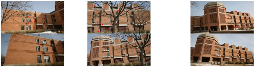
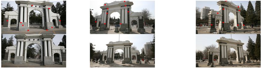
Remote Sens. 2020, 12, 3158 8 of 19

where, is a feature point in the left; is the corresponding point of when the left is the basic
image; is the correspondence label of when the right is the basic image; ′ is the
corresponding point of ; is the distance between and ′.

3. Study Areas and Data
 The proposed method was tested on close-range datasets provided by the National Laboratory
of Pattern Recognition, Institute of Automation, Chinese Academy of Science, including the Tsinghua
gate dataset, Bioscience building dataset, Fayu temple dataset, and the Zhantan temple dataset [39].
All datasets were captured by Canon EOS 5D. To evaluate the matching performance of the proposed
method, especially in large geometric-distortion and weak/repeat texture regions, this paper
respectively selected three pairs from each dataset with large scale differences (e.g., Figure
3(a1,b2,c1)), large perspective distortions (e.g., Figure 3(a2,b3,c3,d1,d2)), occlusions by pedestrians,
trees or other man-made objects (Figure 3(a3,c2,d2)) and weak/repeat textures (Figure 3b,c). The
limiting factors in most pairs are the combinations of multiple above distortion and texture factors.
To evaluate the matching accuracy of the proposed method, this paper manually selected nine
matching points as checking points for each image pair. The distributions of checking points on each
image pair are shown as red circles in Figure 3.

 (a2) Pair 2
 (a1) Pair 1 (a3) Pair 3
 Fayu temple dataset

 (b2) Pair 2
 (b1) Pair 1 (b3) Pair 3
 Tsinghua gate dataset

 (c2) Pair 2
 (c1) Pair 1 (c3) Pair 3
 Bioscience building dataset

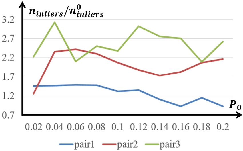
Remote Sens. 2020, 12, 3158 9 of 19

 (d2) Pair 2
 (d1) Pair 1 (d3) Pair 3
 Zhantan temple dataset

 Figure 3. The close-range datasets for experimental analysis and comparisons.

4. Results
 The proposed method was used to optimize the matching results of SIFT and SURF, termed SIFT
+ RMSS and SURF + RMSS, respectively. For fair comparisons, all matching methods (SIFT, SURF,
SIFT + RMSS, and SURF + RMSS) utilized the LRC strategy to detect and eliminate the mismatches,
and the remaining matching points were used in the experimental analysis and comparisons. The
matching accuracy of the proposed methods as well as other feature matching methods was
evaluated in three aspects: (1) the number of inliers , which measures the robustness of the
matching methods, especially in large-geometric-distortion regions and weak/repeat texture regions,
(2) the percentage of inliers , which measures the uncertainties in the matching results of each
method, and (3) the matching accuracy against the checking points (also termed absolute
accuracy). Matching points of each method were first utilized to compute a fundamental matrix
through a RANSAC strategy [40]. The number of inliers is counted by computing the
epipolar lines of matching points through the fundamental matrix and adopting the matching points
with the distances to the epipolar lines smaller than 2 pixels as inliers. The percentage of inliers
 is then formulated as the ratio between the number of inliers and the number of all matching
points. On the other hand, the absolute matching accuracy using checking points was
formulated as the average distance to the epipolar lines of all checking points.
 In general, this paper firstly analyzed some parameters of the proposed method on the Fayu
temple dataset, i.e., the number of the potential correspondences in Section 4.1 and the initial penalty
coefficient in Section 4.2, by studying the matching accuracy (including the inlier number , the
inlier percentage and the absolute matching accuracy ) with various parameters, and
found the most appropriate parameters with the highest matching accuracy. Then, the proposed
method was used to optimize the matching results of SIFT and SURF on the Tsinghua gate dataset,
Bioscience building dataset, and Zhantan temple dataset, and the optimized matching results were
compared with the original matching results as well as a robust matching method via vector field
consensus (VFC) [35] in the aspects of , and in Section 4.3. VFC solved for
correspondence by interpolating a vector field between the two feature point sets and imposed
nonparametric geometrical constraints in the vector field to obtain good matches. All experiments
were conducted on the same compute configuration with a single CPU @ 2.60GHz.

4.1. Analysis About the Influence of the Number of the Potential Correspondences on the Final Matching
Results
 The matching results of the proposed method partly depend on the number of potential
correspondences (i.e., in Equation (2)). Too small a number may exclude the true
correspondence, while too large a number will increase the time cost. To select appropriate number
of the potential correspondences, this paper firstly utilized the proposed method to optimize the
matching results of SIFT on the Fayu temple dataset and then analyzed the matching accuracy of the
proposed method in the metrics of the inlier number , the inlier ratio and the

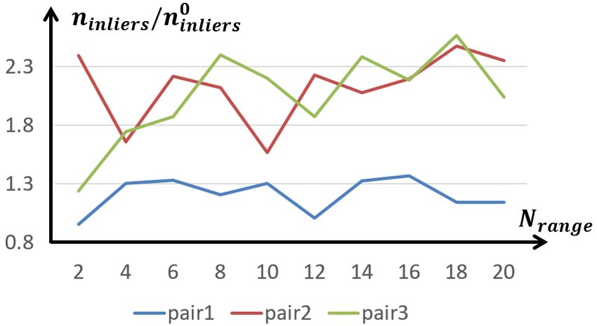
Remote Sens. 2020, 12, 3158 10 of 19

absolute matching accuracy with various Nrange (from 2 to 20). As the ranges of the metrics in
different pairs may be significantly different (e.g., some pairs have hundreds of inliers, while some
only have dozens of inliers), this paper normalized the matching accuracy of the proposed method
by dividing it by the matching accuracy of SIFT (termed , and , respectively)
so that the normalized matching accuracy on different pairs were at the same level, as shown in
Figure 4. / in Figure 4a and / in Figure 4b are the ratio between the
number of inliers of the proposed method and SIFT, and the ratio between the percentages of inliers
of the proposed method and SIFT, respectively, thus the larger ratio / (> 1) and
 / (> 1) mean more robust matching results. / in Figure 4c is the ratio
between the absolute matching accuracy of the proposed method and SIFT, thus smaller ratio
 / (< 1) means higher matching accuracy.

 (a) Number of inliers

 (b) Percentage of inlier

 (c) Absolute matching accuracy

 Figure 4. The trend of matching accuracy with various Nrange on the Fayu temple dataset. (a) shows
 the inlier number trend with increasing Nrange; (b) shows inlier percentage trends with increasing Nrange;
 (c) shows the absolute matching accuracy trends with increasing Nrange.

Remote Sens. 2020, 12, 3158 11 of 19

 In Figure 4a, almost all number ratios / on all pairs are larger than one (except for
pair 1 with as two), which means that the inlier number of SIFT has been increased after the
optimization of our proposed method. In Figure 4b, all percentage ratios / are
larger than one, which means that the inlier percentages of the proposed methods were also higher
than SIFT. Therefore, the proposed method can provide more robust feature matching results for the
later camera orientations. The percentage ratio / has an increasing trend with the
increasing of Nrange, since larger Nrange means a lower probability of selecting the same matching
results for the mismatches. More robust matching results (higher inlier number and higher inlier
percentage) can often be used to compute higher-accuracy camera orientation results, thus all
absolute accuracy ratio / in Figure 4c are smaller than 1. Figure 4 shows that the
proposed method could achieve higher matching accuracy, though Nrange varied greatly. To achieve
the highest matching accuracy, the most appropriate Nrange is needed to be selected in the feature
matching. However, different pairs corresponded to different appropriate Nrange in different matching
accuracy metrics, e.g., the most appropriate of pair 1 are 16, 16, and 18, respectively, in the
metrics of , and , while the most appropriate ones of pair 2 are 18, 18, and 12,
respectively, in the metrics of , and . To give a comprehensive evaluation of
 , this paper, therefore, ranked the matching accuracy of each pair, as shown in Equation (7),
and then summarized these ranks to find the most appropriate Nrange with respect to the highest
ranking, as shown in Figure 5.
 , / , ( ) = 
 , ( )= (7)
 , ( )/ , = 
where, represents a certain stereo pair; represents a certain matching accuracy metric;
 , ( ) means the matching accuracy of pair in the metric of at a certain Nrange;
 , ( ) means the rank of pair in the metric of at a certain Nrange; , means the
maximum value of matching accuracy among various Nrange, while , means the minimum value
of matching accuracy among various Nrange. , closer to one means higher matching accuracy.
The summation of all ranking results is shown as follows.

 Figure 5. Ranking with various on the Fayu temple dataset.

 In Figure 5, a shorter-length bin means higher ranking. The ranking results did not change much
when Nrange ≥ 10, which shows that such a number of potential correspondences is sufficient to
include the true correspondence. The red bin with Nrange as 14 has the highest ranking. Therefore, this
paper adopted Nrange = 14 in all the following experiments in Section 4.2 and 4.3.

4.2. Analysis About the Influence of the Initial Penalty Coefficient on the Final Matching Results
 In addition to the number of the potential correspondences Nrange, this paper also evaluated the
influences of the initial penalty coefficient (i.e., in Equation (3)) on the feature matching accuracy.
Too small will bring weak smoothness constraints so that the matching of each feature point
cannot be optimized by its surrounding points. On the other hand, too large will decrease the
contribution of the matching cost in the feature matching process so that some mismatches will be

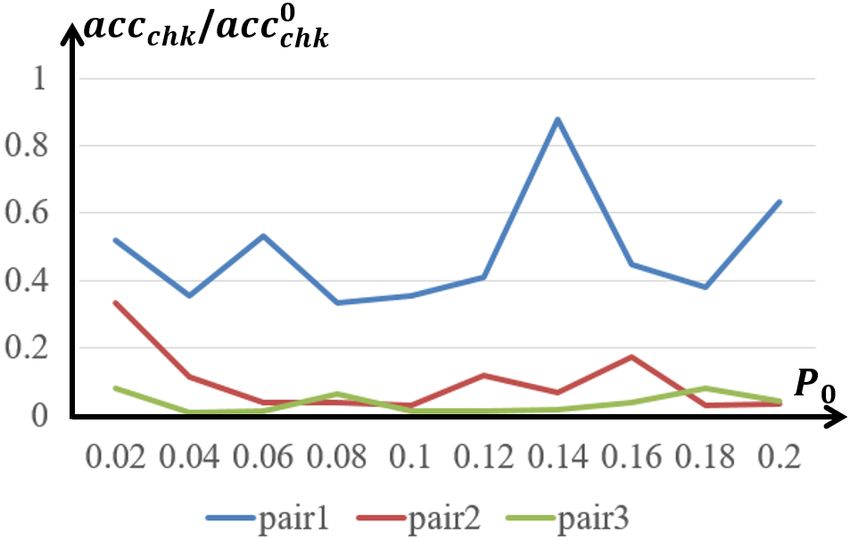
Remote Sens. 2020, 12, 3158 12 of 19

generated in some slanted regions or height jumps. To select appropriate , this paper still utilized
the proposed method to optimize the matching results of SIFT on the Fayu temple dataset with various
 (from 0.02 to 0.2), and then analyzed the matching accuracy of the proposed method in the metrics
of the inlier number , the inlier ratio and the absolute matching accuracy . For
better experimental comparisons, this paper also normalized the matching accuracy of the proposed
method by dividing it by the matching accuracy of SIFT (termed , and ,
respectively). The experimental comparisons on various are shown in Figure 6.

 (a) Number of inliers

 (b) Percentage of inlier

 (c) Absolute matching accuracy

 Figure 6. The trend of matching accuracy with various on the Fayu temple dataset. (a) shows the
 inlier number trend with increasing ; (b) shows inlier percentage trends with increasing ; (c)
 shows the absolute matching accuracy trends with increasing .

 In Figure 6a, most inlier number ratios / are larger than one (except for pair 1 with
 as 0.16 and 0.2, respectively), which shows that the matching results of the proposed method is
robust against the variation of when < 0.16. However, too large (e.g., ≥ 0.16) may
decrease the inlier number, since such large may bring over-smoothness constraints in the feature
matching. In Figure 6b, all percentage ratios / are larger than one, which means
that the matching results of the proposed method contained more inliers as well as fewer outliers
than SIFT. All absolute accuracy ratio / in Figure 6c are smaller than 1, which means
that the proposed method is capable of greatly improving the matching accuracy of SIFT. The highest

Remote Sens. 2020, 12, 3158 13 of 19

matching accuracy improvement on the three pairs were 66.44% at = 0.08, 96.99% at = 0.18
and 98.89% at = 0.04, respectively. Therefore, the most appropriate for different pairs were
different. To select the most appropriate in a general scenario, this paper still ranked the matching
accuracy of each pair in Equation (7) and then summarized these ranks to find the most appropriate
 with respect to the highest ranking, as shown in Figure 7.

 Figure 7. Ranking with various on the Fayu temple dataset.

 In Figure 7, the ranking results did not change much when 0.04 ≤ ≤ 0.14, which shows that
such a range of the initial penalty coefficient is appropriate for the proposed method on the matching
optimization of SIFT. The red bin with as 0.1 has the highest ranking. Therefore, this paper
adopted = 0.1 in all the following experiments in 3.3.

4.3. Matching Accuracy Comparisons on more Datasets
 To give more comprehensive evaluations of the proposed method, this paper applied SIFT [26]
and SURF [27] on more datasets (i.e., Tsinghua gate dataset, Bioscience building dataset, and Zhantan
temple dataset), utilized the proposed method to optimize the matching results of SIFT and SURF,
respectively, and compared the proposed method with a state-of-the-art matching method VFC [35].
VFC improved the matching results of SIFT or SURF by interpolating a vector field between the two
feature point sets and imposed nonparametric geometrical constraints in the vector field. The final
matching results of VFC and the proposed method are termed as SIFT + RMSS, SURF + RMSS, SIFT
+ VFC, and SURF + VFC. All stereo pairs in the testing datasets were 4368×2912 pixels. Matching
parameters of the proposed method were fixed by using the experimental conclusions in Section 4.1
and 4.2, i.e., = 14 and = 0.1. The matching accuracy of SIFT, SURF, SIFT + VFC, SURF +
VFC, SIFT + RMSS, and SURF + RMSS were also evaluated in the three metrics, i.e., the inlier number
 , the inlier ratio and the absolute matching accuracy . The running time of
these methods was also tested. The experimental comparisons about the matching accuracy and the
running time are shown in Figure 8. The horizontal axes mean the ID of stereo pairs in the Tsinghua
gate dataset, Bioscience building dataset, and Zhantan temple dataset in Figure 3, and the vertical
axes mean the matching accuracy in Figure 8a–c, and the running time in Figure 8d. However, the
ranges of the absolute accuracy of different matching methods on different pairs were significantly
different. For better comparisons, this paper truncated absolute accuracy values that were larger than
100 pixels, and then divided all absolute accuracy values of a certain pair by ten as long as any one
of the absolute accuracy values was larger than ten. Since the testing datasets were of poor matching
quality (e.g., large geometric distortions, weak/repeat textures and occlusions) for SIFT and SURF,
most pairs needed the absolute accuracy division operator except for the pair c-2 (marked by * in
Figure 8c).

Remote Sens. 2020, 12, 3158 14 of 19

 (a) Inlier number (b) Inlier percentage

 (c) Absolute matching accuracy (d) Running time

 Figure 8. Experimental comparisons among SIFT, SURF, VFC, and the proposed method

 Figure 8a shows the inlier number of SIFT, SURF, SIFT + RMSS, and SURF + RMSS on all testing
datasets. VFC generally increased the inlier number of SIFT and SURF by average 44.7% and 59.3%,
respectively, while its matching results were not robust. In some cases (e.g., SIFT + VFC in b-1 and
SURF + VFC in d-3), the inlier number after VFC was even less than the original ones. On the other
hand, the inlier number of SIFT and SURF has been increased by the proposed method in all cases,
which shows that the proposed method can robustly reduce the matching uncertainties in SIFT and
SURF by imposing the smoothness constraints. After the optimization of the proposed method, the
SIFT/SURF matching points can be increased by at most 437.5%/272.9%, at least 15.7%/5.5%, and
average 131.9%/113.5%. In Figure 8b, the average inlier percentages of SIFT and SURF were only as
low as 10.5% and 6.9%, respectively, due to the large geometric distortions, weak/repeat textures, and
occlusions in the testing datasets. VFC can significantly improve the inlier percentages of SIFT and
SURF to average 25.0% and 28.0%, respectively. However, VFC still met the unstable problem in some
cases (e.g., SIFT + VFC in b-1), where the inlier percentages of VFC were lower than the original ones.
The proposed method could improve the inlier percentage in all cases. After the optimization of the
proposed method, the average inlier percentages of SIFT + RMSS and SURF + RMSS can be increased
to 37.7% and 28.1%, respectively. It shows that the proposed method can also reduce the mismatches
as well as increase the inliers in the matching results as the proposed method considers more
potential correspondences in the matching and imposes the smoothness constraints to reduce the
matching uncertainties. Though the general performance of VFC was not as good as the proposed
method, it could achieve better results in some cases (e.g., c-2). In Figure 8c, the proposed method
can significantly improve the absolute matching accuracy of SIFT/SURF by at most 97.9%/96.1%, at
least 55.2%/-0.65%, and average 80.6%/70.2%. The proposed method is capable of improving the
absolute matching accuracy in most cases except for the SURF matching of pair c-2. It is because the
matching results of SURF on pair c-2 were already good with 3471 inliers, in which case the proposed
method did little to such a good matching result. The unstable inlier number and the inlier percentage

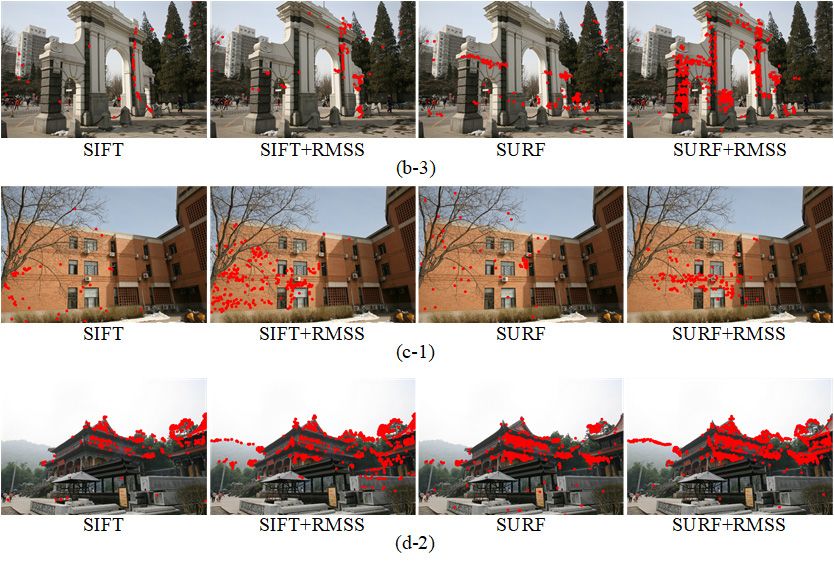
Remote Sens. 2020, 12, 3158 15 of 19

of VFC resulted in unstable absolute matching accuracy. In some cases (e.g., SURF + VFC in b-3), it
can significantly improve the absolute matching accuracy by 94.9%, while in some cases (e.g., SIFT +
VFC in c-1), it might decrease the absolute matching accuracy by 44.1%. In general, the proposed
method can greatly improve the matching results of SIFT and SURF on poor-quality stereo pairs.
Since the proposed method optimized the matching results of SIFT and SURF in an iterative manner,
the running time of the proposed method was certainly longer than the pure SIFT or the pure SURF.
The proposed method added on average 25.3 s more time to the SIFT matching and 52.3 s more time
to the SURF matching on the testing datasets. VFC was much more efficient than the proposed
method with 61.3% and 73.0% less time cost for SIFT and SURF, respectively. It should be noted that
VFC was even faster than pure SIFT and pure SURF. It is because VFC has already been capable of
removing mismatches, therefore it could avoid the repeat computation of the LRC strategy.
Considering only one single CPU is used in the proposed method, it has great potential to speed up
when a parallel framework is applied.
 To give more visual comparisons, this paper selected pairs with the least inliers from each testing
dataset (i.e., (b-3), (c-1), and (d-2)), and illustrated the inliers of SIFT, SURF, SIFT + RMSS, and SURF
+ RMSS, respectively, as shown in Figure 9. Since Fayu temple dataset (Figure 3(a1–a3)) is a training
dataset, which is used to train matching parameters of the proposed method, we did not illustrate the
matching results on such dataset for fair comparisons.

 Figure 9. Inliers distributions before/after the optimization of the proposed method. (b-3) is the
 stereo pair with the least inliers in Tsinghua gate dataset; (c-1) is the stereo pair with the least inliers
 in Bioscience building dataset; (d-2) is the stereo pair with the least inliers in Zhantan temple dataset.

 In Figure 9, the weak textures of the white wall in b-3, and the repeat textures of the black wall
in (b-3) and the yellow wall in c-1 brought high matching uncertainties in SIFT and SURF. Thus, both
methods only matched dozens of points. The proposed method-imposed smoothness constraints to
reduce the matching uncertainties, thus being able to achieve more matching points in weak texture
and repeat texture regions. In Figure 9(d-2), the matching points of SIFT and SURF only concentrated
on the roof of the temple. The uneven distributions of matching points may lead to low camera

Remote Sens. 2020, 12, 3158 16 of 19

orientation accuracy. The proposed method not only matched more points on the temple roof but
also matched more even points (e.g., the points on the mountain). In general, the proposed method
is capable of achieving more robust matching results than pure SIFT and pure SURF.

5. Discussion
 The results of this study indicate that the proposed method can greatly improve the matching
results of SIFT and SURF in some matching difficult regions (e.g., large geometric-distortion regions
and repeat textured regions). The experimental comparisons were tested on the datasets of Tsinghua
gate, Bioscience building, and Zhantan temple, which had serious matching limiting factors. Both
SIFT and SURF performed badly on the testing datasets with the average inlier number being
973.7/1072.2, the average inlier ratio being 10.5%/6.9% and the average absolute matching accuracy
being 27.0/27.5 pixels. As the proposed method reduces the matching uncertainties of feature points
by imposing spatial smoothness constraints over the whole feature point sets, it can greatly improve
the matching results of SIFT and SURF. After the optimization of the proposed method, the
corresponding accuracy was improved to 1549.9/1759.8, 37.7%/28.1%, and 4.09/2.89 pixels,
respectively. In addition to the matching accuracy improvement, the proposed method also
obviously increased the matches of SIFT and SURF, as shown in Figure 9. For example, Figure 9(b-
3,c-1) have repeat textures on the walls of the Tsinghua gate and Bioscience building, where
traditional SIFT and SUFR matched few points, due to the high matching uncertainties. The proposed
method introduced spatial smoothness constraints to reduce these uncertainties, thus achieving more
matches.
 The study has gone some way towards enhancing our understanding of feature matching with
spatial constraints. Before this, some spatial constraints-based matching (SCM) methods utilized seed
points to constrain the matching process, while the wrong seed points will give wrong matching clues
to the matching of other features, this may decrease the final matching accuracy. The proposed
method instead constrains the matching process through the optimization of the energy function,
thus being more fit for the matching in difficult regions. Therefore, the proposed method has a great
potential to be applied in some close-range and oblique photogrammetric applications, e.g., street-
view mapping, robot navigation, relic reconstruction, and city modeling.
 The proposed method has some limitations to be considered. First, the parameter selections in
Section 4.1 and 4.2 were determined through SIFT matching results and were also proved to be valid
for SURF matching in Section 4.3. However, since the descriptors of different matching methods may
be significantly different. The best parameters of SIFT and SURF may not be fit for other feature
descriptors. Therefore, it is recommended to retrain new matching parameters if other feature
descriptors were used. Second, the proposed method has a higher time cost than the pure SIFT and
SURF, and the time differences have an increasing trend with the increasing of feature points. For
example, the time cost of the proposed is 1.75 times higher than SIFT when the number of SIFT
features is 56,165, while the multiple reaches 3.25 when the number of SIFT features is 167,159. The
increasing multiple of time cost is caused by the Delaunay triangularization and the optimization of
the energy function in the proposed method. Therefore, the proposed method was not fit for the
scenarios with large amounts of feature points and high time efficiency demands. The above limiting
factors of the proposed method need to be further investigated in the future. We plan to enhance the
normalization of different feature descriptors so that the trained matching parameters could have
more general applicability. We also plan to improve the efficiency of the spatial relationship
determination of adjacent feature points by introducing tree-structure indexing.

6. Conclusions
 This paper aims at addressing the matching uncertainties issues in large geometric-distortion
regions, weak-texture regions, and repeat-texture regions, and proposes a robust feature matching
method with spatial smoothness constraints to reduce such uncertainties with the underlying
assumptions that each feature point should have a similar matching result to its surrounding high-
confidence points. The core algorithm formulates the feature matching as a minimization of a global

Remote Sens. 2020, 12, 3158 17 of 19

energy function based on a feature point graph and introduces a comprise solution by breaking the
optimization into a collection of sub-optimizations of each feature point. The proposed method is
capable of greatly optimizing the matching results of SIFT and SURF on some poor-quality stereo
pairs. Experiments on several poor-quality, close-range datasets show that the proposed method can
significantly increase the inliers number of SIFT and SURF by average 131.9% and 113.5%, improve
the inlier ratios of SIFT and SURF by average 259.0% and 307.2%, and improve the absolute matching
accuracy of SIFT and SURF by average 80.6% and 70.2%, respectively. However, the proposed method
will add more running time to the feature matching. For more efficient and more robust feature
matching, the authors plan to reduce the time cost by applying a parallel framework in the future.

Author Contributions: Conceptualization, X.H.; methodology, X.H.; software, X.H.; validation, X.H.; formal
analysis, X.H.; investigation, X.H. and X.W.; resources, X.H.; data curation, X.H.; writing—original draft
preparation, X.H. and X.W.; writing—review and editing, X.H. and D.P.; visualization, X.H. and D.P.;
supervision, X.H.; project administration, X.H.; funding acquisition, X.H. All authors have read and agreed to
the published version of the manuscript.

Funding: This research was funded by the National Natural Science Foundation of China (grant number
41701540), Basic Startup Funding of Sun Yat-sen University (grant number 76230-18841205), National Natural
Science Foundation of China (grant number 41801386), Innovation Program of CSU, CAS (grant number
Y8031831).

Acknowledgments: The authors would like to thank the National Laboratory of Pattern Recognition, Institute
of Automation, Chinese Academy of Science for providing the close-range dataset. The authors would like to
thank Yilong Han for calibrating camera distortions in the testing datasets.

Conflicts of Interest: The authors declare no conflict of interest.

References
1. Szeliski, R. Computer Vision: Algorithms and Applications, 1st ed.; Springer: Berlin, Germany, 2010; pp. 183–
 228.
2. Ling, X.; Huang, X.; Zhang, Y.; Zhou, G. Matching Confidence Constrained Bundle Adjustment for Multi-
 View High-Resolution Satellite Images. Remote Sens. 2020, 12, 20.
3. Huang, X.; Liu, W.; Qin, R. A window size selection network for stereo dense image matching. Int. J. Remote
 Sens. 2020, 41, 4836–4846.
4. Huang, X.; Hu, K.; Ling, X.; Zhang, Y.; Lu, Z.; Zhou, G. Global Patch Matching. In Proceedings of the ISPRS
 Annals of the Photogrammetry, Remote Sensing and Spatial Information Sciences, Wuhan, China, 18–22
 September 2017; pp. 227–234.
5. Liu, X.; Zhang, Y.; Ling, X.; Wan, Y.; Liu, L.; Li, Q. TopoLAP: Topology Recovery for Building
 Reconstruction by Deducing the Relationships between Linear and Planar Primitives. Remote Sens. 2019,
 11, 1372.
6. Ren, Z.; Meng, J.; Yuan, J. Depth camera based hand gesture recognition and its applications in Human-
 Computer-Interaction. In Proceedings of the International Conference on Information and Communication
 Security, Singapore, 13–16 December 2011; pp. 1–5.
7. Kim, Y.; Baek, S.; Bae, B. Motion Capture of the Human Body Using Multiple Depth Sensors. ETRI J. 2017,
 39, 181–190.
8. Kim, K.; Lawrence, R.L.; Kyllonen, N.; Ludewig, P.M.; Ellingson, A.M.; Keefe, D.F. Anatomical 2D/3D
 shape-matching in virtual reality: A user interface for quantifying joint kinematics with radiographic
 imaging. In Proceedings of the IEEE Symposium on 3d User Interfaces, Los Angeles, California, CA, USA,
 18–19 March 2017; pp. 243–244.
9. Kim, J.; Lin, S.; Hong, J.; Kim, Y.; Park, C. Implementation of Martian virtual reality environment using
 very high-resolution stereo topographic data. Comput. Geosci. 2012, 44, 184–195.
10. Wu, Y.; Di, L.; Ming, Y.; Lv, H.; Tan, H. High-Resolution Optical Remote Sensing Image Registration via
 Reweighted Random Walk based Hyper-Graph Matching. Remote Sens. 2019, 11, 2841.
11. Yang, H.; Li, X.; Zhao, L.; Chen, S. A Novel Coarse-to-Fine Scheme for Remote Sensing Image Registration
 Based on SIFT and Phase Correlation. Remote Sens. 2019, 11, 1833.

Remote Sens. 2020, 12, 3158 18 of 19

12. Wang, M.; Zhang, H.; Sun, W.; Li, S.; Wang, F.; Yang, G. A Coarse-to-Fine Deep Learning Based Land Use
 Change Detection Method for High-Resolution Remote Sensing Images. Remote Sens. 2020, 12, 1933.
13. Dong, H.; Ma, W.; Wu, Y.; Zhang, J.; Jiao, L. Self-Supervised Representation Learning for Remote Sensing
 Image Change Detection Based on Temporal Prediction. Remote Sens. 2020, 12, 1868.
14. He, F.; Zhou, T.; Xiong, W.; Hasheminnasab, S.M.; Habib, A. Automated Aerial Triangulation for UAV-
 Based Mapping. Remote Sens. 2018, 10, 1952.
15. Iacobucci, G.; Troiani, F.; Milli, S.; Mazzanti, P.; Piacentini, D.; Zocchi, M.; Nadali, D. Combining Satellite
 Multispectral Imagery and Topographic Data for the Detection and Mapping of Fluvial Avulsion Processes
 in Lowland Areas. Remote Sens. 2020, 12, 2243.
16. Wan, Y.; Zhang, Y.; Liu, X. An a-contrario method of mismatch detection for two-view pushbroom satellite
 images. ISPRS J. Photogramm. Remote Sens. 2019, 153, 123–136.
17. Wan, Y.; Zhang, Y. The P2L method of mismatch detection for push broom high-resolution satellite images.
 ISPRS J. Photogramm. Remote Sens. 2017, 130, 317–328.
18. Huang, X.; Qin, R. Multi-view large-scale bundle adjustment method for high-resolution satellite images.
 In Proceedings of the ASPRS Conference, Denver, CO, USA, 27–31 January 2019.
19. Tatar, N.; Arefi, H. Stereo rectification of pushbroom satellite images by robustly estimating the
 fundamental matrix. Int. J. Remote Sens. 2019, 40, 8879–8898.
20. Qin, R. RPC Stereo Processor (RSP): A Software Package for Digital Surface Model and Orthophoto
 Generation from Satellite Stereo Imagery. In Proceedings of the ISPRS Annals of the Photogrammetry,
 Remote Sensing and Spatial Information Sciences, Prague, Czechoslovakia, 12–19 July 2016; pp. 77–82.
21. Jiang, S.; Jiang, W. On-Board GNSS/IMU Assisted Feature Extraction and Matching for Oblique UAV
 Images. Remote Sens. 2017, 9, 813.
22. Hu, H.; Zhu, Q.; Du, Z.; Zhang, Y.; Ding, Y. Reliable Spatial Relationship Constrained Feature Point
 Matching of Oblique Aerial Images. Photogramm. Eng. Remote Sens. 2015, 81, 49–58.
23. Zhang, Y.; Xiong, X.; Zheng, M.; Huang, X. LiDAR Strip Adjustment Using Multifeatures Matched with
 Aerial Images. IEEE T. Geosci. Remote Sens. 2015, 53, 976–987.
24. Ling, X.; Zhang, Y.; Xiong, J.; Huang, X.; Chen, Z. An Image Matching Algorithm Integrating Global SRTM
 and Image Segmentation for Multi-Source Satellite Imagery. Remote Sens. 2016, 8, 672.
25. Duan, Y.; Huang, X.; Xiong, J.; Zhang, Y.; Wang, B. A combined image matching method for Chinese optical
 satellite imagery. Int. J. Digit. Earth 2016, 9, 851–872.
26. Lowe, D.G. Distinctive Image Features from Scale-Invariant Keypoints. Int. J. Comput. Vis. 2004, 60, 91–110.
27. Bay, H.; Tuytelaars, T.; Van Gool, L. SURF: Speeded up robust features. In Proceedings of the European
 Conference on Computer Vision, Graz, Austria, 12–18 October 2006; pp. 404–417.
28. Leutenegger, S.; Chli, M.; Siegwart, R. BRISK: Binary Robust invariant scalable keypoints. In Proceedings
 of the International Conference on Computer Vision, Barcelona, Spain, 6–13 November 2011; pp. 2548–
 2555.
29. Morel, J.; Yu, G. ASIFT: A New Framework for Fully Affine Invariant Image Comparison. SIAM J. Imag.
 Sci. 2009, 2, 438–469.
30. Fern, P.; Alcantarilla, N.; Bartoli, A.; Davison, A.J. KAZE features. In Proceedings of the European
 Conference on Computer Vision, Florence, Italy, 7–13 October 2012; pp. 214–227.
31. Sons, M.; Kinzig, C.; Zanker, D.; Stiller, C. An Approach for CNN-Based Feature Matching Towards Real-
 Time SLAM. In Proceedings of the International Conference on Intelligent Transportation Systems,
 Auckland, New Zealand, 27–30 October, 2019; pp. 1305–1310.
32. Zagoruyko, S.; Komodakis, N. Learning to compare image patches via convolutional neural networks. In
 Proceedings of the Computer Vision and Pattern Recognition, Boston, Massachusetts, US, 7–12 June, 2015;
 pp. 4353–4361.
33. Li, J.; Hu, Q.; Ai, M. 4FP-Structure: A Robust Local Region Feature Descriptor. Photogramm. Eng. Remote
 Sens. 2017, 83, 813–826.
34. Chen, M.; Qin, R.; He, H.; Zhu, Q., Wang, X. A Local Distinctive Features Matching Method for Remote
 Sensing Images with Repetitive Patterns. Photogramm. Eng. Remote Sens. 2018, 84, 513–524.
35. Ma, J.; Zhao, J.; Tian, J.; Yuille, A.L.; Tu, Z. Robust point matching via vector field consensus. IEEE Trans.
 Imag. Process. 2014, 23, 1706–1721.
36. Winter, M.; Ober, S.; Arth, C.; Bischof, H. Vocabulary Tree Hypotheses and Co-Occurrences. In Proceedings
 of the 12th Computer Vision Winter Workshop (CVWW’07), St. Lambrecht, Austria, 6–8 February 2007.