A Heuristic Angular Clustering Framework for Secured Statistical Data Aggregation in Sensor Networks - MDPI
←
→
Page content transcription
If your browser does not render page correctly, please read the page content below
sensors
Article
A Heuristic Angular Clustering Framework for
Secured Statistical Data Aggregation in
Sensor Networks
Lalitha Krishnasamy 1 , Rajesh Kumar Dhanaraj 2 , D. Ganesh Gopal 2 ,
Thippa Reddy Gadekallu 3 , Mohamed K. Aboudaif 4, * and Emad Abouel Nasr 5,6
 1    Department of IT, Kongu Engineering College, Tamil Nadu- 638060, India; klalitha.it@kongu.edu
 2    School of Computing Science & Engineering, Galgotias University, Uttar Pradesh 203201, India;
      d.rajeshkumar@galgotiasuniversity.edu.in (R.K.D.); dganeshgopal@gmail.com (D.G.G.)
 3    School of Information Technology and Engineering, VIT-Vellore, Tamil Nadu 632014, India;
      thippareddy.g@vit.ac.in
 4    Advanced Manufacturing Institute, King Saud University, Riyadh 11421, Saudi Arabia
 5    Industrial Engineering Department, College of Engineering, King Saud University,
      Riyadh 11421, Saudi Arabia; eabdelghany@ksu.edu.sa
 6    Mechanical Engineering Department, Faculty of Engineering, Helwan University, Cairo 11732, Egypt
 *    Correspondence: maboudaif@ksu.edu.sa

 Received: 20 July 2020; Accepted: 29 August 2020; Published: 31 August 2020

 Abstract: Clustering in wireless sensor networks plays a vital role in solving energy and scalability
 issues. Although multiple deployment structures and cluster shapes have been implemented, they
 sometimes fail to produce the expected outcomes owing to different geographical area shapes.
 This paper proposes a clustering algorithm with a complex deployment structure called radial-shaped
 clustering (RSC). The deployment structure is divided into multiple virtual concentric rings, and each
 ring is further divided into sectors called clusters. The node closest to the midpoint of each sector is
 selected as the cluster head. Each sector’s data are aggregated and forwarded to the sink node through
 angular inclination routing. We experimented and compared the proposed RSC performance against
 that of the existing fan-shaped clustering algorithm. Experimental results reveal that RSC outperforms
 the existing algorithm in scalability and network lifetime for large-scale sensor deployments.

 Keywords: clustering; radial-shaped clustering; node deployment; energy efficiency; routing;
 sensor networks

1. Introduction
      In most applications, sensors are used on a large scale to improve reliability and efficiency.
A wireless sensor network (WSN) comprises a large number of sensor nodes with sensing and
communication capabilities. The sensor nodes jointly collect and transmit data to the coordinator
node, referred to as the sink node [1]. The main objective of deploying sensor nodes is to monitor the
surrounding phenomenon, then process and transfer information to an analysis center. Sensor nodes are
static, mobile devices commonly powered by limited power sources like batteries [2–6]. Sensor nodes
have a limited transmission range. Consequently, optimal power utilization and the transmission of
data over long distances is essential in a network of sensor nodes.
      In a network of sensor nodes, clustering techniques are used for data collection, where sensor
nodes are grouped into clusters for the conservation of energy [7]. Each cluster consists of nodes
called members and a frequent reporting point called the cluster head (CH). Each node senses data
and transmits them to their corresponding CH. Subsequently, the CH aggregates the collected data,

Sensors 2020, 20, 4937; doi:10.3390/s20174937                                   www.mdpi.com/journal/sensors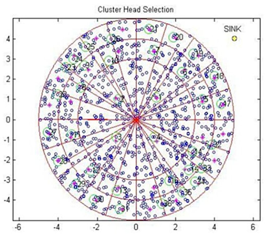
Sensors 2020, 20, 4937                                                                            2 of 15

converts them to a single tiny packet, and sends it to the sink node. Implementing the clustering
technique reduces the network load and conserves energy, and makes the nodes live.
      Clustering, based on the size and shape of the deployment area, is a method adopted commonly
to collect and transmit data to reduce energy consumption considerably. In previous research that
has been studied, various clustering techniques have been identified to improve energy efficiency in a
network of sensor nodes. However, most of the deployment structures adopted are either square or
rectangular in shape. The square or rectangular-shaped structures might produce satisfactory results
during simulation, but they are not suitable for all geographical regions for real-time deployment.
      In real-time applications, square-shaped sensors are not often deployed. For example, in airports,
sensors are deployed in the passenger lobbies and runway paths, which are often irregular in shape.
In weather stations also, sensors are deployed randomly in specific areas that are irregular in shape,
based on the transmission range. Therefore, there is a need for an algorithm capable of adapting to any
geographic region with different deployment structures.
      The security of sensor nodes and the data collected from the sensors that has to be transmitted
securely to the sink or another network is another challenging issue, in addition to the deployment
structure and cluster optimization. The intruders play a major role for spoofing the data in the middle.
Many research algorithms and techniques were implemented to address the security issues like artificial
intelligence mechanisms, multiagent schemes and artificial intelligent bots, etc. [8].
      Although attention has been given to the deployment structure, energy optimization in sensor
nodes poses a significant challenge in WSNs. In recent years, several clustering approaches have
been aimed at addressing the efficient energy consumption issues in WSNs [4,5,9–12]. In most of the
existing works, including LEACH [9], HEED [10], PEGASIS [13], enhanced LEACH and GBCR [14],
and SPIN [15], the CH is selected based on the highest residual energy and the CH to CH data
transmission is based on the coverage range and energy level. The selection and data transmission
between CHs are based only on the energy levels and it could increase the number of hops from a CH
to the sink node. The CH located closest to the mid area and angular-based routing can minimize the
number of hops from the CH to the sink node.
      The major contributions of this work are:

•     to determine the shape of the deployment area and the coverage range based on the network area
      to ensure that no node is left unattended and
•     to select the CH with energy optimization to achieve a balanced WSN with minimal
      energy requirements.

2. Related Works
     Clustering and routing are the fundamental processes in WSNs, and subsequent improvements
have been made to the LEACH protocol. The cluster should cover all the nodes within the coverage
area, and it should be provisioned with energy efficiency, marginal communication cost, and a balanced
load in the network. Clustering protocols, such as LEACH, HEED, PEGASIS, TEEN, and APTEEN,
focused on energy efficiency but failed to address the coverage of all the nodes deployed in the
network [10,13–16].
     The network area of a WSN is divided, based on the CH selected in LEACH, whereas it is an
equal-sized grid structure in HEED. PEGASIS concentrates on transreceiving the data in local neighbor
nodes instead of the CH, and the coverage of nodes was not discussed. Grid-based clustering was
implemented in LPGCRA, GCMRA, and GCP [17,18] to facilitate network area coverage. In LPGCRA
and GCP, the nodes are grouped based on their position; however, equal-sized grids could not be
formed for randomly distributed nodes.
     Cluster chain-weighted metrics [19] achieve energy efficiency and increase network performance
based on weighted metrics used to select a set of CHs. Ray and De [20] selected the CH using the
k-means algorithm to prolong the overall network lifespan. The authors divided the process into three
phases. The LEACH protocol is used to determine the initial CH selection. The network is partitioned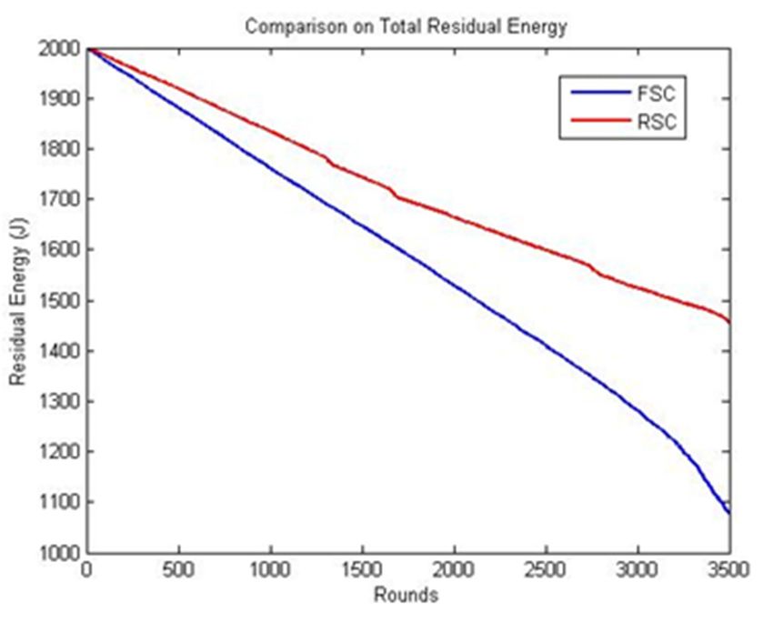
Sensors 2020, 20, 4937                                                                                3 of 15

into k clusters, and nodes join the nearest CH based on the Euclidean distance. However, the periodic
reformation of clusters leads to network overhead.
     Agrawal and Pandey [21] proposed a CH election approach using fuzzy logic. Tentative CHs are
elected in each round based on random numbers. The elected CH then uses two fuzzy parameters,
which are at the local distance and of similar energy level. The local distance is the sum of all distances
from neighboring nodes.
     In a similar approach by Farman et al. [22], the network is partitioned into grids based on the node
location where midpoints are computed using the membership degree. In the approach discussed
by Meng et al. [23], two levels of square shaped grids are used to divide the network into high and
low levels. For intracluster data transmission, a low-level grid is used, and for intercluster data
transmission, a high-level grid is used. However, adopting this technique for large-scale deployment
increases network complexity.
     Moreover, topology construction is also vital for the distribution of nodes uniformly in the clusters
or grids in case of grid-based approaches to make the network efficient. Although the deployment
structure is considered as a grid, forming equal-sized grids in real-time deployment may not be feasible.
Furthermore, the periodic reformation of clusters and the reselection of CHs could significantly increase
energy consumption, thus leading to poor network performance [24–26].
     To achieve reduced power utilization with minimal cost and congestion-aware routing, nodes are
provisioned with transmission range adjustment, to reach the desired receiver. Transmission range
adjustment and multihop forwarding are global positioning system (GPS)-based approaches.
Considering the node’s radio and electrical energy, the combination of Geographic Adaptive Fidelity
(GAF) and DGAF works well [27].
     Lin et al. divided the network area into fan-shaped clusters (FSCs) and placed the sink node at the
center of the fan-shaped coverage [28]. In the FSC, the diameter of the inner circle is twice that of the
outer circle to balance the number of nodes in the cluster. The CH is selected randomly in each circle,
and hierarchical energy level-based routing is followed. The sink node is located in the central area
by default. As random CH selection in each circle increases the transmission distance, frequent CH
selection is required for large-scale deployment. In real-time applications such as smart agriculture and
natural environment protection, it may not be feasible for the sink node to be located in the central area.
     In this paper, the researchers propose an angular inclination-based clustering system to address
the challenges of FSCs, which grabs attention in the high-volume deployment of sensor networks.
This technique divides the high-volume network into virtual circles, and each virtual circle is
further divided into various sectors called clusters to form radial-shaped groups. Moreover, angular
inclination-based clustering has many benefits like minimizing the reclustering rate, ease of use,
and robustness in routing, and accomplishes a balanced network load.

3. Network and Energy Model
     This paper adopted the radio energy model in HEED [10] for free space and multipath channel
models. As the nodes are equipped with quasi-stationary distribution and scattered autonomously in
a network field, the HEED’s energy model is considered to be the most appropriate choice. In addition
to the built-in functionality of sensing nodes, the polar coordinates of each sensing node are known to
that node, and sensing devices are GPS enabled.
     The sensing nodes are generally deployed independently and the distance is measured to connect
the scattered nodes. After the outer structure is defined, the sensing field is divided into virtual circles.
The diameter of the inner layer should be greater than that of the outer layers to avoid the hotspot
issue. The network field is divided by using polar coordinates defined as follows:

•     The radius of the circle (r)
•     The angle (θ)
•     The center position or midpoint of the area (x0 ,y0 )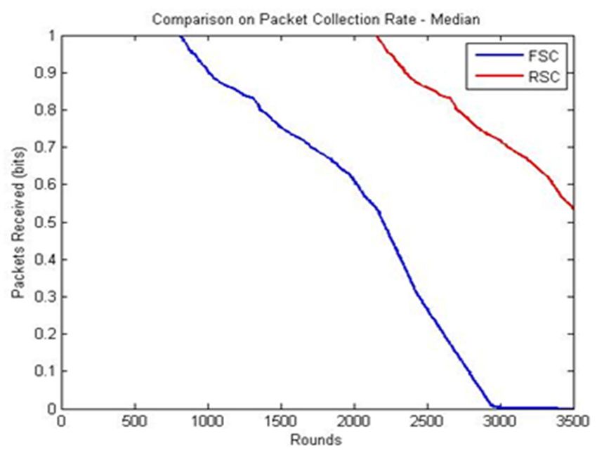
Sensors 2020, 20, 4937                                                                                             4 of 15

Sensors 2020, 20, x FOR PEER REVIEW                                                                               4 of 16
     The sensing field is divided into circular-shaped clusters using polar coordinates of the circle,
whichThe
       uses  the r, θ,
          sensing   field     0 ,y0 ) based
                       andis(xdivided    intooncircular-shaped   clusters using polar coordinates of the circle,
                                                 the following formula:
which uses the , , and ( ˈ, ˈ) based on the following formula:
                                                           angle
                                                     θ=          ∗i                                          (1)
                                                             2
                                                        =        ∗                                          (1)
                                                             2
                                                  x = r ∗ cos(θ) + x0                                        (2)
                                                     = ∗ cos( ) + ˈ                                         (2)
                                                   y = r∗ sin(θ) + y0                                        (3)
                                                     = ∗ sin( ) + ˈ                                         (3)
     The deployment structure design is shown in Figure 1. The diameter of the first layer should be
     The deployment structure design is shown in Figure 1. The diameter of the first layer should be
higher than those of the remaining outer layers. Each segment is further divided into equal-sized
higher than those of the remaining outer layers. Each segment is further divided into equal-sized
groups. Equal-sized groups contain randomly distributed nodes to achieve load balancing. The layers
groups. Equal-sized groups contain randomly distributed nodes to achieve load balancing. The layers
in the area are partitioned into (2∗i − 1) ∗ n groups with n quadrants where i = (1, 2, 3, 4 . . . , m) is the
in the area are partitioned into (2 ∗ i − 1) ∗ groups with n quadrants where = (1,2,3,4 … . ) is
layer from inner to outer structure and n = (2, 4, 6, 8, . . .) represents the number of quadrants the area
the layer from inner to outer structure and = (2,4,6,8, … . ) represents the number of quadrants the
gets partitioned.
area gets partitioned.

                           Figure 1. Deployment structure of radial-shaped clustering.
                         Figure 1. Deployment structure of radial-shaped clustering.
      Since the network field is portioned into concentric rings in fan shaped clustering by Lin et al. [28],
      Since the network field is portioned into concentric rings in fan shaped clustering by Lin et al.
the same layering and quadrants approach is adopted in this work. The quadrants are applied from 2
[28], the same layering and quadrants approach is adopted in this work. The quadrants are applied
to 8 and dynamically changing the quadrant is beyond the scope of this paper. The Euclidean distance
from 2 to 8 and dynamically changing the quadrant is beyond the scope of this paper. The Euclidean
is used in HEED and applied to calculate energy requirements within the cluster region, and also the
distance is used in HEED and applied to calculate energy requirements within the cluster region, and
energy requirements for intercluster communication.
also the energy requirements for intercluster communication.
4. Radial-Shaped Geo Clustering and Angular Routing
4. Radial-Shaped Geo Clustering and Angular Routing
      The sensing nodes are deployed randomly over the deployment area, and the network area is divided
into aThe  sensing nodes
       circular-shaped         are deployed
                         virtual    concentric randomly
                                                  m number over    the Moreover,
                                                             of rings.  deployment     area,
                                                                                    each     andring
                                                                                         virtual  the has
                                                                                                      network     area of
                                                                                                           k number     is
divided   into a circular-shaped        virtual  concentric      number    of rings. Moreover,   each  virtual
clusters. The sectors of radial-shaped virtual concentric rings θ are calculated from the midpoint of the       ring  has
   number
network      of plot
          area  clusters.  The
                     (xCenter     sectors
                              , yCenter ) to of
                                             theradial-shaped
                                                 radius of eachvirtual   concentric
                                                                 ring based          ringsand
                                                                              on the sine   θ are calculated
                                                                                               cosine          from the
                                                                                                      transformations
midpoint
as given inofalgorithm
               the network
                         linesarea1 to 4. The ( nodes, are deployed
                                                              ) to therandomly
                                                                         radius ofand
                                                                                    eacheach
                                                                                          ringnode
                                                                                               based  on the sine
                                                                                                    identifies        and
                                                                                                                its polar
cosine  transformations      as  given    in algorithm  lines 1 to  4. The nodes   are deployed
coordinates in line no. 8. The node identifies its own sector from lines 9 to 16 in Algorithm 1.  randomly    and    each
node identifies its polar coordinates in line no. 8. The node identifies its own sector from lines 9 to 16
in Algorithm 1.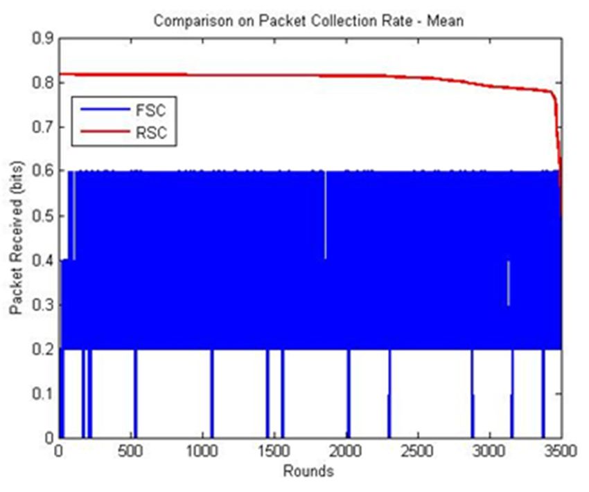
Sensors 2020, 20, 4937                                                                                  5 of 15

 Algorithm 1. Radial-shaped clustering (RSC).

 1:     Input: r, m, (xCenter , yCenter )
 2:     Output: Total number of clusters
 3:     k = (2∗ i − 1) ∗ n
 4:     for i = 1 to k
 5:           for j = 1 to i
 6:             Generate the number of sectors according to the Equations (1)–(3)
 7:             plot(x, y)
 8:           end for
 9:     end for

 10:    Deploy the nodes randomly and measure the polar coordinates by using the formula r = sqrt x2 + y2
                y
        θ = atan x
 11:    for i = 1 to s.no
 12:    if nodelayer(i) == r
 13:            k = (2 ∗ i − 1) ∗ n
 14:                      for j = 1 to k_nodes
 15:                                   if node(i)angle ≤ sector(i)angle
 16:                                node(i).positionsector(i).position
 17:                                  end if
 18:                      end for
 19:          end if
 20:    end for

4.1. CH Selection in RSC
      The clusters are partitioned in each sector of the radial-shaped virtual ring, and the nodes identify
their position. For each cluster, a Euclidean distance is calculated for all the intracluster nodes as local
coordinates, and the node closest to the midpoint of a cluster becomes the initial CH. Subsequently,
the re-election process starts whenever the CH’s battery level is less than the set threshold. The sensing
node with the highest battery level becomes the CH of the cluster.
      The procedure to select the CH is presented in Algorithm 2. The size of randomly deployed nodes
Size (A), midpoints Size (Grp), side length of a cluster (a) and the radius (r) are taken as the input
parameters. From the lines 1 to 4 in the Algorithm 2, the midpoint of the sector is taken as the minimum
threshold value and calculates the x, y coordinates for each node to compare with the maximum of x,
y coordinates in each sector. The lines Nos. 6 to 12 measure the radius, the angle and the distance of
each node within the sector. The node which is nearest to the midpoint with maximum energy is taken
as a CH in each sector according to the lines Nos. 15 to 19 in Algorithm 2. This procedure continues
until all the CHs are selected in the deployment area.
      The CH sends data towards the next lower layer of the ring, which in turn sends the data to the next
lower layer and so on. This action terminates when the sink node receives the data. The CH may also
act as the relay node. In this strategy, the CH is assumed to be simple and efficient, which minimizes
the intracluster communication and reclustering costs of the repetition process.
      Furthermore, the CH broadcasts its head message to all the other members of the clusters. First,
it reduces the intracluster communication cost as the CH is located at the midpoint of the clusters.
Second, the reclustering frequency is minimized as it happens only when no node is available in the
midpoint of the cluster area.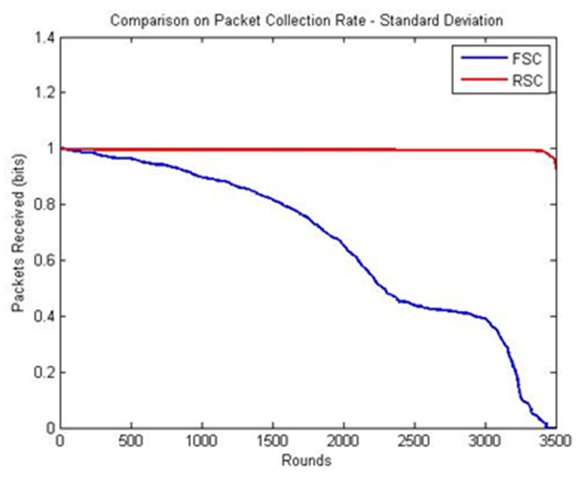
Sensors 2020, 20, 4937                                                                            6 of 15

 Algorithm 2. CH selection in radial-shaped clusters.

 1:     Input: size(A), size(grp), a, r
 2:     Output: Each cluster with CH
 3:     for i = 1 to Size(Grp)
 4:           Find the min. and max. of x, y coordinates for each sector with a
 5:           k=1
 6:           for j = 1 to Size(A)
 7:             if min(x) ≤ node.x ≤ max(x) and min( y) ≤ node.y ≤ max( y)
 8:                   Ck (i) := node.id
 9:                  radiusCk = r/2
 10:                 angle(Ck (i)) = θ/2
 11:                 Disti ( j) = the distance between the node location
 12:                 end if
 13:          end for
 14:    end for
 15:    for l = 1 to node_count do
 16:                 Mini (l) = min(Disti (l))
 17:            if (Mini (l) == Mini (l − 1))
 18:                            Verify the level of energy and select the node with max. energy
        Chi (k) = Minl (node.id)
 19:            end if
 20:          k=k+1
 21:    end for

4.2. Routing Model
     In RSC, intracluster communication is established with single-hop routing. For intercluster
communication, multihop or hierarchical routing is necessary, because the data from a cluster
aggregated by the CH are transmitted to the sink node via other CHs in the structure deployed
nearby. The sink node can be located anywhere within the network deployment, and the routing
path is established based on the location of the sink node. Data transmission is a suboptimal process
using traditional routing models based on the shortest path distance. We adopted chain-based
routing to achieve optimal data transmission. Therefore, we propose a routing algorithm based on
the angular inclination technique used in Lalitha et al. [17] mainly to transmit data toward the sink
node. The primary objective is to identify an optimal routing path from every CH to the sink node,
as implemented in [23,27–29].
     To find the optimal path, a threshold angle is taken and the angle between the CH and the sink is
calculated by finding the angular difference from lines Nos. 3 to 6 in Algorithm 3. Once the angle is
measured, the distance between inter-CHs towards the sink is calculated from lines 7 to 11. Initially,
neighbor CH is zero. After the distance and the angular measurement, the CH with minimum distance
and maximum energy is selected as a next hop CH. This process is depicted in the algorithm from lines
17 to 23.
     In this angular routing, an angular structure is formed between two CHs, and the data are
forwarded from one angular aligned CH to the other. It reduces the hop count, unlike the heuristic
approach of finding the shortest path. Data forwarded from CH to CH are random in the LEACH
protocol, and the chain model-based forwarding of data from one cluster member to another is
implemented in PEGASIS. There is no assurance of reaching the sink node in the former technique
and finding alternate routes is complex in the case of node failure in the latter. These problems are
alleviated in the current routing technique that is applied in RSC.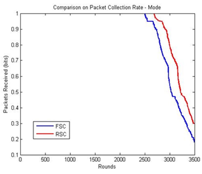
Sensors 2020, 20, 4937                                                                          7 of 15

 Algorithm 3. Angular Routing in RSC.

 1:     Input: α- Threshold value, CHn –number of CHs
 2:     Output: Optimal routing path to the Sink
 3:     Find the angle amongst CH and the Sink
 4:     for Ch(i) =1 to CHn
                        y
 5:         θ = tan−1 x
 6:          β1 = θ + α        β2 = θ − α
 7:          for Ch(i) =1 to l
 8:             if Ch(i) ! = Ch(l)
 9:                     if Ch(l) .degree ≥ β2 &&Ch(l) .degree < β1

 10:                                    path Ch(i) = l

 11:                                    distance ch(i) = Dist(ch(i) , ch(l) )
 12:                               end if
 13:                   end if
 14:         end for
 15:    end for
 16:    Neighbor( Ch(i) )=0

 17:    for j=1 to path Ch(i)

 18:         if path ch(i) , ch( j) ! = 0
 19:                   (Mini ( j) == Mini ( j − 1))
 20:                                  Find the node which has min.              distance
        Mindst (node.id) = Chi ( j)
 21:                     end if
 22:    end for
 23:    nexthop(ch(i) ) = Mindst (node.id)

5. Simulation and Performance Evaluation
     The RSC algorithm was implemented using MATLAB 2013a and core i5 processor with Windows-7.
The transmission radius of the sensor nodes was at 100 m.
     The experiment results were taken from twenty different scenarios like varying the number of
nodes from 500 to 1000. The network field was assumed to be a virtual circular-shaped area where
sensor nodes were distributed randomly. The number of nodes deployed and the number of rounds
were changed frequently to obtain the cluster data for further analysis. The sink node was placed
in the center of the circular area initially. The sink node location was changed randomly in different
scenarios. The parameters used in MATLAB are defined in Table 1.
     The cluster head selection in RSC is presented as an example scenario in Figure 2. The radius
of the inner circle was twice that of the remaining circles to avoid the hotspot issue since all the
communications were towards the sink location. The angle θ was taken as 90◦ for fixing the quadrant
in this example scenario, hence n was 4 and each quadrant was taken as a single sector. Subsequently,
the second layer was subdivided into three sectors by π3 . Furthermore, the next layer was subdivided
into five sectors by π5 for the third circle, and so on. The nodes were thrown randomly in the
deployment area and each sector was considered as a cluster. Each cluster needed a CH to aggregate
the data.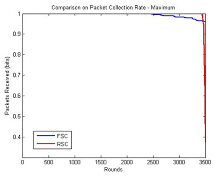
50 nJ/bit
10 pJ / bits /m2)
0.0013 pJ / bits / m4)
5 nJ / (bit ∗ signal)
Sensors 2020, 20, 4937 8 of 15
√
Table 1. Simulation parameters used in RSC.
x,y coordinates of midpoint of grid ( , )
x,y coordinatesParameters Used
of all nodes ( , ) Values
Area of deployment (x,y) 500 m ∗ 500 m
Number of rounds 500
Number of nodes 1000
Control packet
Coordinate sizesink node (Sx , S y)
of the 200
(260,bits
260) m
The initial
Data packet size energy of each sensor 2 J (Joule)
3000 bits
Eelec 50 nJ/bit
εfs 10 pJ/bits/m2 )
The cluster head
εmp selection in RSC is presented as an example 0.0013scenario
pJ/bits/min
4 ) Figure 2. The radius of
the inner circle was
EDA twice that of the remaining circles to5 avoid nJ/(bit ∗the hotspot issue since all the
signal)
√ fs
communications were
d0 towards the sink location. The angle θ was taken
εmp
as 90˚ for fixing the quadrant
in this example x,yscenario,
coordinates hence wasof4grid
of midpoint and each quadrant
S px , p y was taken as a single sector.
Subsequently, thex,y coordinates
second layer of all nodes
was A(x, y)by . Furthermore, the next layer
subdivided into three sectors
Number of rounds K 500
was subdivided into five sectors by for the third circle, and so on. The nodes were thrown
Control packet size Pctrl 200 bits
randomly in the deployment
Data packet size area and each sector was considered
Pdata 3000 bitsas a cluster. Each cluster needed a
CH to aggregate the data.
Figure
Figure 2. Node
2. Node deployment
deployment andand
CHCH selection.
selection.
The CH was identified by the minimum distance closest to the midpoint of the cluster, as shown
The CH was identified by the minimum distance closest to the midpoint of the cluster, as shown
in Lalitha et al. [17,18]. Initially, the sink was located at the center of the network field, and then it was
in Lalitha et al. [17,18]. Initially, the sink was located at the center of the network field, and then it
changed dynamically to evaluate the performance.
was changed dynamically to evaluate the performance.
The process of routing takes place when the node forwards the data collected towards its CH.
The probability of data transmitting to the nearest CH towards the sink node is a binomial polynomial
problem. Angular inclination routing is one of the alternatives to ensure that the data can be reached
to the Sink node.
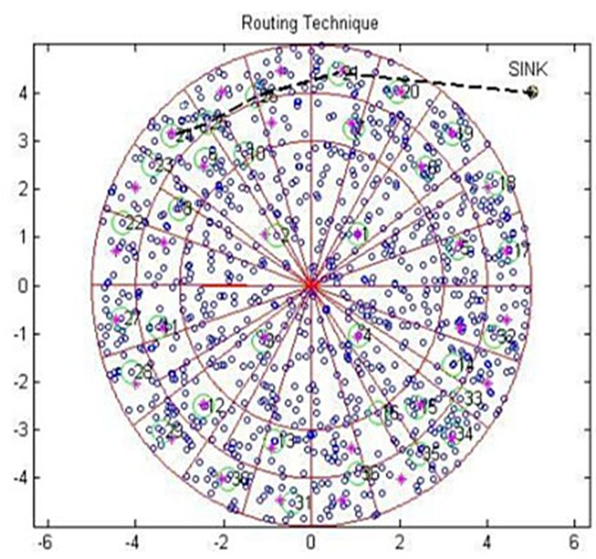
The CH transmitted the data towards the subsequent lower layer sensing node in the angular
inclination routing, as discussed in [23,30]. This process continued toward the angle of the sink node
until the data reached the sink node. The scenario presented in Figure 3 shows that the third layer of
the CH wanted to transmit the data to the sink. The sink location was identified and a virtual path was
framed from CH to the sink with 30-degree angular inclination. In this routing, the number of hops
was greatly reduced and there was a moderate increase in the transmission range.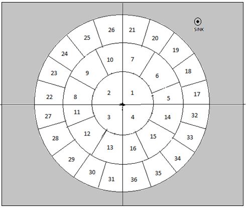
The CH transmitted the data towards the subsequent lower layer sensing node in the angular
inclination routing, as discussed in [23,30]. This process continued toward the angle of the sink node
until the data reached the sink node. The scenario presented in Figure 3 shows that the third layer of
the CH wanted to transmit the data to the sink. The sink location was identified and a virtual path
was  framed
Sensors 2020, 20,from
                  4937 CH to the sink with 30-degree angular inclination. In this routing, the number
                                                                                                   9 ofof
                                                                                                       15
hops was greatly reduced and there was a moderate increase in the transmission range.

                                           Figure 3. Routing for the RSC.
                                        Figure 3. Routing for the RSC.
 5.1. Behavioral Analysis of the RSC
5.1. Behavioral Analysis of the RSC
      The performance of the RSC was analyzed based on the following criteria: the number of live
      The
 nodes,    performance
         the total networkof residual
                             the RSCenergy,
                                          was analyzed
                                                  and thebased
                                                             packeton   the following
                                                                     received     ratio. criteria: the number of live
nodes, the total network residual energy, and the packet received ratio.
1. LiveLivesensing
             sensing nodes:
                      nodes: thethetotal
                                     total numbers
                                           numbersof   of sensing
                                                           sensing nodes
                                                                    nodes withwith anan energy
                                                                                        energy level
                                                                                                level greater
                                                                                                      greater than
                                                                                                               than the
                                                                                                                    the
       thresholdare
      threshold   arecalled
                      calledlive
                              livesensing
                                    sensingnodes.
                                              nodes.
2.
 2. Total
       Total residual
              residual energy: this
                                  this is the total
                                              total energy
                                                     energylevel
                                                              levelofofall
                                                                        alllive
                                                                             livesensing
                                                                                   sensingnodes
                                                                                           nodes   measured
                                                                                                 measured  in in joules
                                                                                                              joules (J).
 3. (J).
       Packet received ratio: the packet received ratio for each round is calculated as the ratio of the
3. Packet      received
       total number      ratio: the
                      of packets      packet and
                                   received    received    ratiocount.
                                                    the node     for each round is calculated as the ratio of the
      total number of packets received and the node count.
      The packet received ratio metric used statistical measures as referred to in Chen [31], are listed below:
      The packet received ratio metric used statistical measures as referred to in Chen [31], are listed
 • below:
      Mean
••    Median
      Mean
•• Median
      Mode
••    Maximum
      Mode
•• Maximum
      Variance or standard deviation
•     Variance or standard deviation
      Figure 4 shows the number of live nodes, the residual power level of all the nodes, and the ratio
of packets
      Figurecollected
             4 shows thebased  on the
                            number   oftime   (number
                                        live nodes,  theof rounds).
                                                         residual powerAs shown
                                                                           level ofinallFigure  4a, the
                                                                                          the nodes,    number
                                                                                                      and        of
                                                                                                          the ratio
live  nodes  decreased   as  the number    of  rounds  increased.   It was   observed     that all the
of packets collected based on the time (number of rounds). As shown in Figure 4a, the number of live   nodes  were
alive until
nodes        700 s and
        decreased        started
                    as the  numberto die  at about
                                      of rounds     1700 s. The
                                                  increased.      energy
                                                             It was         levelthat
                                                                      observed    indicated
                                                                                         all thethat thewere
                                                                                                 nodes   proposed
                                                                                                              alive
algorithm
until       achieved
      700 s and  startedimproved    load balancing.
                          to die at about  1700 s. TheAs   shown
                                                        energy     in Figure
                                                                level          4b,that
                                                                       indicated    the the
                                                                                          residual  power
                                                                                              proposed     level of
                                                                                                        algorithm
the total deployed nodes decreased with the increase in duration. The sudden increase in energy
consumption of a network was caused by the following: first, the nodes’ count expired after certain
duration; the long route needed to be identified by the packets to reach the sink node. Secondly,
the frequent re-election process. The energy level was expended rapidly in both cases. Figure 4c shows
that the rate of packets received started to decrease at the duration of 700 s. It was observed that up to
700 s, the packet collection rate was 100% and then it decreased subsequently. Even after 2000 s, almost
50% of the nodes were still alive, which gave a packet collection rate of 50%. This indicated that the
nodes were alive in the first layer and showed that the RSC achieved load balancing.
long route needed to be identified by the packets to reach the sink node. Secondly, the frequent re-
election process. The energy level was expended rapidly in both cases. Figure 4c shows that the rate
of packets received started to decrease at the duration of 700 s. It was observed that up to 700 s, the
packet collection rate was 100% and then it decreased subsequently. Even after 2000 s, almost 50% of
the nodes were still alive, which gave a packet collection rate of 50%. This indicated that the 10
Sensors 2020, 20, 4937
nodes
of 15
were alive in the first layer and showed that the RSC achieved load balancing.
(a) (b)
(c)
Figure 4.
Figure 4. Behavioral
Behavioralanalysis
analysisofofRSC:
RSC:(a)(a)
thethe number
number of live
of live nodes;
nodes; (b) residual
(b) the the residual power
power level level of
of RSC;
RSC; and (c) the packet received ratio
and (c) the packet received ratio of RSC. of RSC.
5.2.
5.2. Comparison
Comparison of
of RSC
RSC with
with Fan-Shaped
Fan-Shaped Clustering
Clustering
The
TheRSCRSCresults
resultswere compared
were comparedagainst the existing
against FSC in Lin
the existing FSCetinal. Lin
[28] to
et analyze
al. [28]theto performance
analyze the
of
performance of RSC since both the algorithms applied angular clustering and aimed toefficiency
RSC since both the algorithms applied angular clustering and aimed to increase energy increase
and to reduce
energy reclustering
efficiency costs in
and to reduce large-scalecosts
reclustering networks.
in large-scale networks.
The
The existing
existing algorithm
algorithm FSCFSC was
was compared
compared with
with HEED
HEED to to find
find the
the number
number of of alive
alive nodes
nodes with
with
2000
2000 rounds, i.e., 2000 seconds and produced the results as 42% live nodes with more than 40%
rounds, i.e., 2000 seconds and produced the results as 42% live nodes with more than 40% live
live
nodes
nodesleft
leftininFSC
FSCcompared
compared to 1/3 of nodes
to 1/3 withwith
of nodes 10% 10%
energy in HEED.
energy Since the
in HEED. existing
Since work is work
the existing alreadyis
compared with the state-of-the-art algorithm, FSC alone was taken for comparison
already compared with the state-of-the-art algorithm, FSC alone was taken for comparison and and simulation.
Both RSC and
simulation. FSC
Both were
RSC executed
and FSC wereup executed
to 3500 rounds.
up to 3500 rounds.
Similarly,
Similarly, the existing work was comparedwith
the existing work was compared with HEED
HEED forfor the
the evaluation
evaluation of of total
total residual
residual energy
energy
and packet collection rate. In most of the scenarios, it was executed up to 2000
and packet collection rate. In most of the scenarios, it was executed up to 2000 rounds. rounds. To achieve better
To achieve
results with long duration and large-scale network, the FSC was compared with RSC for 3500 rounds
for the above two parameters.
The results of RSC and FSC were analyzed based on the total live nodes. Initially, the number of
nodes was stable in both the cases. In FSC, the number of nodes started to decrease at 1800 rounds and
reaches 860 at 3500 rounds. Conversely, in RSC, the number of nodes started to decrease at 2800 rounds
and reached 920 at 3500 rounds. This indicated that the nodes started consuming energy evenly; they
died at almost the same time. Figure 5a shows considerable load balancing up to 3000 rounds. The total
residual energy decreased with time, as shown in Figure 5b, as the node had to find a route to reachrounds for the above two parameters.
The results of RSC and FSC were analyzed based on the total live nodes. Initially, the number of
nodes was stable in both the cases. In FSC, the number of nodes started to decrease at 1800 rounds
and reaches 860 at 3500 rounds. Conversely, in RSC, the number of nodes started to decrease at 2800
rounds and reached 920 at 3500 rounds. This indicated that the nodes started consuming energy
Sensors 2020, 20, 4937 11 of 15
evenly; they died at almost the same time. Figure 5a shows considerable load balancing up to 3000
rounds. The total residual energy decreased with time, as shown in Figure 5b, as the node had to find
a route
the to reach
sink node andthe
the sink node and
reclustering the reclustering
process. process.
RSC performed RSC
better performed
because better because
the transmission the
distance
transmission
was less than distance was less than that in FSC.
that in FSC.
(a) (b)
Figure 5. Comparison of RSC and FSC: (a) the number of live nodes and (b)
(b) the
the total
total residual
residual energy.
energy.
The packet received ratio is considered as the most significant measure because it reveals packet
loss and the dead nodes in the network.
network. Packet loss may occur when
1.
1. none
none of
of the
the nodes
nodes is
is selected
selected asas the
the CH,
CH,
2.
2. the
the CH node could not find the forwarder to
CH node could not find the forwarder to reach the sink
reach the sink node,
node, and
and
3. the distance to reach the relay node is much greater.
3. the distance to reach the relay node is much greater.
The packet received ratio was analyzed using statistical measures considering the factors
The packet
mentioned abovereceived
and theratio wasscale
large analyzed using
of the statistical measures
applications considering
[29,32–39]. the factors
For example, mentioned
the mean values
above and the large scale of the applications [29,32–39]. For example, the mean values were considered
were considered effective for real-time traffic applications, but event-based applications would prefer
effective for real-time
median and trafficSome
mode values. applications, but event-based
of the applications applications
and preferred wouldmeasures
statistical prefer median
were asand mode
follows:
values. Some of the applications and preferred statistical measures were as follows:
• Mean—power distribution units
•• Mean—power
Median—capacity distribution
planningunits
or cost predictions
•• Median—capacity planning or
Mode—power consumption ofcost predictions
an entire network operation center
•• Mode—power
Maximum—domesticconsumption of an entire transfer
applications/heat network operation center
•• Standard deviation and/or
Maximum—domestic variance—to
applications/heat trigger a warning or an alarm if a system operates
transfer
• outside an acceptable range
Standard deviation and/or variance—to trigger a warning or an alarm if a system operates outside
an
Theacceptable range ratio comparison of the FSC and RSC is shown in Figure 6. In FSC, the
packet received
packets
Thereceived were 0.6,
packet received whereas
ratio in RSC,
comparison of the
the packets
FSC andreceived were 0.82,
RSC is shown and 6.
in Figure it started
In FSC, to
thedecrease
packets
gradually to 0.8 at 2700 rounds and reached 0.5 at 3500 rounds based on the mean values.
received were 0.6, whereas in RSC, the packets received were 0.82, and it started to decrease gradually This is
because the radius of the inner and outer layers is equal for RSC, but FSC produces
to 0.8 at 2700 rounds and reached 0.5 at 3500 rounds based on the mean values. This is because an inner layer
the
that is twice that of the outer layer, which increases the transmission distance. The uniform
radius of the inner and outer layers is equal for RSC, but FSC produces an inner layer that is twice that size of
the layers in RSC constitutes a high mean and median packet collection rate, as shown
of the outer layer, which increases the transmission distance. The uniform size of the layers in RSCin Figure 6a.
constitutes a high mean and median packet collection rate, as shown in Figure 6a.
RSC and FSC produced results with slight deviations in the mode and maximum statistical
measures. Both the algorithms aim to reduce the frequency of the reclustering cost, which was achieved
at 2700 rounds in the FSC and 3000 rounds in RSC, as shown in Figure 6c,d. Subsequently, the packet
collection rate decreased rapidly due to the finding of the relay node and transmission distance with
the present live nodes.Sensors 2020, 20, 4937 12 of 15
Sensors 2020, 20, x FOR PEER REVIEW 12 of 16
(a) (b)
(c) (d)
(e)
Figure
Figure 6.
6. Comparison
Comparisonofofthe
the package
packagecollection
collectionrate:
rate:(a)
(a)mean;
mean;(b)
(b)median;
median;(c)
(c)mode;
mode;(d)
(d)maximum;
maximum;
and (e) standard deviation.
and (e) standard deviation.
The results
RSC and FSC of produced
RSC and FSC in standard
results deviation
with slight showed
deviations thatmode
in the the size
andofmaximum
a data set statistical
may vary
according to
measures. the the
Both timealgorithms
and range. aimIn a to
certain interval
reduce period between
the frequency of thetwo grouping practices,
reclustering cost, whichthewas
rate
of packet collection reduces because of the nonexistence of CHs. If the variance
achieved at 2700 rounds in the FSC and 3000 rounds in RSC, as shown in Figure 6c,d. Subsequently, measure is high,
the packet
the deviation of data israte
collection alsodecreased
high, which leads due
rapidly to inadequate analysis.
to the finding This
of the is identified
relay node and in transmission
FSC owing to
the size of
distance thethe
with central area.live
present Data are transmitted from the outer layer to the inner layer until they reach
nodes.
the CH
Thewhich
resultsisoflocated
RSC and in the
FSCcentral area. Frequent
in standard deviationdata collection
showed that theleads
sizetoofrepeated reclustering,
a data set may vary
according to the time and range. In a certain interval period between two grouping practices, the rate
of packet collection reduces because of the nonexistence of CHs. If the variance measure is high, theSensors 2020, 20, 4937 13 of 15
which decreases the packet collection rate. In the FSC, the initial packet received started decreasing
gradually from the starting round and reached 0 at 3500 rounds, whereas in RSC, the initial packet
received was 1.00, and it started to decrease gradually at 3400 rounds and reached 0. 85 at about
3500 rounds.
Figure 6e shows that the proposed system maintained its stability and achieved an improved
packet collection rate compared with the existing system. This work tries to reveal that compared to
the existing application-oriented algorithms [30,31,39–44], RSC performs better in the event-based and
time-critical applications.
The scenarios and the number of rounds used for evaluating the performance of RSC was inherited
from fan-shaped clustering and the only difference is both the algorithms were implemented and
evaluated for different statistical measures [35–41].
Since RSC and FSC were evaluated with same set of scenarios, the improvement in percentage
may be addressed stochastically. But the improvement varies according to the parameter selected for
comparison. Here, the number of nodes alive are 16% more in RSC and from the energy conservation
point of view, RSC produces a 34% improvement, whereas, RSC produces 45% improvement in
statistical measures mean and median. All the above results are obtained when compared with
FSC. Hence, the results were not addressed stochastically. In future, this might be addressed with
various quadrants.
6. Conclusions and Future Scope
This paper proposes angular inclination-based RSC and routing. The network area is considered
as a circular area, and it is divided into equal-sized virtual concentric rings based on the radius of the
circle. Each ring is further divided into equal-sized clusters, which increases gradually from the inner
layer to the outer layer. The CH is selected based on the nearest distance to the midpoint of the cluster.
Furthermore, the CH is updated based on the number of live nodes and the residual energy to ensure
load balancing. The number of nodes and packet collection rates are high because RSC is implemented
for large-scale networks. To identify the optimal aggregation measures for large-scale applications,
the statistical measures are considered with the objective of a high packet collection rate with reduced
reclustering frequency. There is a tradeoff between the transmission distance and the range when the
quantity of live nodes and routing is considered. It was found that the RSC outperformed the existing
FSC in network energy conservation.
Even though the present work yielded better results compared to the existing state-of-the-art
algorithms, static random deployment with the manual change of quadrants is to be implemented in
future. For real-time applications, it would be more useful if the quadrant is changed dynamically.
This work addresses only flat surface deployment. In future, it should be extended to address regions
with sloppy surfaces to bring realistic results. In addition to this, security of sensor networks and
secure data transmission has to be taken into consideration for further improvement.
Author Contributions: Conceptualization, L.K., R.K.D. and D.G.G.; methodology, L.K., D.G.G. and T.R.G.;
software, R.K.D., T.R.G.; validation, L.K., R.K.D. and D.G.G.; investigation, L.K., R.K.D. and D.G.G.; resources,
T.R.G., M.K.A., and E.A.N.; data curation, M.K.A., L.K.; writing—original draft preparation, L.K., R.K.D. and
D.G.G.; writing—review and editing, M.K.A., T.R.G. and E.A.N.; project administration, D.G.G., T.R.G. and
E.A.N.; funding acquisition, M.K.A. and E.A.N. All authors have read and agreed to the published version of
the manuscript.
Funding: The authors extend their appreciation to King Saud University for funding this work through Researchers
supporting project number (RSP-2020/164), King Saud University, Riyadh, Saudi Arabia.
Acknowledgments: The authors extend their appreciation to King Saud University for funding this work through
Researchers supporting project number (RSP-2020/164), King Saud University, Riyadh, Saudi Arabia.
Conflicts of Interest: The authors declare no conflict of interest.Sensors 2020, 20, 4937 14 of 15
References
1. Numan, M.; Subhan, F.; Khan, W.Z.; Hakak, S.; Haider, S.; Reddy, G.T.; Jolfaei, A.; Alazab, M. A
Systematic Review on Clone Node Detection in Static Wireless Sensor Networks. IEEE Access 2020, 8,
65450–65461. [CrossRef]
2. Pandita, D.; Malik, R.K. A Survey on Clustered and Energy Efficient Routing Protocols for Wireless Sensor
Networks. Int. J. Trend Sci. Res. Dev. 2018, 2, 1026–1030. [CrossRef]
3. Kumar, A.; Shwe, H.Y.; Wong, K.J.; Chong, P.H.J. Location-based routing protocols for wireless sensor
networks: A survey. Wirel. Sens. Netw. 2017, 9, 25–72. [CrossRef]
4. Kardi, A.; Zagrouba, R. RaCH: A New Radial Cluster Head Selection Algorithm for Wireless Sensor Networks.
Wirel. Pers. Commun. 2020, in press. [CrossRef]
5. Farouk, F.; Rizk, R.; Zaki, F.W. Multi-level stable and energy-efficient clustering protocol in heterogeneous
wireless sensor networks. IET Wirel. Sens. Syst. 2014, 4, 159–169. [CrossRef]
6. Iwendi, C.; Maddikunta, P.K.R.; Gadekallu, T.R.; Lakshmanna, K.; Bashir, A.K.; Piran, M.J. A metaheuristic
optimization approach for energy efficiency in the IoT networks. Softw. Pract. Exp. 2020, in press. [CrossRef]
7. Patel, H.; Singh Rajput, D.; Thippa Reddy, G.; Iwendi, C.; Kashif Bashir, A.; Jo, O. A review on classification
of imbalanced data for wireless sensor networks. Int. J. Distrib. Sens. Netw. 2020, 16, 1550147720916404.
[CrossRef]
8. Pintea, C.-M.; Pop, P.C.; Zelina, I. Denial jamming attacks on wireless sensor network using sensitive agents.
Logic J. IGPL 2015, 24, 92–103. [CrossRef]
9. Batra, P.K.; Kant, K. LEACH-MAC: A new cluster head selection algorithm for Wireless Sensor Networks.
Wirel. Netw. 2016, 22, 49–60. [CrossRef]
10. Younis, O.; Fahmy, S. HEED: A hybrid, energy-efficient, distributed clustering approach for ad hoc sensor
networks. IEEE Trans. Mobile Comput. 2004, 3, 366–379. [CrossRef]
11. Maddikunta, P.K.R.; Gadekallu, T.R.; Kaluri, R.; Srivastava, G.; Parizi, R.M.; Khan, M.S. Green communication
in IoT networks using a hybrid optimization algorithm. Comput. Commun. 2020, 159, 97–107. [CrossRef]
12. Sawarna Priya, R.M.; Bhattacharya, S.; Maddikunta, P.K.R.; Somayaji, S.R.K.; Lakshmanna, K.; Kaluri, R.;
Hussien, A.; Gadekallu, T.R. Load balancing of energy cloud using wind driven and firefly algorithms in
internet of everything. J. Parallel Distrib. Comput. 2020, 142, 16–26. [CrossRef]
13. Hsiao, H.; Su, H. On Optimizing Overlay Topologies for Search in Unstructured Peer-to-Peer Networks.
IEEE Trans. Parallel Distrib. Syst. 2012, 23, 924–935. [CrossRef]
14. Akl, R.; Kadiyala, P.; Haidar, M. Nonuniform Grid-Based Coordinated Routing in Wireless Sensor Networks.
J. Sens. 2009, 2009, 491349. [CrossRef]
15. Ma, J.; Wang, S.; Meng, C.; Ge, Y.; Du, J. Hybrid energy-efficient APTEEN protocol based on ant colony
algorithm in wireless sensor network. EURASIP J. Wirel. Commun. Netw. 2018, 2018, 102. [CrossRef]
16. Liu, X. Atypical Hierarchical Routing Protocols for Wireless Sensor Networks: A Review. IEEE Sens. J. 2015,
15, 5372–5383. [CrossRef]
17. Lalitha, K.; Thangarajan, R.; Udgata, S.K.; Poongodi, C.; Sahu, A.P. GCCR: An Efficient Grid Based Clustering
and Combinational Routing in Wireless Sensor Networks. Wirel. Pers. Commun. 2017, 97, 1075–1095.
[CrossRef]
18. Lalitha, K.; Thangarajan, R.; Poongodi, C.; Anand, D.V. Sink Originated Unique Algorithm for Clustering
and Routing to forward Aggregated Data in Wireless Sensor Networks. In Proceedings of the 2018
International Conference on Intelligent Computing and Communication for Smart World (I2C2SW), Erode,
India, 14–15 December 2018; pp. 127–130.
19. Mahajan, S.; Malhotra, J.; Sharma, S. Energy Balanced Heuristic Approach for Path Selection Using Graph
Theory. Procedia Comput. Sci. 2015, 46, 101–108. [CrossRef]
20. Ray, A.; De, D. Energy efficient clustering protocol based on K-means (EECPK-means)-midpoint algorithm
for enhanced network lifetime in wireless sensor network. IET Wirel. Sens. Syst. 2016, 6, 181–191. [CrossRef]
21. Agrawal, D.; Pandey, S. Optimization of the selection of cluster-head using fuzzy logic and harmony search
in wireless sensor networks. Int. J. Commun. Syst. 2020, e4391, in press. [CrossRef]
22. Farman, H.; Javed, H.; Ahmad, J.; Jan, B.; Zeeshan, M. Grid-Based Hybrid Network Deployment Approach
for Energy Efficient Wireless Sensor Networks. J. Sens. 2016, 2016, 2326917. [CrossRef]Sensors 2020, 20, 4937 15 of 15
23. Meng, X.; Shi, X.; Wang, Z.; Wu, S.; Li, C. A grid-based reliable routing protocol for wireless sensor networks
with randomly distributed clusters. Ad Hoc Netw. 2016, 51, 47–61. [CrossRef]
24. Tian, Y.; Tang, Z.; Yu, Y. Energy-balanced adaptive clustering routing for indoor wireless sensor networks.
J. Electron. Inf. Technol. 2014, 35, 2992–2998. [CrossRef]
25. Merzoug, M.A.; Boukerche, A.; Mostefaoui, A.; Chouali, S. Spreading Aggregation: A distributed collision-free
approach for data aggregation in large-scale wireless sensor networks. J. Parallel Distrib. Comput. 2019, 125,
121–134. [CrossRef]
26. Ebadi, S. A Multihop Clustering Algorithm for Energy Saving in Wireless Sensor Networks. ISRN Sens. Netw.
2012, 2012, 817895. [CrossRef]
27. Soni, V.; Mallick, D.K. A Novel Scheme to Minimize Hop Count for GAF in Wireless Sensor Networks:
Two-Level GAF. J. Comput. Netw. Commun. 2015, 2015, 527594. [CrossRef]
28. Lin, H.; Wang, L.; Kong, R. Energy Efficient Clustering Protocol for Large-Scale Sensor Networks. IEEE Sens. J.
2015, 15, 7150–7160. [CrossRef]
29. Karakus, C.; Gurbuz, A.C.; Tavli, B. Analysis of Energy Efficiency of Compressive Sensing in Wireless Sensor
Networks. IEEE Sens. J. 2013, 13, 1999–2008. [CrossRef]
30. Han, Z.; Wu, J.; Zhang, J.; Liu, L.; Tian, K. A General Self-Organized Tree-Based Energy-Balance Routing
Protocol for Wireless Sensor Network. IEEE Trans. Nucl. Sci. 2014, 61, 732–740. [CrossRef]
31. Chen, G.; Li, C.; Ye, M.; Wu, J. An unequal cluster-based routing protocol in wireless sensor networks.
Wirel. Netw. 2009, 15, 193–207. [CrossRef]
32. Kumar, N.; Vasilakos, A.V.; Rodrigues, J.J.P.C. A Multi-Tenant Cloud-Based DC Nano Grid for Self-Sustained
Smart Buildings in Smart Cities. IEEE Commun. Mag. 2017, 55, 14–21. [CrossRef]
33. Benzaid, C.; Lounis, K.; Al-Nemrat, A.; Badache, N.; Alazab, M. Fast authentication in wireless sensor
networks. Future Gener. Comput. Syst. 2016, 55, 362–375. [CrossRef]
34. Kumar, N.; Chilamkurti, N.; Misra, S.C. Bayesian coalition game for the internet of things: An ambient
intelligence-based evaluation. IEEE Commun. Mag. 2015, 53, 48–55. [CrossRef]
35. Kumari, A.; Tanwar, S.; Tyagi, S.; Kumar, N.; Maasberg, M.; Choo, K.-K.R. Multimedia big data computing
and Internet of Things applications: A taxonomy and process model. J. Netw. Comput. Appl. 2018, 124,
169–195. [CrossRef]
36. Kumar, N.; Chilamkurti, N.; Park, J.H. ALCA: Agent learning—Based clustering algorithm in vehicular ad
hoc networks. Pers. Ubiquitous Comput. 2013, 17, 1683–1692. [CrossRef]
37. Maddikunta, P.K.R.; Srivastava, G.; Gadekallu, T.R.; Deepa, N.; Boopathy, P. Predictive Model for Battery Life
in IoT Networks. In IET Intelligent Transport Systems; Institution of Engineering and Technology: London,
UK, 2020; in press.
38. Kumar, N.; Rodrigues, J.J.; Chilamkurti, N. Bayesian coalition game as-a-service for content distribution in
internet of vehicles. IEEE Internet Things J. 2014, 1, 544–555. [CrossRef]
39. Jindal, A.; Aujla, G.S.; Kumar, N. SURVIVOR: A blockchain based edge-as-a-service framework for secure
energy trading in SDN-enabled vehicle-to-grid environment. Comput. Netw. 2019, 153, 36–48. [CrossRef]
40. Zhongdong, H.; Hualin, W.; Zhendong, W. Energy balanced adaptive clustering routing protocol for
heterogeneous wireless sensor networks. Int. J. Wirel. Mobile Comput. (IJWMC) 2019, 16, 264–271. [CrossRef]
41. Oikonomou, P.; Botsialas, A.; Olziersky, A.; Kazas, I.; Stratakos, I.; Katsikas, S.; Dimas, D.; Mermikli, K.;
Sotiropoulos, G.; Goustouridis, D.; et al. A wireless sensing system for monitoring the workplace environment
of an industrial installation. Sens. Actuators B Chem. 2016, 224, 266–274. [CrossRef]
42. Senouci, M.R.; Mellouk, A.; Senouci, H.; Aissani, A. Performance evaluation of network lifetime
spatial-temporal distribution for WSN routing protocols. J. Netw. Comput. Appl. 2012, 35, 1317–1328.
[CrossRef]
43. Wen, W.; Wen, X.; Yuan, L.; Xu, H. Range-free localization using expected hop progress in anisotropic wireless
sensor networks. EURASIP J. Wirel. Commun. Netw. 2018, 2018, 299. [CrossRef]
44. Al-Mousawi, A.J. Evolutionary intelligence in wireless sensor network: Routing, clustering, localization and
coverage. Wirel. Netw. 2019. [CrossRef]
© 2020 by the authors. Licensee MDPI, Basel, Switzerland. This article is an open access
article distributed under the terms and conditions of the Creative Commons Attribution
(CC BY) license (http://creativecommons.org/licenses/by/4.0/).You can also read


