Electricity Outages and Residential Fires: Evidence from Cape Town, South Africa
←
→
Page content transcription
If your browser does not render page correctly, please read the page content below
Electricity Outages and Residential Fires:
               Evidence from Cape Town, South Africa
                                Kerianne Lawson
                            West Virginia University
                  John Chambers College of Business and Economics
                            Department of Economics

                                            Abstract
   At the end of 2014, South Africa was unexpectedly required to implement load shedding,
which is electricity blackouts aimed at relieving strain on the electrical grid. Soon after, it was
revealed that the nationally owned power company, Eskom, had been neglecting infrastructure
maintenance and that the people should expect load shedding to continue for many more years.
The article explores behavioral responses to load shedding in terms of household energy consump-
tion, and then considers the prevalence of fires as a potential consequence. After load shedding
started, there is evidence that households substituted away from using electricity to alternative
energy sources for cooking and lighting energy. By exploiting plausibly exogenous variation in the
timing and spacing of load shedding, estimates show that likelihood of residential fires increases
when load shedding occurs in an area. However, the increased risk of fire does not affect all
individuals equally. Informal dwellings are more prone to fires on load shedding days than formal
dwellings.

                                                1
1 Introduction
Load shedding is the process of intentionally shutting off portions of an electrical supply in order to reduce
the strain on the electrical grid. Periods of load shedding are deemed necessary by a electrical company
when the grid is at risk of total collapse. The strain on the electrical grid may be caused by excess demand
or disruptions in supply. Some electricity providers schedule periods of load shedding in advance to give
people opportunities to work around them. But in other cases, load shedding happens without warning.
Studies have shown that unplanned power outages can generate great economic and social costs (Anderson
and Dalgaard, 2013; Carlsson and Martinsson, 2008; de Nooij et al., 2009; Harish et al., 2014; Hensher et al.,
2014; Rose et al., 2007; Wijayatunga and Jayalath, 2004). Additionally, load shedding can affect productivity
(Carlsson et al., 2020; Kazmi et al., 2019), and consumption behavior (Abi Ghanem et al., 2016; Beenstock,
1991). Behavioral responses to the power outages affect health (Byrd and Matthewman, 2014; Gehringer
et al., 2018; Ndaguba, 2017), pollution (Pretorius et al., 2015), and education (Lawson, 2021). This article
explores how changes in consumption behavior due to unreliable electricity increase the likelihood of house
fires as individuals turn to alternative and riskier energy sources.
The focus of this study is in Cape Town, South Africa. The nationally owned power company, Eskom, is
no stranger to load shedding. After sporadic load shedding in 2007 and 2008, Eskom promised the public that
it could handle growing demand for electricity, without implementing load shedding. Eskom was dedicated
to keep the lights on, and so maintenance was neglected for years (Gibbs, 2014). However, that all came to
an end in 2014 when a series of mishaps and malfunctions related to infrastructure occurred at several of
Eskom plants and mines. These problems forced Eskom to close facilities that powered a significant portion
of the grid, and consistent load shedding began in December of 2014 (Anhaeusser, 2014; Niselow, 2019)1 .
In 2014, the duration of power outages was 12 days, summing to 121 hours for the year. Then, Eskom
implemented load shedding on 99 days in 2015, totaling in 852 hours of power outages.
Prior to the power plant shut downs, South Africans were not aware of the impending energy crisis.
But by the beginning of 2015, it was clear that South Africa’s issues were not temporary. Government and
Eskom officials announced in January of 2015 that load shedding would likely occur for years to come. Upon
receiving this news, South Africans were forced to adjust their daily lives, and perhaps make preparations
in anticipation of more severe load shedding.2
1 First, there was an incident at Duvha power station, then at Majuba plant, a coal silo collapses and another cracks.Then,
hydroelectric dams had to reduce output due to drought, and diesel shortages caused the gas turbine plants to shut down.
2 Load shedding is still happening today, and the energy situation in South Africa gets worse each year.
https://www.thesouthafrican.com/news/eskom-load-shedding-timeline-since-2007/
2This article first considers the information shock’s effect on household energy consumption. Using results
from the annual General Household Survey, it appears that individuals adjusted their consumption of energy
after 2015 when power outages were often and widespread. Consumption of electricity as the main energy
source for cooking and lighting decreased, and use of generators, wood, gas, and paraffin increased. For
heating energy, electricity usage increased compared to its substitutes. A possible explanation is that electric
heaters are cheaper and more convenient, and are compliant with Eskom recommendations to only heat rooms
with people currently in them, rather than heating the whole home. These changes in consumption seem to
reflect changes in attitudes about the reliability of electricity.
As households adjust their energy consumption in response to load shedding, there are potential con-
sequences, like the prevalence of fires (van Niekerk, 2018). This article focuses on one of the major cities
in South Africa, Cape Town. Using hand collected information about load shedding, as well as data on
residential fires in Cape Town, this article exploits the exogenous variation in power outages to measure the
effect of load shedding on house fires in South Africa. From a household’s perspective, the timing, duration,
and spacing of load shedding is as good as random. First, Eskom announces load shedding via Twitter and
news outlets, sometimes after they’ve already begun to shut off power. Then, Cape Town is divided into
numbered load shedding areas, which correspond to a load shedding schedule. The schedule shows which
numbered areas experience power outages depending on the day of the month, time of day, and severity of
the load shedding. While the schedule remained unchanged for the period studied in this article, it would
still be very difficult for individuals to anticipate which areas will experience power outages day to day. Ad-
ditionally, the structure of the schedule and how it changes daily and with the severity of the load shedding,
which makes the timing and spacing of power outages essentially random across Cape Town.
After the beginning of load shedding was announced in late 2014, there were significantly more residential
fires in Cape Town. In addition, there more residential fires in load shedding areas if they experienced load
shedding that day. For informal dwellings, the increased risk of fires during load shedding is much than
in formal dwellings. Therefore, a consequence of load shedding is an increase in fires due to changes in
household energy consumption. These results suggest there are unforeseen costs due to power outages, like
residential fires, that should be considered in the on-going debate about electricity provision in South Africa
and the rest of the world.
Reliable energy is an issue all over the world. In developed and developing countries alike, rolling blackouts
often occur when electricity demand exceeds supply and threatens a total collapse of the electrical grid. The
blackouts aren’t always caused by weather, but also by neglected infrastructure or rising demand that cannot
3be met. Sometimes, the power outages are scheduled but other times the interruptions are a surprise to
the public. Since 2010, there have been major power outages in Chile, Cyprus, England, Iceland, India,
Indonesia, Sudan, Turkey, Ukraine, and the United States, to name a few. This article identifies residential
fires as a cost of power outages, and the increased risk of fire should be a concern for countries experiencing
electricity blackouts.
2 Literature Review
Electrification has a number of economic effects in addition to increases in productivity. After the electri-
fication of Ghana, there was a reduction in fertility and wood fuel consumption, a shift from agriculture
to higher skilled labor, and an increase in educational investments for existing children (Akpandjar and
Kitchens, 2017). In rural South Africa, there was a mass electrification program in 1992, which resulted in
residents turning away from alternative fuel sources, like wood, to electricity (Davis, 1998). The change in
consumption of electricity intensifies as the household income increases. The load shedding happening in
South Africa for the past six years could have the opposite effect of this electrification program.
Studies show that individuals care a great deal about the frequency and duration of outages, and that there
are severe negative welfare effects for households that experience power outages (Hensher et al., 2014; Carlsson
and Martinsson, 2008). Also, the type of outages, whether they are randomly assigned or strategically placed,
has varying costs (de Nooij et al., 2009). When determining how to implement power outages for energy
rationing, there are two options. There is efficient rationing, which targets ares with the lowest costs per
unit of delivered electricity, also known as the value of lost load (VOLL). The other option is to randomly
assign which areas lose power. de Nooij et al. (2009) focus on the variation in VOLL by sector, municipality,
and time of day and find that the costs of power outages are much lower when the power outages target the
lowest VOLL. In their preferred specification, costs are 93% lower when using efficient rationing as opposed
to random rationing. In the case of South Africa, the day to day variation, time of day variation, and spatial
variation of load shedding is randomly determined, and VOLL is not considered. According to the findings
of de Nooij et al. (2009), this is very costly and harmful to those affected.
Furthermore, there are severe economic costs in terms of lost output as well as monetary costs due to
power outages that have affected large geographic areas, such as Cyprus (Zachariadis and Poullikkas, 2012),
California (Sue Wing and Rose, 2020), the European Union (Anderson and Dalgaard, 2013), India (Harish
et al., 2014), and Sri Lanka (Wijayatunga and Jayalath, 2004), as well as manufacturing in Ethiopia (Carlsson
4et al., 2020). Anderson and Dalgaard (2013) study the history of power outages in sub-Saharan Africa from
1995 to 2007 and find that power outages have stunted economic growth in Africa and contributed to vast
differences in growth rates between countries. The authors find that if all of the African countries studied
had had power quality on par with South Africa over this period, the average annual rate of real GDP
per capita growth would have increased by 2 percentage points. In addition, the cross-country variation in
growth rates would have been reduced by about 20%. Several years after the period of study in Anderson
and Dalgaard (2013), South Africa is experiencing power outages like so many of its neighbors did previously.
Therefore, the findings of the article should be a concern to South Africa. Load shedding is costly in terms
of lost output and productivity, and this can affect the country’s growth.
In addition to economic costs, power outages can generate other costs to society. Klinger et al. (2014)
review the recent health literature surrounding extreme weather events that caused power outages and find
in every case there were adverse health effects. Power outages were linked to increased difficulty accessing
health care and providing front line and emergency response services. Even when power outages are not
caused by extreme weather, the effects of power outages are similar and detrimental to the area (Byrd and
Matthewman, 2014). In addition to the economic costs of losing power, there are social costs. For example,
food safety, crime, transportation access, health are affected by power outages (Byrd and Matthewman,
2014). Individuals in areas connected to a power grid orient their lives with the expectation of electricity on
demand. Disruptions to electricity upset those plans, resulting in direct and indirect consequences.
Abi Ghanem et al. (2016) examine the effects of the power outages following severe storms in the United
Kingdom on consumption behavior and attitudes. They adopt a qualitative approach, interviewing house-
holds in the areas affected by the power cuts. They find that keeping warm, cooking, and preparing for the
possibility of future outages drove people to find substitutes for electricity, even in the short run, as well as
investing in generators and other useful equipment, in case a power outage would happen again. Normally,
the electricity supply in the United Kingdom is incredibly reliable, and people were still motivated to buy
generators, candles, battery powered gadgets, etc. (Abi Ghanem et al., 2016). Also, Beenstock (1991) pro-
vides a theoretical framework which states that the cost of power outages should be reflected in spending
on generators. Generators are considered like insurance to unreliable electricity. When considering a setting
like South Africa, where the electricity outages were expected to be frequent and without an end in sight,
economic theory would suggest that households will use more generators and other more reliable forms of
energy.
On days when their area is experiencing load shedding, South Africans must complete daily tasks without
5electricity. There are a handful of articles about the impact of load shedding that have found there are health
effects (Gehringer et al., 2018; Ndaguba, 2017), socio-political angst (Neilson, 2017), and adverse effects to
business owners (Goldberg, 2015). Load shedding can generate many unintended consequences. In Pakistan,
changes in consumption because of load shedding suggest that individuals are switching to backup systems
which results in technical losses and grid system issues (Kazmi et al., 2019). In South Africa, there may be
increases in pollution as lower income household burn solid waste for energy and higher income households
use diesel fuel generators (Pretorius et al., 2015). The increased risk of house fires during load shedding is a
possible unintended consequence from changes in household energy consumption that is not yet addressed
in the previous literature.
3 Data
Data on household energy consumption come from the General Household Survey, which is conducted annu-
ally by the South African government. Only responses from households in the Western Cape province, where
Cape Town is located, are used in this article. While the Western Cape province is a larger geographic area
than the city, 80% of the province’s population resides in Cape Town. The survey responses used in this arti-
cle come from over 17 thousand households in the Western Cape province from 2012 to 2018. The responses
of interest to this article are the main source of energy used for cooking, lighting, and heating the home.
The options for cooking energy source are electricity, generator, gas, paraffin, wood, and coal. For lighting,
households could select electricity, generator, gas, paraffin, or candles as their main source. And finally, for
heating energy source, the options are electricity, gas, paraffin, wood, or coal. Basic information about the
household such as the race, gender, and age of the household head is included to account for generational
and cultural differences in energy consumption. The effects of Apartheid persist in housing in South Africa,
and that is why racial controls are appropriate to use to proxy for neighborhood and housing characteristics
that are otherwise not observed in the data (Budlender and Royston, 2016; Pieterse, 2009; Wilkinson, 1998).
Table 2 displays the summary statistics of the General Household Survey responses. Each of the energy
sources for each purpose is listed, where the mean value can be interpreted as the percentage of households
that use this energy as their main source for cooking, lighting, or heating. In terms of demographics, the
survey is balanced across all years used in this study, and is representative of the entire population in the
Western Cape (STATS SA, 2020). The unit of observation is an annual survey response from a household.
Data about residential fires in Cape Town come from the city’s public database. The incident-level data
6spans from January 1, 2009 to March 31, 2016 and was aggregated to daily counts by load shedding area.
Cape Town is divided into numbered load shedding areas, as seen in Figure 2. The outcome variables that
come from this data are the count of fires on a day in an area, and then the data is split into fires at
formal or informal houses. The load shedding areas are relatively large geographical areas, spanning many
neighborhoods. In Cape Town, informal settlements are dispersed throughout the city. Typically, informal
dwellings are made from materials that catch fire easily, and the homes are built close together, which poses
a greater fire risk when compared to formal housing. Additionally, in South Africa, informal settlement
inhabitants are overwhelmingly non-white individuals and they typically have lower incomes. These factors
may affect energy consumption behavior, which could then affect fire risk.
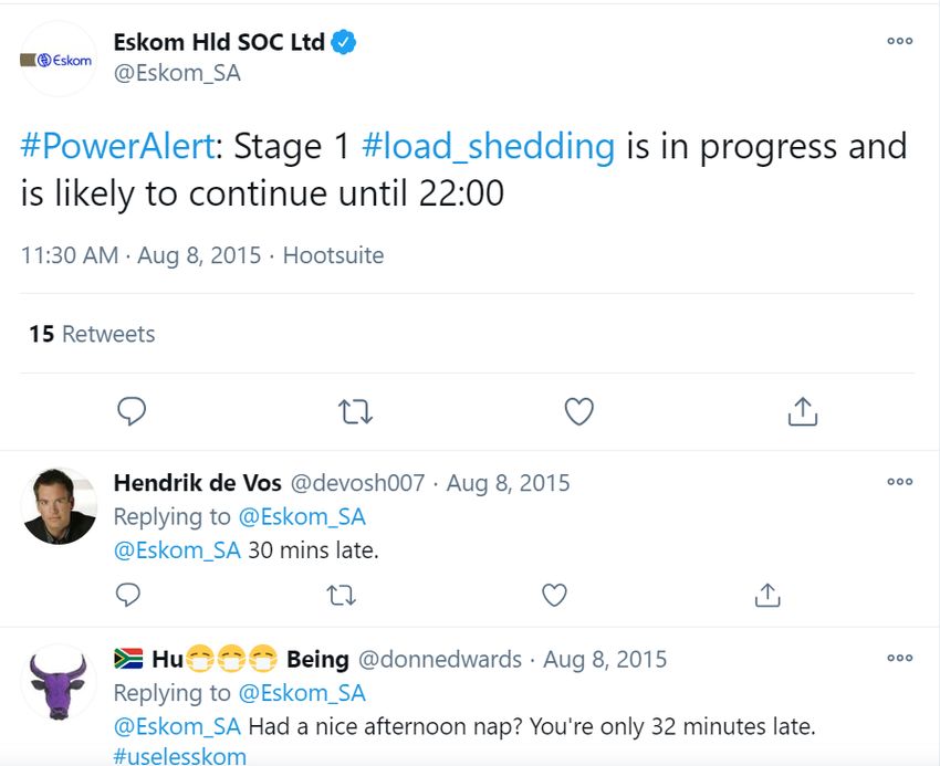
The timing, spacing, and duration of load shedding is seemingly random, at least from the perspective
of a household. Eskom announces load shedding via Twitter and the news, often with very little warning.
In those announcements, the duration of the load shedding, which varies greatly from day to day, is usually
not specified, or incorrect. Finally, to identify which areas experience power outages on load shedding days,
there is a schedule that rotates through the numbered areas by day of the month and hour of the day. For
example, in Figure 1 it shows that on August 8, 2015, Eskom announced over Twitter that load shedding had
already begun by 11:30 AM and would likely continue to 10:00 PM. Individuals would be expected to know
which areas are going to experience power outages in that time frame on the 8th day of the month. Table 1
is an abbreviated version of the load shedding schedule used in Cape Town. On the 8th day of the month,
Areas 11-16 are expected to experience load shedding based on the details in Eskom’s tweet. The final step
is to know which numbered area of Cape Town one is located. For instance, a student of the University of
Cape Town may reside in Area 15 and attend school in Area 7. While campus will not lose power on the
8th, their home will experience a power outage from 6 PM to 8:30 PM. In Figure 1, Eskom mentions that
the load shedding is Stage 1, which means it is the least severe kind of load shedding. As the numbered
stages increase, more areas are added to each 2.5 hour window, like those shown on Table 1, increasing the
probability that areas experience power outages on a given day.
Hand-collected information from Eskom’s tweets in 2014 and 2015 about when load shedding occurred
was combined with Cape Town’s load shedding schedule to determine which areas would experience load
shedding when and for how long. Data on load shedding from just 2014 and 2015 is used even though load
shedding continues to this day. In 2016, there was no load shedding. In 2017, there was a water crisis
and severe drought in Cape Town, and so results including 2017 may capture the effect of the drought on
residential fires, and not load shedding. For 2018 and onwards, there have been multiple issues A variable of
7interest is generated using this method. The variable, LoadSheddingInArea is for if a load shedding area
experienced a power outage on that day based on the times given by Eskom and their eligibility for load
shedding. The second half of Table 2 holds the summary statistics for the residential fire data and load
shedding schedule.
4 Household Energy Consumption
This section reports the changes in household energy consumption in the Western Cape after load shedding.
Though the infrastructural issues occurred at the end of 2014, all respondents in the surveys in the 2015
survey and onward would have experienced load shedding and be aware of the ongoing crisis. Therefore,
respondents of the survey in 2015 and in the following years are considered to be affected by load shedding.
The variable of interest in Tables 3 - 5 is called P ostLoadShedding which a dummy variable that indicates
if the survey response occurred in 2015 or later. The model is as follows:
EnergySourceit = P ostLoadSheddingt + Xit + it
Where the outcome variable, EnergySourceit , is which sources of energy the households indicated they
use for each purpose in a given year. P ostLoadSheddingt is the dummy variable to indicate the year is
greater than or equal to 2015, and Xit is a vector of covariates corresponding with a household in a year such
as, the household’s monthly income, and the age, gender and race of the survey respondent. The General
Household Survey asked respondents to name their main source of energy for cooking, lighting, and heating
in that year. The options are electricity, generators, gas, paraffin, coal, candles, and wood. Some of these
energy sources are only used for a single purpose, like candles are only used for lighting. The outcome
variables are discrete and correlated due to the nature of the survey question’s structure. Therefore, it is
appropriate to use a multinomial logit regression. Multinomial logit regressions are often used in scenarios
when a survey response can be selected from a list of options. Then, one possible answer is used as a reference
point to the other responses. In this case, the coefficient on the variable of interest, P ostLoadSheddingt ,
indicates the change in consumption of an energy source relative to the consumption of electricity after load
shedding begins. For instance, in Table 3 the coefficient in the first column suggests that once load shedding
began, the logit coefficient for generator use, relative to electricity use, will go up by roughly 2.7. In other
words, households are more likely to stay with a generator than switching to electricity. For cooking energy
source, the positive and significant coefficients for generator, gas, paraffin, and wood usage suggests that
8Figure 1: Example of Twitter notification of load shedding
Figure 2: Map of load shedding areas in Cape Town
9Table 1: Abbreviated Load Shedding Schedule Example
Stage 1
Day of Month 1 2 3 4 5 6 7 8 9 10
From To
00:00 02:30 1 13 9 5 2 14 10 6 3 15
02:00 04:30 2 14 10 6 3 15 11 7 4 16
04:00 06:30 3 15 11 7 4 16 12 8 5 1
06:00 08:30 4 16 12 8 5 1 13 9 6 2
08:00 10:30 5 1 13 9 6 2 14 10 7 3
10:00 12:30 6 2 14 10 7 3 15 11 8 4
12:00 14:30 7 3 15 11 8 4 16 12 9 5
14:00 16:30 8 4 16 12 9 5 1 13 10 6
16:00 18:30 9 5 1 13 10 6 2 14 11 7
18:00 20:30 10 6 2 14 11 7 3 15 12 8
20:00 22:30 11 7 3 15 12 8 4 16 13 9
22:00 00:30 12 8 4 16 13 9 5 1 14 10
Table 2: Summary Statistics
Variable Mean St. Deviation Min Max
Cooking = electricity 0.874 0.332 0 1
Cooking = generator 0.021 0.143 0 1
Cooking = gas 0.093 0.291 0 1
Cooking = paraffin 0.013 0.075 0 1
Cooking = wood 0.003 0.054 0 1
Cooking = coal 0.000 0.011 0 1
Lighting = electricity 0.401 0.490 0 1
Lighting = generator 0.003 0.057 0 1
Lighting = gas 0.025 0.155 0 1
Lighting = paraffin 0.013 0.075 0 1
Lighting = candles 0.001 0.035 0 1
Heating = electricity 0.863 0.344 0 1
Heating = generator 0.022 0.149 0 1
Heating = gas 0.006 0.077 0 1
Heating = paraffin 0.013 0.075 0 1
Heating = wood 0.012 0.109 0 1
Heating = wood 0.001 0.109 0 1
Fires per day 0.244 0.560 0 6
Fires in formal dwellings 0.124 0.038 0 4
Fires in informal dwellings 0.120 0.037 0 5
Load shedding day in area 0.002 0.044 0 1
10households were more likely to use those energy sources compared to electricity after load shedding.
Table 4 shows the results regarding the household’s main energy source for lighting. The positive and
significant coefficients for generator, gas, and paraffin mean that households were more likely to continue
using those energy sources, or switch from electricity to those energy sources after load shedding begins.
Table 5 holds the results for the multinomial logit regression where the outcome is a household’s main
energy source for heating. Generator usage for heating is the only positive and significant coefficient for an
alternative energy source. This means that those who were using electricity to heat their homes continued
to do so rather than use another source of energy, like wood, gas, paraffin, or coal. There are a couple
possible explanations for why there are different results for heating energy source compared to cooking and
lighting. First, electric heaters are typically cheaper than gas heaters. On Eskom’s website about heating
options during periods of load shedding, they admit that electric heaters are actually more convenient and
controllable than gas heaters, even if they do not work during periods of load shedding. Additionally, Eskom
recommends to only heat rooms that people are currently spending time in. They discourage the use of wall
mounted heaters, but suggest that fan heaters or air conditioners with a heating cycle could be cost-effective
and energy-conscious ways to heat a home (Eskom, 2020).
The results in Tables 3 - 5 provide evidence that households changed their consumption behavior after
load shedding to alternatives to electricity. The substitutes for electricity are more reliable during the power
outages and are often cheaper than electricity. As household increase their use of wood in place of electricity
for cooking, the risk of house fires also increases. The same could be said for paraffin lamps and stoves, which
pose a higher fire risk than electrical alternatives (Dlamini, 2020). Additionally, electric space heaters also
present an increased fire risk when compared to gas furnaces. Load shedding causes the power to appliances
to switch on and off, which can create power surges. During a power surge, the voltage coming through
to the home can become too high, which degrades the insulation in wires and poses a very serious fire risk
(Qukula, 2015). The results in Tables 3 - 5 suggest that individuals are consuming energy sources that
are more risky in terms of fires because they are cheaper or more reliable during periods of load shedding.
Residential fires are a possible unintended consequence of load shedding because of the patterns in household
energy consumption.
11Table 3: Multinomial Logit Regression Results: Cooking Energy Source
Generator Gas Paraffin Wood Coal
2.677*** 0.189*** 0.094*** 0.911*** -1.193***
Post Load Shedding
(0.000) (0.000) (0.000) (0.000) (0.000)
-0.000*** 0.000*** -0.000*** -0.000*** -0.000
Household monthly income
(0.000) (0.000) (0.000) (0.000) (0.000)
-0.063*** 0.012*** -0.029*** -0.024*** -0.036***
Age of respondent
(0.002) (0.001) (0.004) (0.004) (0.000)
-0.263*** -0.236*** -0.429*** -0.868*** 6.678***
Gender of respondent = female
(0.000) (0.000) (0.000) (0.000) (0.000)
Race of respondent X X X X X
Observations 17,512 17,512 17,512 17,512 17,512
Table 4: Multinomial Logit Regression Results: Lighting Energy Source
Generator Gas Paraffin Candles
2.594*** 0.755*** 1.126*** -9.796***
Post Load Shedding
(0.000) (0.000) (0.000) (0.000)
-0.000*** 0.000*** -0.000*** -0.000
Household monthly income
(0.000) (0.000) (0.000) (0.000)
-0.053*** 0.012*** 0.013*** 0.004
Age of respondent
(0.005) (0.003) (0.001) (0.006)
0.331*** -0.098*** 0.298*** 0.394***
Gender of respondent = female
(0.000) (0.000) (0.000) (0.000)
Race of respondent X X X X
Observations 17,512 17,512 17,512 17,512
Table 5: Multinomial Logit Regression Results: Heating Energy Source
Generator Gas Paraffin Wood Coal
2.397*** -1.751*** -3.434*** -9.889*** -44.643***
Post Load Shedding
(0.000) (0.000) (0.000) (0.000) (0.000)
-0.000*** -0.000 -0.000*** -0.000*** 0.000
Household monthly income
(0.000) (0.000) (0.000) (0.000) (0.000)
-0.060*** -0.005 0.020*** -0.014*** -0.004
Age of respondent
(0.002) (0.003) (0.002) (0.002) (0.035)
-0.240*** -0.355*** 0.260*** -0.316*** 69.587***
Gender of respondent = female
(0.000) (0.000) (0.000) (0.000) (0.001)
Race of respondent X X X X X
Observations 17,512 17,512 17,512 17,512 17,512
125 Residential Fires
A decrease in household consumption of electricity and substitution to other energy sources could have many
unintended consequences. One of the possible consequences is the prevalence of fires. This section of the
article explores the relationship between load shedding and residential fires. The models are as follows:
(1)ResidentialF iresda = P ostLoadSheddingd + Area + M onth + da
(2)ResidentialF iresda = LoadSheddingInAreada + Area + M onth + da
The outcome variable, ResidentialF ires, is the count of fires on a day, by load shedding area. First, the
variable of interest is P ostLoadShedding which indicates that the date in question is after the announcement
of Eskom’s load shedding crisis, December 5, 2014. Then, the variable of interest is LoadSheddingInArea
for if there is load shedding on that day in the load shedding area. Different specifications of the two models
split the data into the count of fires in an area for formal houses only, and then for informal houses only to
see the heterogeneous effects of load shedding on the prevalence of residential fires. The outcome variable is
a discrete count of fires, so it is appropriate to use an ordered logit regression in this case. Tables 6 - 8 show
the results for the ordered logit regression, and determine the likelihood another fire occurring because of
load shedding.
According to Table 6, there were more fires after the information shock about the energy crisis, and
load shedding begins. Additionally, this effect is larger in informal housing than in formal housing. The
variable, In the even numbered columns, the coefficients have been transformed so they can be interpreted
as odds-ratios. For instance, in column 2 of Table 6, after load shedding, an area is 1.159 times more likely
to have one more fire on each day than before load shedding.
In Table 7, the variable of interest is a dummy variable that indicates if an area experienced a power
outage on that day, called LoadSheddingInArea. On days where Eskom implemented load shedding, the
areas that had power outages saw an increase in the prevalence of fires. These effects are stronger for informal
dwellings. Overall, an area was over 50 times more likely to see an additional residential fire on a day when
they experienced load shedding than they otherwise would in the absence of load shedding.
For Table 8, the data is only from the years 2014-2016, excluding 2009-2013. This is because load shedding
was not happening at all from 2009 to 2013, and a goal of this article is to determine if the daily variation
of load shedding had any effect on residential fires. Again, the results suggest that the daily variation of
13load shedding does indeed impact the prevalence of fires. When a load shedding area is experiencing power
outages, there is a greater chance that it will experience one more house fire than it would without load
shedding.
As a check on the previous results, Tables 9 and 10 present the results for a linear probability model
rather than the ordered logit. The results are consistent in sign and significance to the previous tables. This
reinforces the findings that after load shedding began, there were more residential fires. Additionally, there
are more fires in an area on days when Eskom implemented load shedding, and the magnitude of this result
is larger for informal housing. Another advantage to using a linear probability model is ease of interpreting
coefficients. For instance, according to Table 10, on a day when an area had power outages, there were
approximately 1.751 more fires. Of course, there can’t be a fraction of a fire, but when the daily average in
the data is 0.234 for an area, this is a sizable increase. In the data, different areas experience load shedding
110 times, which means there were approximately 193 more fires because of load shedding in a 9 month
period between 2014 and 2015.
Fires are extremely costly to clean up and replace or repair damaged property. In the United States, the
average house fire costs a household over $11,000 (FIXR, 2021). Based prices per sq foot, homes are 1.5 to
4 times more expensive in a US city than in Cape Town (Lippi, 2021)3 . While it is impossible to know the
extent of the damage for these fires, because they were reported to the city and had an emergency response,
it is likely they caused some kind of damage to the residence. 108 of the fires caused by load shedding
occurred in informal dwellings, and the remaining 85 in formal houses. The result is several million Rand
worth of damage caused to individuals due to load shedding.
5.1 Stages of Load Shedding
There are different levels of severity of load shedding, known as stages. As the numbered stages increase,
more load shedding areas are added to each 2.5 hour window on the schedule. For Stage 1, there is one area
per 2.5 hour window, for Stage 2, there are two areas, and so on. Eskom determines what stage to implement
depending on the strain on the grid. In Table 11, there appears to a positive relationship between the stage
of load shedding and the instances of residential fires.
3 The analysis only considers cities of a similar size to Cape Town
14Table 6: Ordered Logit Regression Results: Residential Fires
All Houses Formal Informal
(1) (2) (3) (4) (5) (6)
0.148*** 1.159*** 0.166*** 1.181*** 0.226*** 1.253***
Post Load Shedding
(0.029) (0.029) (0.036) (0.036) (0.037) (0.037)
Area FE X X X X X X
Month FE X X X X X X
Odds-Ratio X X X
Observations 55,587 55,587 55,587 55,587 55,587 55,587
Table 7: Ordered Logit Regression Results: Residential Fires
All Houses Formal Informal
(1) (2) (3) (4) (5) (6)
3.917*** 50.227*** 2.876*** 17.740*** 3.236*** 25.440***
Load Shedding in Area
(0.170) (0.170) (0.178) (0.178) (0.167) (0.167)
Area FE X X X X X X
Month FE X X X X X X
Odds-Ratio X X X
Observations 55,587 55,587 55,587 55,587 55,587 55,587
Table 8: Ordered Logit Regression Results: Residential Fires 2014-16 only
All Houses Formal Informal
(1) (2) (3) (4) (5) (6)
3.712*** 40.926*** 2.755*** 15.725*** 3.095*** 22.086***
Load Shedding in Area
(0.177) (0.177) (0.182) (0.182) (0.174) (0.174)
Area FE X X X X X X
Month FE X X X X X X
Odds-Ratio X X X
Observations 17,241 17,241 17,241 17,241 17,241 17,241
Table 9: Linear Model Results
All Houses Formal Informal
(1) (2) (3)
0.041*** 0.018*** 0.022***
Post Load Shedding
(0.006) (0.004) (0.004)
Area FE X X X
Month FE X X X
Adjusted R-squared 0.092 0.052 0.067
Observations 55,587 55,587 55,587
155.2 Placebo Tests
The results in Table 6 and 9 suggest that there are more fires after load shedding. Perhaps, the results in
Tables 7, 8, and 10 are driven by this change in the prevalence of fires over time, and not daily variation in
load shedding. Placebo tests can help decipher if the previous results are truly being driven by load shedding.
First, in Table 12, the areas are randomly selected to be “treated” with load shedding over the actual 9 month
period where load shedding happened in 2014 and 2015. There is no significant relationship between the
randomly selected areas with load shedding, also known as the placebo treatment, and residential fires.
Next, the exact same days and areas experienced load shedding received the “treatment”, but in the
years 2012 and 2013 instead of 2014 and 2015. There was no load shedding in 2012 and 2013, so if positive
and significant results were to occur from this, then that would mean the previous results are not coming
from the power outages. Table 13 shows that there is no relationship between this placebo treatment of load
shedding and residential fires.
Tables 12 and 13 support the previous results, which find that in areas that experience load shedding on
a given day, there are more residential fires. The findings suggest that the increase in residential fires is due
to the heightened risk of fires caused by the power outages. Individuals in residences during a power outages
are likely to switch to other energy sources to complete daily tasks, which can increase the risk of fires.
There is evidence that people are changing their main source of energy due to load shedding, but individuals
that typically rely on electricity could still switch to a substitute energy source just during periods of load
shedding. Thus, the results in this article about household energy consumption serve as a lower bound
estimate of how individuals respond to load shedding.
Therefore, the increase in the prevalence of residential fires during load shedding is at least in part driven
by changes in changes in energy consumption in response to the power outages. Additionally, load shedding
can cause power surging, which also poses a fire risk (van Niekerk, 2018). The placebo tests provide evidence
that the previous results are being driven by daily and spatial variation in power outages under load shedding.
16Table 10: Linear Model Results
All Houses Formal Informal
(1) (2) (3) (4) (5) (6)
1.751*** 1.691*** 0.776*** 0.751*** 0.975*** 0.940***
Load Shedding in Area
(0.050) (0.053) (0.034) (0.036) (0.035) (0.036)
Area FE X X X X X X
Month FE X X X X X X
2014-2016 only X X X
Adjusted R-squared 0.110 0.168 0.060 0.088 0.079 0.123
Observations 55,587 17,241 55,587 17,241 55,587 17,241
Table 11: Stage of Load Shedding and Residential Fires
All Houses Formal Informal
(1) (2) (3) (4) (5) (6)
-0.013 0.035*** 0.171*** 0.020*** 0.135*** 0.015***
Stage of Load Shedding
(0.037) (0.007 (0.039) (0.005) (0.042) (0.005)
Area FE X X X X X X
Month FE X X X X X X
Ordered Logit Model X X X
Linear Model X X X
Adjusted R-squared – 0.091 – 0.052 – 0.067
Observations 55,587 55,587 55,587 55,587 55,587 55,587
Table 12: Placebo Test: Randomized treatment over load shedding period
All Houses Formal Informal
(1) (2) (3) (4) (5) (6)
Load Shedding Day in Area 0.089 0.028 0.059 0.008 0.358 0.020
(random) (0.245) (0.051) (0.304) (0.034) (0.280) (0.035)
Area FE X X X X X X
Month FE X X X X X X
Ordered Logit Model X X X
Linear Model X X X
Adjusted R-squared – 0.091 – 0.051 – 0.067
Observations 55,587 55,587 55,587 55,587 55,587 55,587
17Table 13: Placebo Test: Same load shedding treatment, but in 2012 & 2013
All Houses Formal Informal
(1) (2) (3) (4) (5) (6)
Load Shedding Day in Area -0.102 -0.057 0.273 0.036 -0.340 -0.093***
(same days, other years) (0.221) (0.051) (0.247) (0.034) (0.350) (0.035)
Area FE X X X X X X
Month FE X X X X X X
Ordered Logit Model X X X
Linear Model X X X
Adjusted R-squared – 0.091 – 0.051 – 0.067
Observations 55,587 55,587 55,587 55,587 55,587 55,587
6 Conclusion
Power outages disrupt daily life, and the literature has shown that they can be quite costly. Scholars are
beginning to understand the unintended consequences of shutting off electricity to reduce strain on the grid,
but none have discussed how there is an increased risk of fire during power outages. Motivated by evidence
of changes in household energy consumption during an energy crisis, this article looks at how power outages
are related to house fires. After the news broke of South Africa’s energy crisis, load shedding became an issue
individuals had to face almost daily. Households were left with the option of using alternative energy sources
or being left in the dark. Using data from Cape Town, South Africa to explore the behavioral responses to
load shedding, there is evidence that significant number of households switched from electricity usage for
cooking and lighting to other sources, like generators, wood and gas. But, there are trade-offs associated
with switching to a more reliable form of energy.
By exploiting plausibly exogenous variation in load shedding timing and spacing, this article captures the
true effect of power outages on residential fires. When an area is experiencing a power outage due to load
shedding, there is an increased likelihood that there will be more residential fires that day. The increased
risk of fires due to the change in household consumption of energy poses an economically significant cost of
load shedding. After load shedding begins, there are significantly more fires in Cape Town. Furthermore,
there were significantly more fires in the areas that were experiencing power outages on a given day. And
finally, while both types of housing classification are adversely affected by load shedding in terms of higher
fire risk, this increased risk is much higher in informal dwellings. This article provides evidence that load
shedding corresponds with an increase in the number of fires in Cape Town, which should be considered as
a cost of the power outages.
18References
Abi Ghanem, D., Mander, S., and Gough, C. (2016). “I think we need to get a better generator”: Household
resilience to disruption to power supply during storm events. Energy Policy, 92:171–180.
Akpandjar, G. and Kitchens, C. (2017). From darkness to light: The effect of electrification in Ghana,
2000–2010. Economic Development and Cultural Change, 66(1):31 – 54.
Anderson, T. B. and Dalgaard, C.-J. (2013). Power outages and economic growth in Africa. Energy Eco-
nomics, 38:19–23.
Anhaeusser, C. J. (2014). Tripped coal stations add to load shedding burden. Fin24.
Beenstock, M. (1991). Generators and the cost of electricity outages. Energy Economics, 13(4):283–289.
Budlender, J. and Royston, L. (2016). Edged out: Spatial mismatch and spatial justice in South Africa’s
main urban areas. Socio-economic rights institute of South Africa.
Byrd, H. and Matthewman, S. (2014). Exergy and the city: The technology and sociology of power (failure).
Journal of Urban Technology, 21(3):85–102.
Carlsson, F., Demeke, E., Martinsson, P., and Tesemma, T. (2020). Cost of power outages for manufacturing
firms in Ethiopia: A stated preference study. Energy Economics, 88.
Carlsson, F. and Martinsson, P. (2008). Does it matter when a power outage occurs? - A choice experiment
study on the willingness to pay to avoid power outages. Energy Economics, 30(3):1232–1245.
Davis, M. (1998). Rural household energy consumption: The effects of access to electricity - evidence from
South Africa. Energy Policy, 26(3):207–217.
de Nooij, M., Lisehout, R., and Koopmans, C. (2009). Optimal blackouts: Empirical results on reducing the
social cost of electricity outages through efficient regional rationing. Energy Economics, 31(3):342–347.
Dlamini, P. (2020). Soweto youth take on Eskom over load shedding: ‘i don’t think they take us seriously’.
City Press.
FIXR (2021). How much does it cost to recover from fire damage? FIXR.
Gehringer, C., Rode, H., and Schomaker, M. (2018). The effect of electrical load shedding on pediatric
hospital admissions in South Africa. Epidemiology, 29(6):841–847.
19Gibbs, J. (2014). Watch Majuba power station seconds before silo collapse (video). The Citizen.
Goldberg, A. (2015). The economic impact of load shedding: The case of South African retailers. University
of Pretoria, Master’s Thesis.
Harish, S. M., Morgan, G. M., and Subrahmanian, E. (2014). When does unreliable grid supply become
unacceptable policy? Costs of power supply and outages in rural India. Energy Policy, 68:158–169.
Hensher, D. A., Shore, N., and Train, K. (2014). Willingness to pay for residential electricity supply quality
and reliability. Applied Energy, 115(15):280–292.
Kazmi, H., Mehmood, F., Zhenmin, T., Riaz, Z., and Driesen, J. (2019). Electricity load-shedding in
Pakistan: Unintended consequences, opportunities and policy recommendations. Energy Policy, 128:411–
417.
Klinger, C., Landeg, O., and Murry, V. (2014). Power outages, extreme events and health: A systematic
review of the literature from 2011-2012. PLOS Currents Disasters, 1.
Lawson, K. (2021). Effect of electrical outages on educational outcomes: Load shedding in South Africa.
Working Paper.
Lippi, K. (2021). Apartment prices across the world. I Sold My House.
Ndaguba, E. (2017). Load shedding and community health centres in South Africa: A conceptual scholarship
(2014 – 2016). Etho Medicine.
Neilson, A. (2017). The socio-political importance of blackouts in South Africa. Social Space.
Niselow, T. (2019). Sunday read: Load shedding through the years and how Eskom has struggled to keep
the lights on. Fin24.
Pieterse, E. (2009). Post-Apartheid geographies in South Africa: Why are urban divides so persistent?
Interdisplinary Debates on Development and Cultures: Cities in development-spaces.
Pretorius, I., Piketh, S., and Burger, R. (2015). The impact of the South African energy crisis on emissions.
Air Pollution.
Qukula, Q. (2015). Fire risks after load shedding and who foots the bill. 702.
20Rose, A., Oladosu, G., and Liao, S. (2007). Business interruption impacts of a terrorist attack on the electric
power system of Los Angeles: Customer resilience to a total blackout. Risk Analysis, 27(3):513–531.
Sue Wing, I. and Rose, A. Z. (2020). Economic consequence analysis of electric power infrastructure disrup-
tions: General equilibrium approaches. Energy Economics, 89.
van Niekerk, M. (2018). Load shedding poses a significant fire-safety risk, warns fire expert. ASPFire.
Wijayatunga, P. and Jayalath, M. (2004). Assessment of economic impact of electricity supply interruptions
in the Sri Lanka industrial sector. Energy Conversion and Management, 45:235–247.
Wilkinson, P. (1998). Housing policy in South Africa. Habitat International, 22(3).
Zachariadis, T. and Poullikkas, A. (2012). The costs of power outages: A case study from Cyprus. Energy
Policy, 51:630–641.
21You can also read