Analysis of Travel Hot Spots of Taxi Passengers Based on Community Detection
←
→
Page content transcription
If your browser does not render page correctly, please read the page content below
Hindawi
Journal of Advanced Transportation
Volume 2021, Article ID 6646768, 14 pages
https://doi.org/10.1155/2021/6646768

Research Article
Analysis of Travel Hot Spots of Taxi Passengers Based on
Community Detection

 Shuoben Bi ,1 Yuyu Sheng,1 Wenwu He,2 Jingjin Fan,3 and Ruizhuang Xu1
 1
 School of Geographical Sciences, Nanjing University of Information Science & Technology, No. 219 Ningliu Road,
 Nanjing 210044, China
 2
 Mathematics and Physics Institute, Fujian University of Technology, No. 33 Xuefu South Road, University New District,
 Fuzhou 350001, China
 3
 Institute for the History of Science and Technology, Nanjing University of Information Science & Technology,
 No. 219 Ningliu Road, Nanjing 210044, China

 Correspondence should be addressed to Shuoben Bi; bishuoben@163.com

 Received 12 November 2020; Revised 6 March 2021; Accepted 16 March 2021; Published 26 March 2021

 Academic Editor: Xinyue Xu

 Copyright © 2021 Shuoben Bi et al. This is an open access article distributed under the Creative Commons Attribution License,
 which permits unrestricted use, distribution, and reproduction in any medium, provided the original work is properly cited.
 It is an important content of smart city research to study the activity track of urban residents, dig out the hot spot areas and spatial
 interaction patterns of different residents’ activities, and clearly understand the travel rules of urban residents’ activities. This study
 used community detection to analyze taxi passengers’ travel hot spots based on taxi pick-up and drop-off data, combined with
 multisource information such as land use, in the main urban area of Nanjing. The study revealed that, for the purpose of travel, the
 modularity and anisotropy rate of the community where the passengers were picked up and dropped off were positively correlated
 during the morning and evening peak hours and negatively correlated at other times. Depending on the community structure,
 pick-up and drop-off points reached significant aggregation within the community, and interactions among the communities
 were also revealed. Based on the type of land use, as passengers’ travel activity increased, travel hot spots formed clusters in urban
 spaces. After comparative verification, the results of this study were found to be accurate and reliable and can provide a reference
 for urban planning and traffic management.

1. Introduction Time-space analysis based on residents’ activities can
 explain the homogeneity of the influence of individual resi-
With the rapid development of information technology, dents’ behaviors on urban space, and the behaviors between
spatial analysis driven by data forces geographic information different individuals can reflect that they are restricted by
science to face new challenges. Furthermore, visual analysis urban space and show their differences [3]. Therefore, as
combined with geographic computing has greatly improved Harvey and Han [4] proposed the concept of geographic data
people’s ability to mine new knowledge [1]. On the one mining and knowledge discovery, scholars have continued to
hand, mobile information collection technology based on explore knowledge in recent decades, and geography has
the global positioning system has become more mature; on experienced transition from an empirical paradigm to a
the other hand, the flow space with urban residents’ activities system simulation paradigm and then to a data-driven par-
as the main carrier has become more extensive [2]. Although adigm [5]. Early research on the behavioral patterns of urban
the intension of geographic information science has not residents’ activities mainly focused on extracting residents’
changed, its content and form have become richer. There- activity points and on the correlation analysis of those points.
fore, breaking through the traditional urban spatial research For example, Veloso et al. [6] studied the strong association
model is the key to discovering the law of urban residents’ pattern of residents’ activity locations, and Ahas et al. [7]
activities. studied the time difference and spatial distribution of
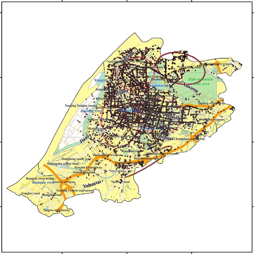
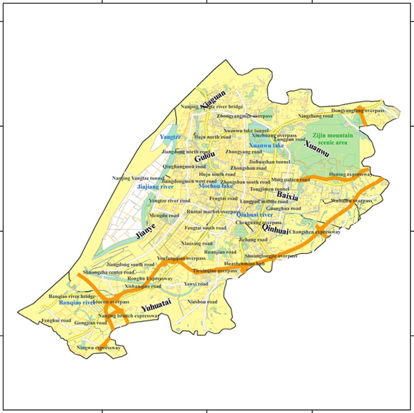
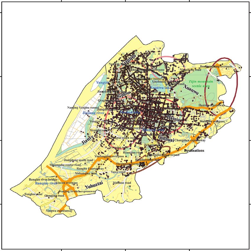
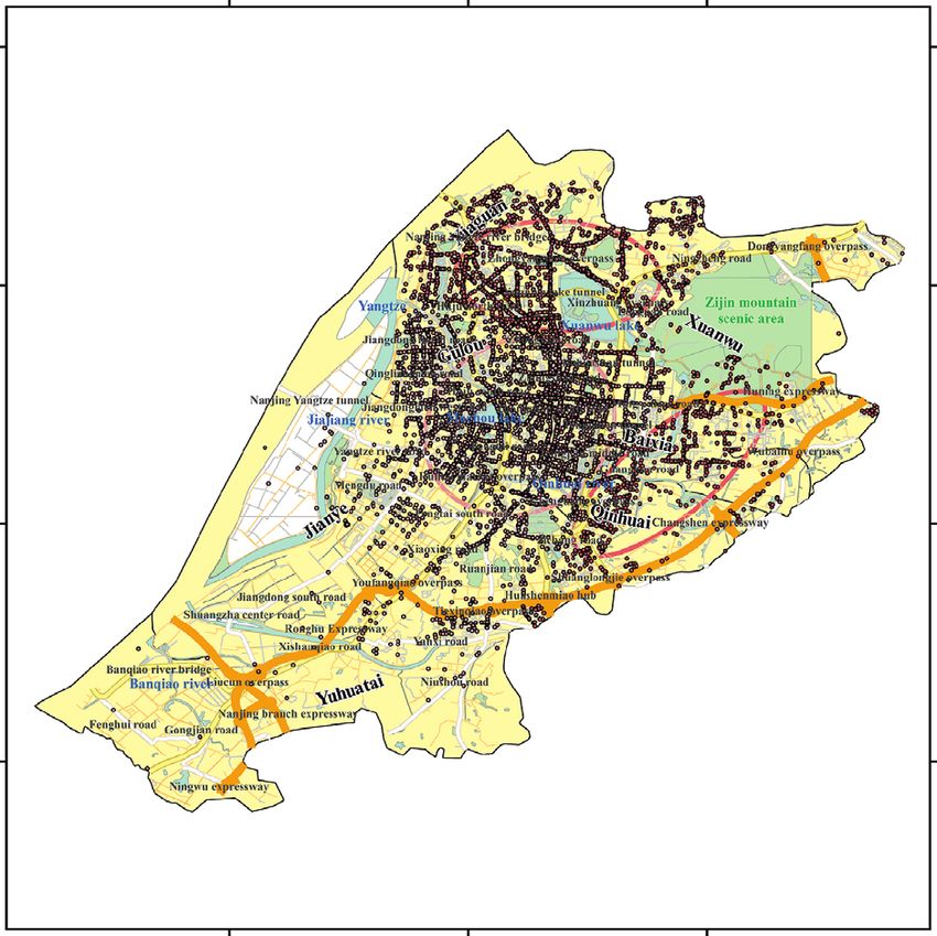
2 Journal of Advanced Transportation

residents’ activities. Recent research has mainly focused on 2. Data Description
the identification of urban hot spot functional areas, urban
accessibility analysis, urban boundary division, polycentric Nanjing is located in the southwest of Jiangsu Province,
evaluation, etc. For example, Scholz et al. [8] studied urban China. The study area selected in this paper covers the main
residents’ behavioral patterns and the temporal and spatial urban area of Nanjing, including Gulou, Xuanwu, Jianye,
development of urban hot spots, and Cui et al. [9] studied the Qinhuai, and Yuhuatai, as shown in Figure 1.
accessibility of urban residential areas and the distribution of The data used in this study includes two parts of the
low-access residential areas. Zhong et al. [10] studied the Nanjing taxi trajectory and feature dataset. The source of
overall spatial structure of changes in the center of the city Nanjing taxi trajectory data was Datatang (https://www.
boundary, and Huang et al. [11] studied the effects of urban datatang.com), which contains data from approximately
traffic and pedestrian activities. For two-layer fine-grained 7,800 taxis with a sampling interval of 30 seconds. Data for
networks, Guo et al. [12] studied the structure of different the same period for three consecutive years were selected:
urban road networks and developed corresponding datasets. January 25–31, 2015; February 13–19, 2016; and February
Hamedmoghadam et al. [13] studied the displacement index 2–8, 2017. The source of road network data was Tianditu
of individual travel granularity to simplify collective behav- (https://www.tianditu.gov.cn), a national geographic infor-
ioral patterns. In addition, there are related studies on urban mation public service platform, which contains eight types of
planning and environmental safety assessment. For example, graded roads. Considering the nature of taxi services, rail-
Zheng et al. [14] studied the characteristics of cross con- ways, subways, light rails, and high-speed rails were ex-
nectivity between urban planning and taxi driving, and Wu cluded. Approximately 2,400 road sections classified as
et al. [15] studied the temporal and spatial patterns of urban national roads, provincial roads, county roads, township and
road traffic accidents. village roads, and other roads were used in the analysis. The
 In summary, the early research model was relatively data source of points of interest was Baidu POI (http://www.
narrow in its scope, only considering residents’ activities but data-shop.net/tag/), which includes four types of land use:
ignoring the characteristics of urban space. In recent years, land for commercial use, residential land, land for public
research has become relatively rich, mainly based on urban management and public service, and land for transportation.
planning, which was based on the analysis of residents’ A total of approximately 26,000 points of interest were
historical activities, such as behavioral patterns. The land- selected.
mark research achievements are the GN algorithm [16] and
the Newman fast algorithm [17], both of which are classic 3. Methodology
community detection algorithms. These can fully reveal the
different resident activities, the spatial pattern, and the This study used ArcGIS to perform map matching and
impact of potential factors on decision-making. In addition, geocoding preprocessing on taxi movement trajectories and
Qin et al. [18] studied the traffic intensity and edge weight of the feature data of Nanjing City. A road network geographic
network nodes based on the network interaction charac- database and a road network topology map were created
teristics of urban hot spots. using the complex network-modeling tool NetworkX to map
 The movement trajectory as a type of multisource sensor the road intersections. The abstraction of the road inter-
data has been widely adopted by researchers. Through the sections is a complex network node, the corresponding road
movement trajectory, the travel mode of residents’ activities section is abstracted as an edge, and community detection is
can be understood more clearly, the hot spots of activities performed on the taxi pick-up and drop-off points. Based on
can be extracted more accurately, and the reasons for the community detection, the passenger travel activity index is
resident movement can be analyzed. Research on moving constructed, and hot spot mining is realized through spatial
trajectories in Nanjing mainly includes Xu et al. [19], who statistics. The technical process is shown in Figure 2.
found that traffic hot spots in Nanjing have the spatial
distribution characteristics of agglomeration from the sur- 3.1. Community Detecting. First, based on the concept of a
roundings to the center; Yang et al. [20], who found that the dual graph [22], the road is defined as a generalized network
Nanjing public transport system has the characteristics of composed of nodes and edges.
cascading failure congestion; and Jin and Xu [21], who
showed that the traffic flow on the key nodes of different G � Ng , Eg |1 ≤ g ≤ nGraph ,

grades of road network in Nanjing has obvious hierarchical N � n , (1)
 g node
structure characteristics. Therefore, this study aims to use
the passenger pick-up and drop-off points extracted from E � n ,
 g edge
taxi movement trajectories to explore the travel rules of taxi
passengers, analyze the time and space patterns of taxi pick- where (Ng , Eg ) represents any road segment, nGraph rep-
up and drop-off communities, establish passenger travel resents the total number of road segments, nnode represents
activity indicators based on community detection [16], the number of nodes included in a road segment, and nedge
combine the data of graded roads and points of interest, represents the number of edges included in a road segment.
explore the temporal and spatial characteristics of taxi The road is abstracted into a complex network, as shown
passenger travel hot spots, and examine the causes of the in Figure 3: (a) is the original road graph, which contains 9
formation of spatiotemporal characteristics. road sections and 14 nodes; (b) is the corresponding original
Journal of Advanced Transportation 3

 118°30′0″E 119°0′0″E 118°40′0″E 118°45′0″E 118°50′0″E

 32°10′0″N

 32°10′0″N
 N Nanjing N Study area
 32°30′0″N

 32°30′0″N
 32°5′0″N

 32°5′0″N
 32°0′0″N

 32°0′0″N

 32°0′0″N
 32°0′0″N
 31°30′0″N

 31°30′0″N
 31°55′0″N

 31°55′0″N
 (km) (km)
 0 5 10 0 5 10

 118°30′0″E 119°0′0″E 118°40′0″E 118°45′0″E 118°50′0″E

 Lable Xuanwu State road Green space
 Nanjing Jianye Procincial road River system
 Study area Baixia Country road Island
 Xiaguan Qinhuai Village road Administrative division
 Gulou Yuhuatai Other road
 Figure 1: Study area map.

 Taxi GPS data Land use data

 Data preprocessing

 Map matching and geocoding

 Building complex networks based on dual graph

 Evaluating the community of pick-up and drop-
 Community detecting
 off points based on modularity

 Modeling relationships between communities

 Constructing index of passenger travel activity
 Passenger travel hot
 spot analysis
 Measuring passenger activity space based on
 anisotropy rate

 Figure 2: Technical flowchart.
4 Journal of Advanced Transportation

 1 1 1
 5 7 9 7
 2 2 2 2 5 9
 2
 6 8

 5 3 9 3
 6 8

 6 8

 4 4 4
 4
 (a) (b) (c)

Figure 3: Diagram of a complex network of roads: (a) road network graph; (b) road network initialization graph; (c) road network dual
graph.

graph, where the nodes represent road intersections and the where Ci and Cj are the clusters where the pick-up points SO i
edges represent road sections between nodes; (c) is the and SOj are located; ni and nj are the number of pick-up
corresponding dual graph, in which nodes represent road points contained in clusters Ci and Cj , respectively; and
sections and edges represent the intersecting relationship of |Qi − Qj | is the distance between clusters Ci and Cj . Q is the
road sections. incremental matrix, which is the adjacency matrix that stores
 Figure 3(c) is used to abstract the road network and the nodes and edges within the cluster. Q is calculated as
express intersections and road sections as nodes and edges, follows [24]:
respectively. Before community detection, the stay points are
 1 ki kj
mapped to the road network, which characterizes the geo- Q� − , (4)
graphic location using map matching technology. After Eg 2E2g
abstraction, the road network not only retains the geo-
graphic location information but also characterizes the where Eg is the total number of connected edges, ki is the
network connectivity. The connectivity of the road network degree of node i, and kj is the degree of node j.
changes with the degree centrality of each node in the ab- For a network with N nodes, the execution process of the
stract network. The more the pick-up points, the higher the algorithm used in this study includes the following steps:
exit degree of the node, and the more the drop-off points, the (1) Initializing. Treat each node as a cluster and set the
higher the entry degree of the node. Therefore, when the stay increment matrix to Q � 0.
points change dynamically in the road network, they are
 (2) Merging and Updating. Combine the two clusters Ci
aggregated into clusters according to Bayes’ rule, and
 and Cj that have edges connected in such a way that
communities are established to represent the activities of the
 maximizes davg , maximize davg using Bayes’ rule, and
community’s residents as hot spots.
 update the combined cluster.
 Second, we define the stay point, corresponding to the
stay point to the network, and use it as a separate atomic (3) Terminating. Continue the merging and updating
cluster [23]. process until there are no clusters that can be
 merged.
 S � SO D
 i , Si | 1 ≤ i ≤ NS , (2) We then count the number of pick-up points in each
 cluster as the amount of information I and set the amount of
where (SO D
 i , Si ) represents any pair of stay points, NS rep- information as the weight according to Bayes’ rule, thereby
resents the number of stay points included in the candidate establishing a community as
dataset, SO represents the pick-up point in a pair of stay
points, and SD represents the drop-off point in a pair of stay 1 n i
 I� C ,
points. n i�1 ni
 Subsequently, the distance between the stay points is
calculated according to the Euclidean metric. Taking the n P I/ni × P ni
above stay points as an example (the same is true for the P i � , (5)
 I P ni × P I/ni + P ni × P I/ni
drop-off point), the two closest points are continuously
merged into the same cluster, and the distance between the ni�1 xi , yi × P ni /I
clusters is calculated according to the average distance Bi � ,
 ni�1 P ni /I
measurement:
 1 where Cini means that the cluster Ci in the community
 davg Ci , Cj � Qi − Qj , (3) contains ni pick-up points, and n is the total number of pick-
 nn
 i j Qi ∈Ci Qj ∈Cj
 up points in the community. P(ni /I) means that the pick-up
Journal of Advanced Transportation 5

points are aggregated into the pick-up point community, where di is the distance between taxi passengers’ pick-up and
and (xi , yi ) denotes the coordinates of the pick-up points. Bi drop-off points, Ri is the smallest radius of the circle that
is the center of the mass coordinates of community (xB , yB ). contains the community of the pick-up point, nO denotes all
 Finally, the community is evaluated according to the pick-up points included in the pick-up point community,
degree of modularity M: and nD denotes all drop-off points included in the drop-off
 ki kj point community. scopei is a probability density function
 1
 M� Cij − z Bi , Bj , (6) that describes the distance between the pick-up point and
 2E ij 2E the centroid of the community it belongs to; departi rep-
 resents the probability density estimation from the pick-up
where E is the number of edges in the network. Cij takes the point to the pick-up point community, namely, the popu-
value 0 or 1; if Cij � 1, there is an edge between the pick-up larity of passenger outbound travel activities; arrivei rep-
points SO O
 i and Sj ; otherwise, there is no edge; ki and kj are resents the probability density estimation from the drop-off
the degrees of the pick-up points SO O
 i and Sj ; Bi and Bj are the point to the drop-off point community, that is, the popu-
centroids of the communities where the pick-up points SO i larity of passenger arrival travel activities.
and SOj are located. Only when Bi � Bj , z(Bi , Bj ) � 1. The Given N nodes, there can be at most N(N − 1)/2 edges,
value range of M is [0, 1]; the larger the value, the more and a random network can be obtained by randomly
obvious the community structure. selecting M edges from these edges. Obviously, a total of
 CMN(N−1)/2 random graphs are possible, each with the same
 probability. When the node’s connection probability p ex-
3.2. Constructing an Indicator of Passenger Travel Activity. ceeds the critical probability pc (N) � ln N/N, every random
Based on the community detection results, the passenger graph is connected. Therefore, a random graph Q with N
travel activity point is set as Si � [SO D O D O
 i , Si , Bi , Bi ], where Si is nodes and connection probability p � p(N) satisfies
 D
the coordinate of the taxi passenger pick-up point, Si is the
coordinate of the drop-off point, BO 1, p(N)/pc (N) ⟶ ∞,
 i is the centroid coor- lim PN,p (Q) � (8)
dinate of the community to which the pick-up point belongs, N⟶∞ 0, p(N)/pc (N) ⟶ 0.
and BD i is the centroid coordinate of the community to
which the drop-off point belongs. Therefore, there are three For the community of pick-up and drop-off points
situations of inclusion, intersection, and separation of the formed by the corresponding pick-up and drop-off points,
communities, in which the passenger board and drop-off when p(N)/pc (N) ⟶ ∞, the random network is com-
points belong, as shown in Figure 4. pletely connected, forming a closed network with no isolated
 As shown in Figure 4, the center of the pick-up point nodes. In other words, the pick-up point will not belong to
community is O and the radius is rO ; the center of the drop- the community of the drop-off points, and the drop-off point
off point community is D and the radius is rD ; and the will not belong to the community of the pick-up points,
smallest circle center that contains the pick-up point namely, SO
 i ∉ ⊙ Bi
 D
 and SD O
 i ∉ ⊙ Bi . When
community is C and the radius is R. No interaction between p(N)/pc (N) ⟶ 0, the random network has a tree struc-
the pick-up point community and the drop-off point ture, and there are branch nodes belonging to other con-
community is shown by the white area in the figure, while an nected subgraphs, namely, SO D D O
 i ∈ ⊙ Bi or Si ∈ ⊙ Bi .
interaction between the pick-up point community and the Because passengers are not necessarily restricted to
drop-off point community is shown by the shaded area in moving in certain pairs of communities, the standard de-
the figure. viation ellipse method [26] is used to measure the spatial
 The passenger travel activity index is a combination of distribution characteristics of passenger activities and the
outbound visit heat and arrival visit heat [25], with 1 h as the interaction of the community where the passengers travel
unit time for sampling and 1 km as the unit distance for activity points are evaluated according to the anisotropy rate,
calculation, defined as Ai � [departi , arrivei ]; the calcula- that is, an equal ellipse. The higher the anisotropy rate under
tion is as follows: the area, the more directional and purposeful the passenger
 activities in the community. The anisotropy rate α is cal-
 di
 scopei � 1 − , culated as follows:
 2Ri
 σ x′ − σ y′
 O D D O α� × 100%, (9)
 ⎧
 ⎪
 ⎨ 1, Si ∉ ⊙ Bi 且Si ∉ ⊙ Bi , σ x′
 p Si ∈ Bi � ⎪
 ⎩ 0, O ∈ ⊙ BD 或SD ∈ ⊙ BO , where σ x′ is the length of the major axis of the ellipse and σ y′
 i i i i
 (7) is the length of the minor axis of the ellipse.
 nO
 departi � p SO O O
 i ∈ ⊙ Bi × scopei ,
 SO O
 i ∈ Bi
 4. Results and Analysis
 nD 4.1. Spatial and Temporal Characteristics of Passenger Travel
 arrivei � p SD D D
 i ∈ ⊙ Bi × scopei , Activity. One hour was adopted as the unit time interval to
 SD D
 i ∈ Bi summarize the passenger pick-up and drop-off points
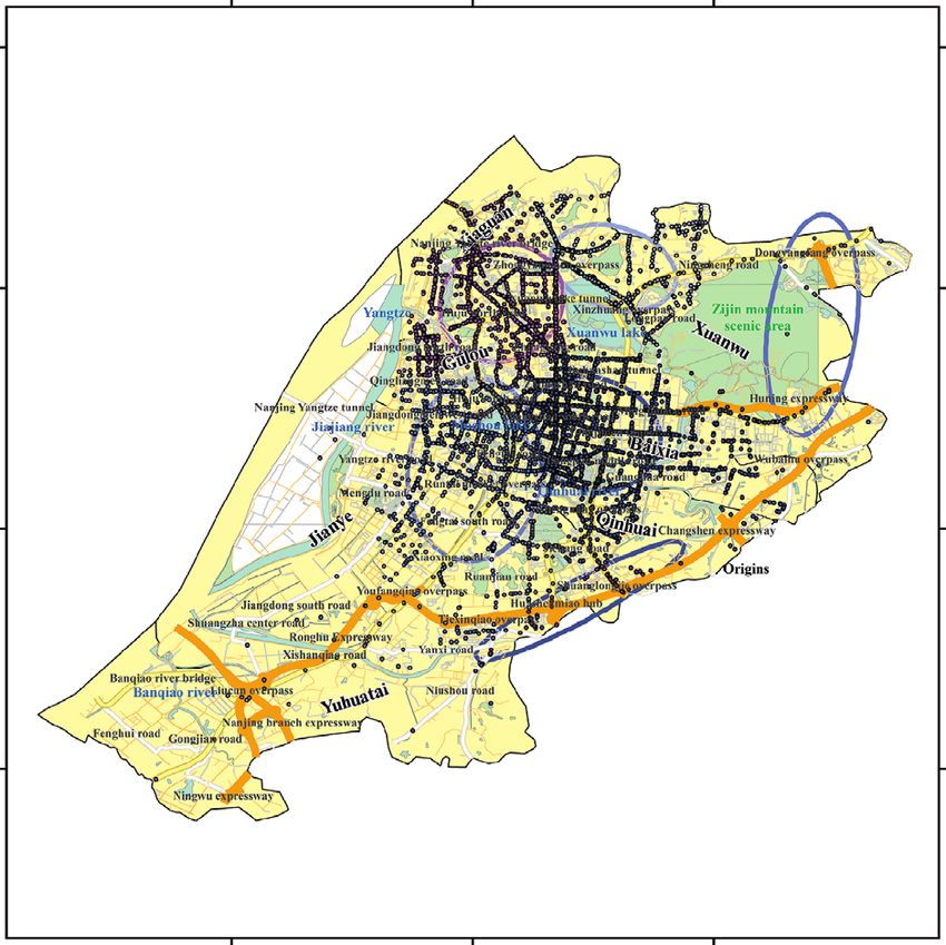
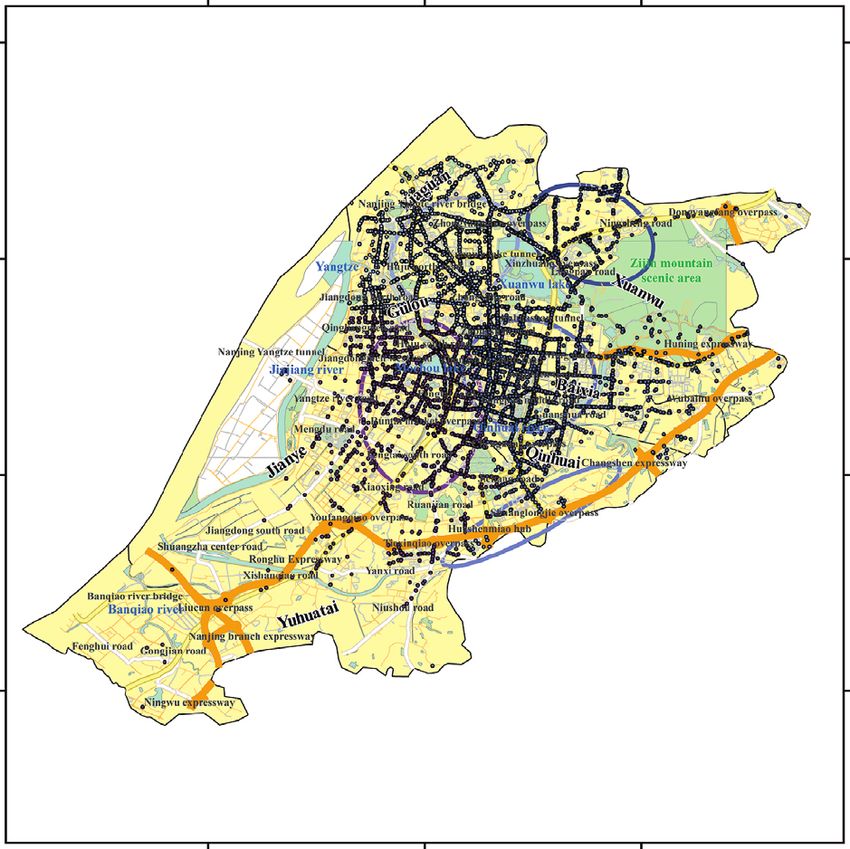
6 Journal of Advanced Transportation

 O O
 O O O
 D C C
 D C C C
 D
 D
 D

 0 ≤ |OD| < |rO – rD| |OD| = |rO – rD| |rO – rD| < |OD| < |rO + rD| |OD| = |rO + rD| |OD| > |rO + rD|
 Inside Inscribed Intersecting Circumscribed Outside

 Community inclusion Community intersecting Community separation
 C = IF(rO > rD, O, D) C = AVERAGE(O, D) C = AVERAGE(O, D)
 R = MAX (rO, rD) R = IF(rO > rD, CO + rO, CD + rD) R = IF(rO > rD, CO + rO, CD + rD)

Figure 4: Schematic diagram of three community situations. Note. The blue circle represents the taxi pick-up community, its center is O,
and its radius is rO. The green circle represents the taxi drop-off community, its center is D, and its radius is rD. The red circle represents the
smallest circumscribed circle that contains two communities, its center is C, and its radius is R. In the case of community inclusion, if rO > rD,
then C is O; otherwise, C is D. The value of R is maximum in rO and rD. In the case of community intersection or community separation, the
value of C is average of O and D coordinates. If rO > rD, then the value of R is the sum of the values of CO (distance value between C and O)
and rO; otherwise, the value of R is the sum of the values of CD (distance value between C and D) and rO.

recorded in the taxi trajectory data for the weeks included in
 Passenger volume/number
 16000
the data analysis (Section 2), as shown in Figure 5. 14000
 It can be seen from Figure 5 that the number of taxi 12000
 10000
passengers getting on and off is consistent across days of the 8000
week, and there are fluctuations at different times of the day. 6000
The daytime is higher than the nighttime, and there is a 4000
significant increase during the morning rush hour. More- 2000
 0
over, there is also a certain increase during the evening rush
 00:00-01:00
 01:00-02:00
 02:00-03:00
 03:00-04:00
 04:00-05:00
 05:00-06:00
 06:00-07:00
 07:00-08:00
 08:00-09:00
 09:00-10:00
 10:00-11:00
 11:00-12:00
 12:00-13:00
 13:00-14:00
 14:00-15:00
 15:00-16:00
 16:00-17:00
 17:00-18:00
 18:00-19:00
 19:00-20:00
 20:00-21:00
 21:00-22:00
 22:00-23:00
 23:00-24:00
hour. Thus, taxi passenger travel show more daytime ac-
tivity, less nighttime activity, and frequent activity during
the morning and evening peak hours.
 Taking one hour as the unit time interval, the average Time
modularity and anisotropy rate of the communities where Sunday Thursday
taxi passengers were picked up and dropped off in 2015, Monday Friday
2016, and 2017 are shown in Figure 6. Tuesday Saturday
 It can be seen from Figure 6 that, during the morning Wednesday
and evening peak hours, the modularity is relatively high, Figure 5: Graph of average passenger volume.
and the anisotropy rate curve is relatively steep. When the
modularity increases, the anisotropy rate also increases. In
other periods, the modularity is relatively low, and the up and drop-off points are mainly intersecting. The pick-
anisotropy rate curve is relatively flat. When the modularity and-drop points, as shown in Community No. 1
decreases, the anisotropy rate increases. This shows that the (Figure 7(b)), are mainly gathered in the southeast of Gulou,
community structure of taxi passengers’ pick-up and drop- southwest of Xuanwu, west of Qinhuai, and northeast of
off points becomes closer as the purpose of passengers’ travel Jianye area. During the period of 18 : 00–19 : 00, the corre-
increases. For example, during morning peak hours, pas- sponding communities of the pick-up and drop-off points
sengers travel mainly from home to office; during evening are mainly separate. During 22 : 00–23 : 00 (Figure 7(d)), the
peak hours, passengers travel mainly from office to home; corresponding communities of the pick-up and drop-off
and in other periods, residents’ activities are affected by points are mainly inclusive. The pick-up and drop-off points
differences in travel motivation, thus showing randomness. shown in Community No. 1 are mainly concentrated in the
 To clearly reflect the differences in residents’ travel ac- northwest of Xuanwu, and the pick-up and drop-off points
tivities at different times, the morning peak hours were 8 : shown in Community No. 2 are mainly concentrated in
 00–9:00, working hours 13 : 00–14 : 00, evening peak hours Jianye. In the northeast, the pick-up and drop-off points
18 : 00–19 : 00, and rest period 22 : 00–23 : 00. We can con- shown in Community No. 5 are mainly concentrated in the
duct community detection at the points where taxi pas- northeast of Yuhuatai, and the pick-up and drop-off points
sengers board and alight, as shown in Figure 7. shown in Community No. 6 are mainly concentrated in the
 It can be observed from Figure 7 that during the period middle of Gulou.
of 8 : 00–9:00, the corresponding communities of the pick- This shows that, during the same period, passenger travel
up and drop-off points are separate, and during the period of activities are affected by the purpose of travel, showing the
13 : 00–14 : 00, the corresponding communities of the pick- same behavioral pattern in the same community, obvious
Journal of Advanced Transportation 7

 0.900 22.00
 21.00
 0.850 20.00

 Anisotropy rate (%)
 19.00
 0.800

 Modularity
 18.00
 0.750 17.00
 16.00
 0.700 15.00
 14.00
 0.650
 13.00
 0.600 12.00
 00:00-01:00
 01:00-02:00
 02:00-03:00
 03:00-04:00
 04:00-05:00
 05:00-06:00
 06:00-07:00
 07:00-08:00
 08:00-09:00
 09:00-10:00
 10:00-11:00
 11:00-12:00
 12:00-13:00
 13:00-14:00
 14:00-15:00
 15:00-16:00
 16:00-17:00
 17:00-18:00
 18:00-19:00
 19:00-20:00
 20:00-21:00
 21:00-22:00
 22:00-23:00
 23:00-24:00
 Time

 Modularity
 2015 year 2016 year 2017 year
 Anisotropy rate
 Figure 6: Graph of average community modularity and anisotropy rate.

 118°40′0″E 118°45′0″E 118°50′0″E 118°40′0″E 118°45′0″E 118°50′0″E
 32°10′0″N

 32°10′0″N

 32°10′0″N

 32°10′0″N
 N N
 Community detection of origins Community detection of destinations
 from 8:00 to 9:00 from 8:00 to 9:00
 32°5′0″N

 32°5′0″N

 32°5′0″N

 32°5′0″N
 32°0′0″N

 32°0′0″N

 32°0′0″N

 32°0′0″N
 31°55′0″N

 31°55′0″N

 31°55′0″N

 31°55′0″N
 0 5 10 (km) 0 5 10 (km)

 118°40′0″E 118°45′0″E 118°50′0″E 118°40′0″E 118°45′0″E 118°50′0″E
 Origins Taxi pick-up community Destinations Taxi drop-off communities
 Origins in no.1 community No.1 community Destinations in no.1 community No.1 community
 Origins in no.2 community No.2 community Destinations in no.2 community No.2 community
 Origins in no.3 community No.3 community Destinations in no.3 community No.3 community
 Origins in no.4 community No.4 community Destinations in no.4 community No.4 community
 (a)
 Figure 7: Continued.
8 Journal of Advanced Transportation

 32°10′0″N 118°40′0″E 118°45′0″E 118°50′0″E 118°40′0″E 118°45′0″E 118°50′0″E

 32°10′0″N

 32°10′0″N

 32°10′0″N
 N N
 Community detection of origins Community detection of destinations
 from 13:00 to 14:00 from 13:00 to 14:00
 32°5′0″N

 32°5′0″N

 32°5′0″N

 32°5′0″N
 32°0′0″N

 32°0′0″N

 32°0′0″N
 32°0'0″N
 31°55′0″N

 31°55′0″N

 31°55′0″N
 31°55'0″N
 0 5 10(km) 0 5 10(km)

 118°40′0″E 118°45′0″E 118°50′0″E 118°40′0″E 118°45′0″E 118°50′0″E

 Origins Taxi pick-up communities Destinations Taxi drop-off communities
 Origins in no.1 community No.1 community Destinations in no.1 community No.1 community
 Origins in no.2 community No.2 community Destinations in no.2 community No.2 community
 Origins in no.3 community No.3 community Destinations in no.3 community No.3 community
 (b)
 118°40′0″E 118°45′0″E 118°50′0″E 118°40′0″E 118°45′0″E 118°50′0″E
 32°10′0″N

 32°10′0″N

 32°10′0″N

 32°10′0″N
 N N
 Community detection of origins Community detection of destinations
 from 18:00 to 19:00 from 18:00 to 19:00
 32°5′0″N

 32°5′0″N

 32°5′0″N
 32°5′0″N

 32°0′0″N

 32°0′0″N

 32°0′0″N
 32°0′0″N
 31°55′0″N

 31°55′0″N

 31°55′0″N

 31°55′0″N

 0 5 10 (km) 0 5 10 (km)

 118°40′0″E 118°45′0″E 118°50′0″E 118°40′0″E 118°45′0″E 118°50′0″E

 Origins Taxi pick-up communities Destinations Taxi drop-off communities
 Origins in no.1 community No.1 community Destinations in no.1 community No.1 community
 Origins in no.2 community No.2 community Destinations in no.2 community No.2 community
 Origins in no.3 community No.3 community Destinations in no.3 community No.3 community
 Origins in no.4 community No.4 community Destinations in no.4 community No.4 community
 Origins in no.5 community No.5 community Destinations in no.5 community No.5 community
 (c)
 Figure 7: Continued.
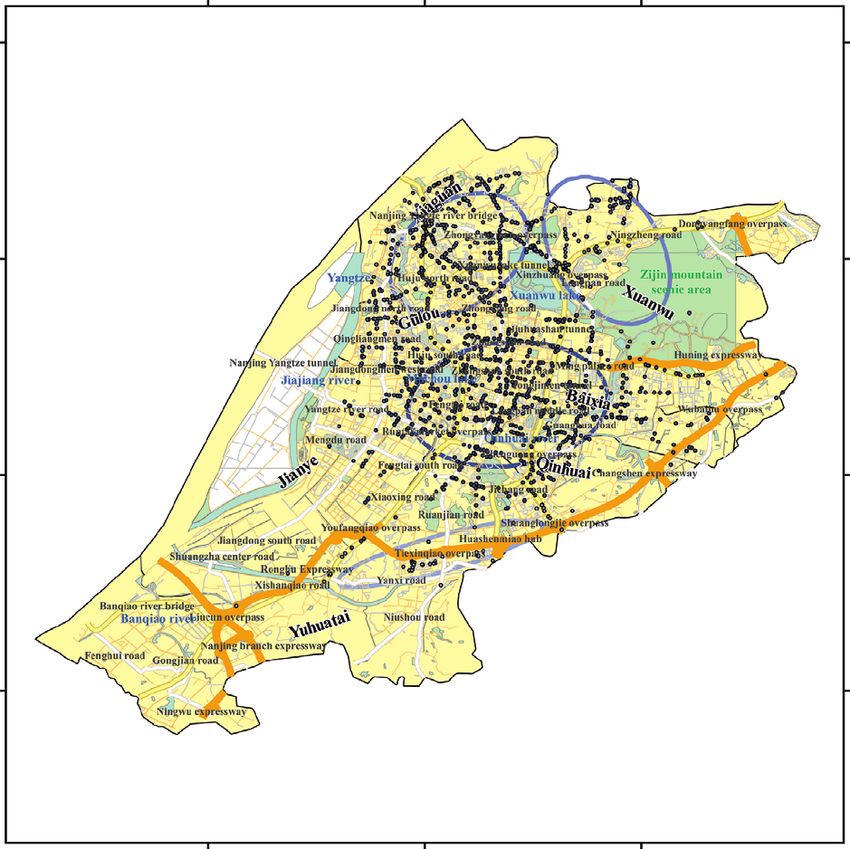
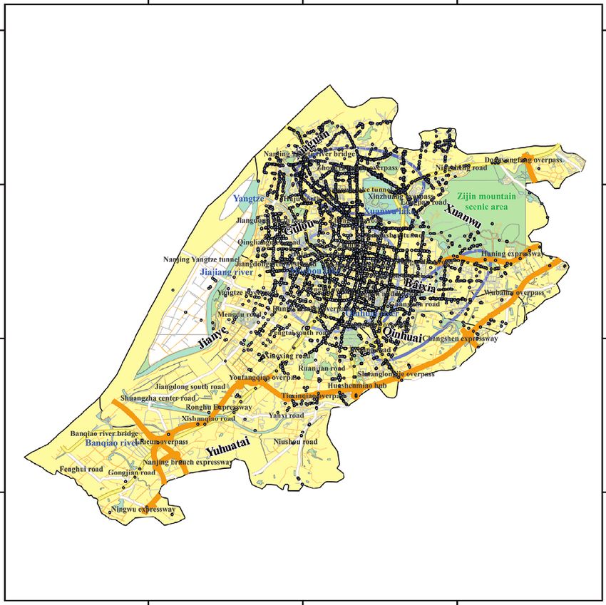
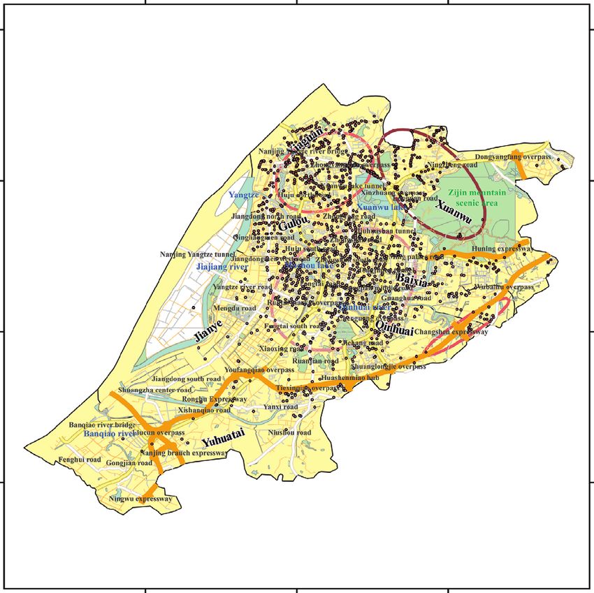
Journal of Advanced Transportation 9

 32°10′0″N 118°40′0″E 118°45′0″E 118°50′0″E 118°40′0″E 118°45′0″E 118°50′0″E

 32°10′0″N

 32°10′0″N

 32°10′0″N
 N N
 Community detection of origins Community detection of destinations
 from 22:00 to 23:00 from 22:00 to 23:00
 32°5′0″N

 32°5′0″N

 32°5′0″N

 32°5′0″N
 32°0′0″N

 32°0′0″N

 32°0′0″N

 32°0′0″N
 31°55′0″N

 31°55′0″N

 31°55′0″N

 31°55′0″N
 0 5 10 (km) 0 5 10 (km)

 118°40′0″E 118°45′0″E 118°50′0″E 118°40′0″E 118°45′0″E 118°50′0″E

 Origins Taxi pick-up community Destinations Taxi drop-off community
 Origins in no.1 community No.1 community Destinations in no.1 community No.1 community
 Origins in no.2 community No.2 community Destinations in no.2 community No.2 community
 Origins in no.3 community No.3 community Destinations in no.3 community No.3 community
 Origins in no.4 community No.4 community Destinations in no.4 community No.4 community
 Origins in no.5 community No.5 community Destinations in no.5 community No.5 community
 Origins in no.6 community No.6 community Destinations in no.6 community No.6 community
 (d)

Figure 7: (a) Community detection results of origin and destination from 8 : 00 to 9 : 00. (b) Community detection results of origin and
destination from 13 : 00 to 14 : 00. (c) Community detection results of origin and destination from 18 : 00 to 19 : 00. (d) Community detection
result of origin and destination from 22 : 00 to 23 : 00.

spatial clustering, and differences between different Community No. 4, and the drop-off points of the decile
communities. before the visit were mostly distributed in Community No. 1:
 In summary, the characteristics of the passenger travel in the southeast of Gulou, southwest of Xuanwu, west of
activity time distribution show more daytime and fewer Qinhuai, northeast of Jianye, and north of Yuhuatai. These
nighttime activities and frequent peak hours in the morning are adjacent areas of the main urban centers, and the pick-up
and evening. The characteristics of the passenger travel or drop-off points in the decile after the visit heat and the
activity spatial distribution show concentrated urban centers visit heat were randomly distributed. Therefore, it can be
and scattered peripheral areas. Affected by the purpose of concluded that passenger travel hot spots were clustered or
travel and structure of the community, passenger travel dispersed as passenger travel activity increased or decreased.
activities behave in the same way in the same community at Xu et al. [19] showed that the hot spots in Nanjing have a
the same time, and there is an interaction between different spatial distribution characteristic of clustering from the
communities at the same time. surroundings to the center and that Moran’s I value around
 the clustering center is negative. The hot spots of passenger
4.2. Passenger Travel Hot Spot Analysis. Taking the 8 : 00–9: travel extracted in this study are consistent with the results of
00 time period as an example, we considered the minimum the previous study, and a more obvious spatial local ag-
circle radius of the community, including the pick-up and glomeration can be found based on community detection of
drop-off points, as the aggregation distance, and the out- pick-up and drop-off points.
bound visit heat and arrival visit heat of the passenger’s Taking the period from 8 : 00 to 9 : 00 as an example, the
travel activity as the indicators. The corresponding com- average visit heat and average visit heat statistics were
munities were divided according to the first decile, and the calculated on five graded road sections: national highway,
pick-up and drop-off points were aggregated to extract hot provincial highway, county highway, township and village
spots. Furthermore, the pick-up and drop-off points in the highway, and other roads, as shown in Table 1.
corresponding community were aggregated according to the It can be seen from Table 1 that the average visit pop-
last decile to extract cold spots, as shown in Figure 8. ularity ordered from high to low was township and village
 It can be clearly observed from Figure 8 that the pick-up roads, provincial roads, other roads, county roads, and
points of the decile before the visit were distributed in national roads. The average visit popularity ordered from
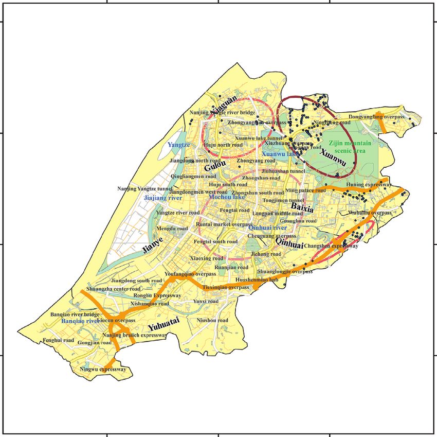
10 Journal of Advanced Transportation

 32°10′0″N 118°40′0″E 118°45′0″E 118°50′0″E 118°40′0″E 118°45′0″E 118°50′0″E

 32°10′0″N

 32°10′0″N

 32°10′0″N
 N N
 Cold spots of origins in taxi pick-up Hot spots of origins in taxi pick-up
 communities from 8:00 to 9:00 communities from 8:00 to 9:00
 32°5′0″N

 32°5′0″N

 32°5′0″N

 32°5′0″N
 32°0′0″N

 32°0′0″N

 32°0′0″N

 32°0′0″N
 31°55′0″N

 31°55′0″N

 31°55′0″N

 31°55′0″N
 0 5 10 (km) 0 5 10 (km)

 118°40′0″E 118°45′0″E 118°50′0″E 118°40′0″E 118°45′0″E 118°50′0″E

 Cold spots of origins value of departure: Hot spots of origins value of departure:

 [0.050896, 0.085807] [0.730182, 0.80000]
 Taxi pick-up communities Taxi pick-up communities
 No.1 community No.1 community
 No.2 community No.2 community
 No.3 community No.3 community
 No.4 community No.4 community
 (a)
 118°40′0″E 118°45′0″E 118°50′0″E 118°40′0″E 118°45′0″E 118°50′0″E
 32°10′0″N

 32°10′0″N

 32°10′0″N

 32°10′0″N
 N N
 Cold spots of destinations in taxi drop-off Hot spots of destinations in Taxi drop-off
 communities from 8:00 to 9:00 communities from 8:00 to 9:00
 32°5′0″N

 32°5′0″N

 32°5′0″N

 32°5′0″N
 32°0′0″N

 32°0′0″N

 32°0′0″N

 32°0′0″N
 31°55′0″N

 31°55′0″N

 31°55′0″N

 31°55′0″N

 0 5 10 (km) 0 5 10 (km)

 118°40′0″E 118°45′0″E 118°50′0″E 118°40′0″E 118°45′0″E 118°50′0″E

 Cold spots of destinations value of arrival: Hot spots of destinations value of arrival:

 [0.039249, 0.075679] [0.734238, 0.80786]
 Taxi drop-off communities Taxi drop-off communities
 No.1 community No.1 community
 No.2 community No.2 community
 No.3 community No.3 community
 No.4 community No.4 community
 (b)

Figure 8: (a) Hot and cold spots of origins in pick-up communities from 8 : 00 to 9 : 00. (b) Hot and cold spots of destinations in drop-off
communities from 8 : 00 to 9 : 00.
Journal of Advanced Transportation 11

 Table 1: Average activity of graded roads.
Graded road Number of roads Average value of departure Average value of arrival
National roads 66 0.530 0.598
Provincial roads 84 0.648 0.474
County roads 181 0.594 0.546
Township and village roads 1191 0.694 0.582
Other roads 178 0.626 0.592

high to low was national roads, other roads, town and village was Sun Ye Village, corresponding to Longzang Avenue.
roads, county roads, and provincial roads. This shows that passenger travel activities were closely re-
 By searching the database, we found that the represen- lated to the zoning functions carried by land use types.
tative road sections with higher outbound visits on the graded A study by Jin and Xu [21] showed that the inflow and
roads were Yurun Street, Fengqi Road, Jiajiang Bridge, Jin- outflow on the key nodes of Nanjing’s road network of
su’an Road, and Caodu Lane; representative sections with different levels have an obvious hierarchical structure, and
lower outbound visits were Fengwu Road, Binjiang Road, different points of interest play a certain role in the flow of
Jiangshan Street, Chuanjiang Street, and Houde Road. Rep- tourists. The results of passenger travel activity at different
resentative road sections with higher arrival visits were points of interest in our study were consistent with the
Zhenxing Road, Shuangtang Road, Jiangshan Street, Xiao- conclusions of the previous research.
fenqiao, and Fanjiatang. Representative sections with lower In summary, urban roads contain information about the
arrival visits were Fengwu Road, Moxiang Road Overpass, classification functions of expressways, arterial roads, sec-
Nanjing Yangtze River Tunnel, Lingyin Road, and Kuitou ondary arterial roads, and branch roads and are affected by
Alley. This shows that passenger travel activities are closely land use types. The pick-up and drop-off points with high
related to the traffic functions carried by the graded roads. The passenger travel activity were concentrated near points of
main function of expressways is to enable continuous traffic, interest, forming hot spots. On the contrary, the pick-up and
of trunk roads is to enable transportation, of secondary trunk drop-off points with low passenger travel activity were
roads is to enable distribution traffic, and of branch roads is to concentrated near points of interest, and cold spots were
enable service in local areas. formed. The hot spots of outbound visits were scattered on
 A study by Yang [20] showed that there is cascading urban residential land, and the hot spots of arrival visits were
failure and congestion in the traffic system of Nanjing. Travel concentrated on commercial and financial land.
conditions of people in an unbalanced road network load are
affected by the coupling of sub-road networks. The results of
passenger travel activity on graded roads in this study are 5. Comparison and Discussion
consistent with the conclusions of that research.
 Taking the 8 : 00–9:00 period as an example, based on the 5.1. Comparison. The GN algorithm [16] includes a splitting
residents’ walking considerations, the pick-up and drop-off algorithm that uses the number of shortest paths passing
points are the center of the circle with a radius of 300 m for through each edge in the network as a measurement index,
coverage, covering commercial land, residential land, public and gradually deletes edges that do not belong to any
management and public service land, and transportation community. Newman’s fast algorithm [17] uses a cohesive
land. The average outbound visit heat and average arrival algorithm, starting with each node occupying a community
visit heat were calculated for approximately 30 types of land and continuously merging in the direction that maximizes
use involving a total of 26,000 points of interest, as shown in the increase in modularity. Compared with the GN algo-
Table 2. rithm and the Newman fast algorithm, we use Bayes’ rule to
 It can be seen from Table 2 that the land use type with the set the weight of the edge betweenness of the network, and
highest average outbound visit heat was urban residential the heap data structure to calculate the modularity; we also
land, and the land use type with the lowest average outbound reduce the complexity of the algorithm and use the standard
visit heat was commercial and financial land. The land use deviation ellipse to make the detected community structure
type with the highest average arrival visit heat was com- clearer. For a complex network with n nodes and m con-
mercial and financial land. The lowest average arrival visited necting edges, the comparison results of the GN algorithm,
land use type was urban residential land. Newman fast algorithm, and the algorithm in this paper are
 By searching the database, the representative point of listed in Table 3.
interest with higher average outbound visits was Yangz- Theoretically, if there are n communities, an n × n
huang Village, corresponding to Shiyang Road. The repre- symmetric matrix F can be defined. The trace of the matrix
sentative point of interest with lower average outbound visits (the sum of the diagonal elements of the matrix) is
was Flower Building, corresponding to Software Avenue. Tr(F) � fii , which means the ratio of all edges connecting
The representative point of interest with higher average the nodesi within the community to the total number of
arrival visits was Commercial Century Plaza, corresponding edges in the network. Tr(F) value is in the range of [0, 1]. It
to the Xinjiekou commercial pedestrian area. The repre- is used to calculate modularity, and to a certain extent also
sentative point of interest with lower average arrival visits characterizes the complexity of the network structure.
12 Journal of Advanced Transportation

 Table 2: Activities at different points of interests.
 Land use types Interests Total Value of departure Value of arrival
 Retail land Shopping malls, supermarkets, etc. 4381 0.722 0.578
 Dining land Hotels, restaurants, etc. 5210 0.700 0.568
Commercial
 Financial land Office buildings, financial centers, etc. 462 0.276 0.648
 Other land Banks, business halls, etc. 2284 0.738 0.590
Residential Residential land Apartments, villas, etc. 2161 0.790 0.288
 Agency land Government agencies, etc. 810 0.674 0.574
 Education land Schools, institutes, etc. 1376 0.614 0.508
Public
 Medical land Hospitals, pharmacies, etc. 1881 0.660 0.540
 Green land Parks, gardens, etc. 74 0.554 0.450
 Street land Parking lot, transportation station, etc. 324 0.700 0.576
Traffic
 Highway land Toll station, bus station, etc. 7206 0.308 0.444

 Table 3: Method comparison.
Characteristic GN algorithm Newman fast algorithm Algorithm of this paper
Algorithm complexity O(nm2 ) O(n2 ) O(mlog2 n)
Number of communities Unknowable Knowable Knowable
Community structure No overlap Overlap Overlap

 When the network structure is abnormally chaotic, there 1
are fewer edges connecting nodes within the community, and 0.95
 Community detection

 0.90
the value of Tr(F) is minute. When the network structure is 0.85
 accuracy

abnormally single, there are excessive number of edges 0.80
connecting the nodes within the community, and the value of 0.75
 0.70
Tr(F) is extremely large. When Tr(F) value is in the range of 0.65
[0.4, 0.6], it can be assumed that the network structure is 0.60
normal and that the value is not an abnormal value. 0.55
 Therefore, another way of expressing modularity is 0.50
 0 0.2 0.4 0.6 0.8 1
M � Tr(F) − F2 , and F2 is the modulus of matrix F2 . We Tr(F)
compare the accuracy of community detection models using
the GN algorithm, Newman fast algorithm, and the algo- GN algorithm
rithm in this paper, as shown in Figure 9. Newman fast algorithm
 Algorithm of this paper
 The community detection algorithm centered on the
hierarchical structure is divided into split and aggregation Figure 9: Algorithm performance comparison chart.
types. The GN algorithm belongs to the split type, and the
Newman fast algorithm and the algorithm proposed in this unconnected communities are merged, the degree of
article belong to the aggregation type. modularity remains unchanged; thus, the communities that
 The GN algorithm gradually deletes edges that do not are connected by edges and the corresponding internal
belong to any community (i.e., the edges connected between nodes can be divided more accurately.
communities) according to the degree to which the edges do As shown in Figure 9, the abscissa is Tr(F) and the
not belong to the community, until all edges are deleted. ordinate represents the accuracy of community detection.
Because the edge betweenness of each connected edge needs The circle is the GN algorithm, the triangle is the Newman
to be recalculated every time an edge is removed, for complex fast algorithm, and the square is the algorithm used in this
network structures, the algorithm can be easily implemented study. It can be clearly observed from the figure that the
by splitting it across more independent communities. accuracy of the algorithm in this study is significantly higher
 Newman’s fast algorithm starts with each node occu- than that of the GN algorithm. Compared with the Newman
pying a community and continues to merge communities in fast algorithm, when Tr(F) is [0, 0.2], [0.4, 0.6], and [0.8, 1],
the direction that maximizes the increase in modularity until the algorithm used in this study has higher accuracy.
the entire network merges into one community. Because the Therefore, according to Figure 9 and Table 3, the accuracy of
modularity needs to be increased every time the commu- the algorithm in this study is equivalent to that of the
nities connected by edges are merged, when the network Newman fast algorithm, but the running time is faster, and
structure is simple, the execution of this algorithm will easily thus the performance is better.
lead to the incorrect division of nodes. This demonstrates that when the network structure is
 The algorithm proposed in this paper introduces Bayes’ abnormally single or chaotic, the community detection
rule and takes the amount of information as the increment of model using the algorithm proposed in this study can
modularity, without calculating the adjacency matrix to discover more complex community structures and has better
ensure the increment of modularity. Therefore, when interpretability for community detection results.
Journal of Advanced Transportation 13

 Degree distribution Qin et al. [18] analyzed the intensity of node access degrees
 0.15 0.14 and edge weights based on the network interaction of urban
 0.135 0.1375 N = 4870 hot spots, without considering the potential impact of land use
 p = 0.0017
 0.12 0.12 on urban residents’ travel decisions. This study combined the
 0.115
 hierarchical road network and point of interest data to explore
 hot spots from the perspective of individual taxi passengers
 0.09 0.09 interacting with the community, which helped to explore the
 0.0775
 P(k)

 formation process of urban hot spots.
 0.06
 0.05 6. Conclusions
 0.0375 0.035
 0.03 This study extracted the passenger pick-up and drop-off
 0.02 0.0225 points from taxi movement trajectory data, constructed a
 0.01 0.01 taxi passenger travel activity index based on community
 0 2 4 6 8 10 12 14 16
 detection, and extracted the hot spots of taxi passenger travel
 k
 in the main urban area of Nanjing. The following three
 conclusions were drawn:
 Figure 10: Degree distribution of the model.
 (1) The travel activities of taxi passengers showed a time
 distribution pattern of more daytime, less nighttime,
 0.1
 and frequent morning and evening peak hours.
 0.94
 0.90 Affected by the purpose of travel, the degree of
 0.9 0.88
 Community detection accuracy

 community modularity and anisotropy rate of taxi
 0.8 0.74 0.80 0.74
 0.72
 passengers’ pick-up and drop-off points were posi-
 0.7
 0.63 0.63 tively correlated during morning and evening peak
 0.6 0.60 0.57 hours and negatively correlated during other
 0.53
 0.5 0.44 0.51 periods.
 0.4 0.43
 0.34 0.39 0.35 (2) The travel activities of taxi passengers presented a
 0.3 spatial distribution pattern, in which the central area
 0.28 0.28
 0.2 of the city was concentrated and the outer areas were
 0.1 0.14 scattered. Affected by the structure of the commu-
 0 nity, passenger travel activities showed a consistent
 1 2 3 4 5 6 7 8
 behavioral pattern within the community and had
 Number of communities
 obvious spatial gathering characteristics. Further-
 Figure 11: Box plot of model parameter sensitivity analysis. more, there was a significant interaction between
 different communities.
5.2. Discussion. In order to explore the parameter sensitivity (3) The hot spots for taxi passengers’ travel were scattered
of the community detection model in this study, taking the on urban residential land and concentrated on com-
period of 8 : 00–9:00 as an example, the degree distribution mercial and financial land. Affected by land use,
of the random network was calculated, as shown in Fig- passenger travel activity indicators were closely related
ure 10, and 21 simulation experiments were performed to to road grades and types of points of interest. Pas-
compare the accuracy, as shown in Figure 11. senger travel hot spots were clustered as activity levels
 As shown in Figure 10, the abscissa represents the degree increased and dispersed as activity levels decreased.
of the node, the ordinate represents the degree distribution Subsequent research needs to consider more sources of
probability, N represents the number of nodes, and p data, such as combining rental car trajectory data with bus
represents the connection probability of the nodes. It can be trajectory data, analyzing the travel preferences of different
clearly observed from Figure 10 that the average degree of groups of people, and further exploring the temporal and
the node is eight, and the degree distribution follows the spatial patterns of urban traffic congestion by urban resi-
Poisson distribution. dents using the impact of different travel modes.
 As shown in Figure 11, the abscissa represents the
number of communities, and the ordinate represents the
accuracy of community detection. It can be clearly observed
 Data Availability
from Figure 11 that when the number of communities All data, models, and code that support the findings of this
detected is four, the accuracy reaches its peak. study are available from the corresponding author upon
 In summary, in a random network composed of 4870 key reasonable request.
road network nodes, different communities are delineated
based on taxi passengers’ pick-up and drop-off points within Conflicts of Interest
a representative period, and the detected travel hot spots
have reasonable spatial distribution characteristics. The authors declare that they have no conflicts of interest.
14 Journal of Advanced Transportation

Authors’ Contributions coarse-graining,” Scientific Reports, vol. 9, no. 1, pp. 1–10,
 2019.
Yuyu Sheng, Shuoben Bi, and Wenwu He conceived and [14] Yu Zheng, Y. Liu, J. Yuan et al., “Urban computing with
designed the experiments; Yuyu Sheng and Ruizhang Xu taxicabs,” in Proceedings of the 13th International Conference
performed the experiments; Yuyu Sheng, Shuoben Bi, and on Ubiquitous Computing - UbiComp’11, pp. 89–98, ACM,
Ruizhuang Xu wrote the Chinese paper; Shuoben Bi and Beijing, China, 2011.
 [15] R. L. Wu, X. Y. Zhu, and W. Guo, “Spatiotemporal distri-
Jingjing Fan translated the paper.
 bution patterns of urban road traffic accidents,” Geomatics &
 Spatial Information Technology, vol. 41, no. 07, pp. 103–106,
Acknowledgments 2018.
 [16] M. Gong and M. Girvan, “Finding and evaluating community
This work was supported by the National Natural Science structure in networks,” Physical Review E Statistical Nonlinear
Foundation of China (Grants: 41971340 and 41271410). & Soft Matter Physics, vol. 69, no. 2, pp. 26113–26120, 2004.
 [17] M. E. J. Newman, “Fast algorithm for detecting community
 structure in networks,” Physical Review E, vol. 69, no. 6,
References Article ID 066133, 2004.
 [18] K. Qin, Q. Zhou, Y. Q. Xu et al., “Spatial interaction network
 [1] Q. Q. Li and D. R. Li, “Big data GIS,” Geomatics and Infor- analysis of urban traffic hotspots,” Progress in Geography,
 mation Science of Wuhan University, vol. 39, no. 06, vol. 36, no. 9, pp. 1149–1157, 2017.
 pp. 641–644, 2014. [19] J. Xu, S. B. Bi, Y. Zhang et al., “PSO⁃SVM model based analysis
 [2] Y. Zheng, “Introduction to urban computing,” vol. 40, no. 01, on traffic flow of road intersections in Nanjing,” Modern
 , pp. 1–13, Geomatics and Information Science of Wuhan Electronics Technique, vol. 39, no. 17, pp. 128–213, 2016.
 University, 2015. [20] X. X. Yang, “On the Model and Congestion Performance of
 [3] Y. Liu, X. Liu, S. Gao et al., “Social sensing: a new approach to Nanjing Urban Public Traffic Systems,” Nanjing University of
 understanding our socioeconomic environments,” Annals of Posts and Telecommunications, 2018.
 the Association of American Geographers, vol. 105, no. 3, [21] C. Jin and J. Xu, “Study on the tourists flow among external
 pp. 512–530, 2015. transport nodes and hotels in Nanjing,” Human Geography,
 [4] J. M. Harvey and J. W. Han, Geographic Data Mining and vol. 31, no. 05, pp. 55–62, 2016.
 Knowledge Discovery, CRC Press, London, UK, 2009. [22] L. Zhao, M. Deng, D. L. Peng et al., “Structural property
 [5] C. X. Cheng, P. J. Shi, C. Q. Song et al., “Geographic big-data: analysis of urban Street networks based on complex network
 anew opportunity for geography complexity study,” Acta theory,” Geography and Geo-Information Science, vol. 26,
 Geographica Sinica, vol. 73, no. 08, pp. 1397–1406, 2018. no. 05, pp. 11–15, 2010.
 [6] M. Veloso, S. Phithakkitnukoon, and C. Bento, “Urban [23] G. N. Wang, Spatial-Temporal Data Mining Based on GPS
 mobility study using taxi traces,” in Proceedings of the 2011 Trajectory and Geo-Tagged Photo Trajectory, Central South
 International Workshop on Trajectory Data Mining and University, Changsha, China, 2013.
 Analysis – TDMA’11, pp. 23–30, ACM, New York, NY, USA, [24] S. Z. Guo and Z. M. Lu, The Basic Theory of Complex Network,
 2011. Science Press, Beijing, China, 2012.
 [7] R. Ahas, A. Aasa, Y. Yuan et al., “Everyday space-time ge- [25] Y. Batty, Study on Human Activity Space Patterns and Net-
 ographies: using mobile phone-based sensor data to monitor work Spatial Temporal Characteristics in Urban Cities Using
 urban activity in Harbin, Paris, and Tallinn,” International Taxi Trajectory Data, Wuhan University, Wuhan, China,
 Journal of Geographical Information Science, vol. 29, no. 11, 2016.
 pp. 2017–2039, 2015. [26] Y. L. An, Z. F. Huang, W. D. Chen et al., “Spatial evolution of
 [8] R. W. Scholz and Y. Lu, “Detection of dynamic activity county economy in Anhui Province during 2001-2010,”
 patterns at a collective level from large-volume trajectory Progress in Geography, vol. 32, no. 05, pp. 831–839, 2013.
 data,” International Journal of Geographical Information
 Science, vol. 28, no. 5, pp. 946–963, 2014.
 [9] J. Cui, F. Liu, D. Janssens, G. Wets, and M. Cools, “Detecting
 urban road network accessibility problems using taxi GPS
 data,” Journal of Transport Geography, vol. 51, no. 12,
 pp. 147–157, 2016.
[10] C. Zhong, S. M. Arisona, X. Huang, B. Michael, and
 G. Schmitt, “Detecting the dynamics of urban structure
 through spatial network analysis,” International Journal of
 Geographical Information Science, vol. 28, no. 11, pp. 2178–
 2199, 2014.
[11] Q. Huang, Y. Yang, Z. Yuan et al., “The temporal geo-
 graphically-explicit network of public transport in Chang-
 chun City, Northeast China,” Scientific Data, vol. 6,
 no. 190026, pp. 1–10, 2019.
[12] F. Guo, D. Zhang, Y. Dong et al., “Urban link travel speed
 dataset from a megacity road network,” Scientific Data, vol. 6,
 no. 61, pp. 1–8, 2019.
[13] H. Hamedmoghadam, M. Ramezani, and M. Saberi, “Re-
 vealing latent characteristics of mobility networks with
You can also read