Opening up the court: analyzing player performance across tennis Grand Slams

JQAS 2021; aop

JQAS

Shannon K. Gallagher*, Kayla Frisoli, and Amanda Luby
Opening up the court: analyzing player
performance across tennis Grand Slams

Abstract: In tennis, the Australian Open, French Open, Wimbledon, and US Open
are the four most prestigious events (Grand Slams). These four Grand Slams
differ in the composition of the court surfaces, when they are played in the year,
and which city hosts the players. Individual Grand Slams come with different
expectations, and it is often thought that some players achieve better results at
some Grand Slams than others. It is also thought that differences in results may
be attributed, at least partially, to surface type of the courts. For example, Rafael
Nadal, Roger Federer, and Serena Williams have achieved their best results on
clay, grass, and hard courts, respectively. This paper explores differences among
Grand Slams, while adjusting for confounders such as tour, competitor strength,
and player attributes. More specifically, we examine the effect of the Grand Slam
on player performance for matches from 2013-2019. We take two approaches to
modeling these data: (1) a mixed-effects model accounting for both player and
tournament features and (2) models that emphasize individual performance. We
identify differences across the Grand Slams at both the tournament and individual
player level.

Keywords: tennis; hierarchical modeling; mixed-effects model; open-source; re-
producible research

1 Introduction
The four tennis Grand Slams (Australian Open (AO), French Open (FO), Wim-
bledon (Wim.), US Open (USO)) are played in different cities (Melbourne, Paris,
London, New York City) at different times of the year (January, May, June/July,
August/September) They are played over the course of two weeks with seven total

*Corresponding author: Shannon K. Gallagher, Dept. of Statistics & Data Science,
Carnegie Mellon University
Kayla Frisoli, Dept. of Statistics & Data Science, Carnegie Mellon University
Amanda Luby, Dept. of Mathematics and Statistics, Swarthmore College

2 Gallagher, Frisoli, and Luby

rounds and 128 players in both the men’s (ATP) and women’s (WTA) tours. All
four slams are played on different surfaces (Plexicushion hard court, clay, grass,
DecoTurf hard court), and it is commonly thought that top players perform better
at certain slams. For instance, Spanish players, led by Rafael Nadal, seem to have
dominated the French Open in recent years (Lewit, 2018). In addition, “home court
advantage” is believed to play a role, in which players from the country of the
Grand Slam tournament are thought to perform better at home than at other
Grand Slams.
 In this paper, we use 2013-2019 tennis data to analyze differences in player
performance at Grand Slams. We highlight three players to motivate our interest
in performance across different slams. Nadal is known as the “King of Clay” in
tennis, having won 13 out of his current 20 Grand Slams titles at the French Open
(Jurejko, 2018). In contrast, Nadal’s rival Roger Federer has won most of his Grand
Slam titles (8 out of 20) at Wimbledon. On the women’s side, Serena Williams,
winner of 23 Grand Slam titles, has been dominant both on hard court (7 titles at
the Australian Open and 6 at US Open) and grass (7 at Wimbledon). This is not to
imply that other successful players such as Djokovic, V. Williams, and Sharapova
are irrelevant in the study of Grand Slam effects, but in this paper we use Nadal,
Federer, and S. Williams as the prime examples of slam-specific dominance.
 Existing literature provides methods for forecasting the outcome of tennis
matches (Klaassen and Magnus, 2003; Newton and Keller, 2005; McHale and
Morton, 2011; Kovalchik, 2016) and for assessing whether points within a match
are independent and identically distributed (Klaassen and Magnus, 2001). Barnett
and Pollard (2007); Paxinos (2007); Knottenbelt et al. (2012); Sipko (2015) look
into building models that take the court surface / tournament into account. Results
from studies performed in other sports show that surface type does have an effect
on the game, either directly or indirectly (Andersson et al., 2008; Gains et al.,
2010). There also have been a number of papers about specific players including
Federer, S. Wiliams, and Nadal with regards to performance prediction and other
modeling (Newton and Aslam, 2009; Leitner et al., 2009; Morris, 2015; Wei et al.,
2013).
 We examine the impact of tournament on performance across all participants
in Grand Slams, and also investigate the impact on individual players, with a focus
on Nadal, Federer, and S. Williams. To analyze the differences, we
1. Perform exploratory data analysis to visualize and understand the data at a
 high level and assess commonly held beliefs about player performance at the
 four Grand Slams.
2. Develop general mixed-effects models to estimate effects of some variables,
 such as rank and opponent rank, that are constant across all players, while
 capturing individual effects across each player for each slam.

Opening up the court 3

3. Model players individually to assess specific strengths and weaknesses across
 the Grand Slams.

Our first approach is to explore how specific attributes of our data change across
slams using visualizations. We examine the distribution of total points, wins, aces
(a serve an opponent is unable to return), and unforced errors (UE) (when a player
makes a simple mistake resulting in a loss of the point) across tournaments. In this
expoloratory analysis, we do not find evidence in favor of a home-court advantage
and only find little evidence suggesting that Spanish players perform better on clay
(i.e., at the French Open). We confirm the well-known claim that taller players are
better servers (regardless of slam).
 Our second approach is to develop a general mixed-effects regression model
(also called a hierarchical model), which takes into account player and tournament
attributes. We use data that includes all Grand Slam matches from 2013-2019. A
mixed-effects modeling approach leverages tournament information from all players,
allowing us to model players with few matches played. This approach, furthermore,
accounts for the same players appearing multiple times in the data, since players
may participate in multiple Grand Slams each year, resulting in non-independent
observations. We are thus able to simultaneously analyze player and slam effects.
 Our third approach is to model performance for specific players individually,
with subsets of the data set that provide detailed point-by-point information for
top players. We look at the top 10 WTA and ATP players, based on the total
number of Grand Slam matches played between 2013 and 2019.
 To validate our conclusions, we use common model fit measures such as AIC.
We also examine whether our models pass “common sense” tests (e.g., how the
models in Thomas et al. (2013) show that commonly well known hockey players
also have high status in the model). Further, we examine whether specific tennis
players perform better at different slams. All of our data used in this analysis is
open source and described in detail in Section 2. Moreover, all methods and models
are reproducible and available online (details in Section 2.1).
 The rest of this paper is organized as follows. In Section 2, we describe the
Grand Slam tennis data and examine it at a high level (Approach 1). In Section 3.1,
we describe our general mixed-effects models and results (Approach 2). In Section
3.2, we describe our approach to creating individual models for each player and
provide a summary of results (Approach 3). Finally, Section 4 provides a summary
of all results and discusses future work.

4 Gallagher, Frisoli, and Luby

2 Data and exploratory data analysis
2.1 Data

All data in our analysis is obtained via the R package deuce (Kovalchik, 2017),
which accesses repositories of Sackmann (2021) containing data from the four
Grand Slam websites. The complete Grand Slams data set consists of 7112 matches
split evenly over the seven rounds of each of the four Grand Slams (2013-2019) for
the two tours: ATP (men’s) and WTA (women’s). Each match has 80 attributes,
many of which are redundant. We focus on the following attributes for both the
winner and loser of the match: games won, points won, retirement, break points
faced, break points saved, aces, country of origin, and player attributes such as
age, height, and weight. Additionally, we take into account the number of sets in a
match, and the round of the tournament. Note that in Grand Slams, men play a
best of five set match, and the women a best of three. An example of the data is
shown in Table 1.
 The secondary data set originated as partial point-by-point data for Grand
Slam matches. In this data set, each row is a point in a match with details on who
won the point, service speed, and whether a player had a forced or unforced error,
winner, ace, or net point win. There is also tournament information such as court
surface, year, and time start. Additional attributes include rally length, winner and
final score of the match, retirement, and minutes played. However, these additional
attributes are only available for a subset of the matches recorded in the primary
data set. After aggregating the point-by-point data over the match, this partial data
set consists of 3858 observations (compared to the 7112 matches in the primary
data set). An example of the data is shown in Table 2.
 Across both the ATP and WTA, the median rank of the winners for the primary
data is 29, and the median rank for the winners of the secondary data is 22. The
median rank among losers in the secondary dataset is also higher than the primary.
This indicates that better-ranked (lower) players are more likely to have point by
point data recorded, which indicates that the missing data in the secondary, partial
data is not random. Additionally, we find that no WTA point-by-point data are
available for 2015. Finally, there are no point-by-point data for 2018-2019 at both
the French Open and the Australian Open.
 In Table 3, we display the number of matches Nadal, Federer, and S. Williams
played from 2013-2019 at the four Grand Slams. Over that time span, Nadal won
eight Grand Slams, Federer won three, and S. Williams won eight. Of these three,
Federer has played the most matches at Wimbledon (41), Nadal at the French
Open (43), and Williams the most on hardcourts (75 between the US Open and

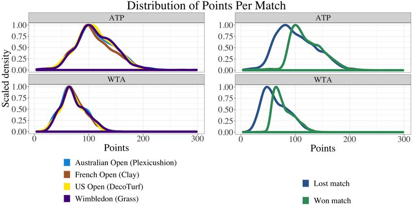
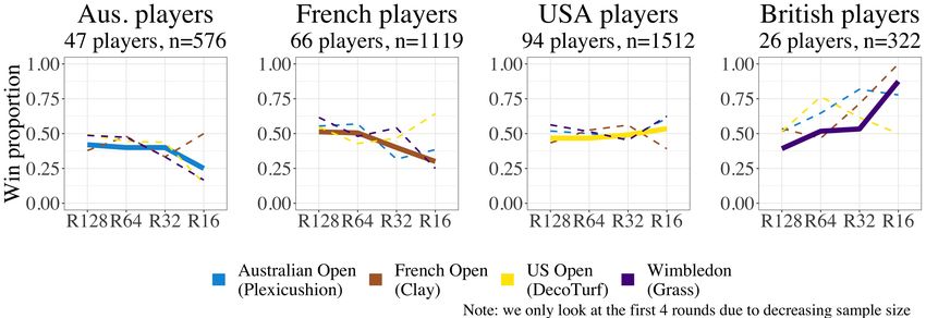
Opening up the court 5

Australian Open). Notably, these three players missed at least three slams each
due to external factors such as injury.

2.2 Distribution of points scored

We first examine whether the distribution of number of points per match differs
by slam in Figure 1 (left), while accounting for the tour (ATP vs. WTA). This
distribution is similar across tournaments, with Wimbledon differing slightly from
the other Grand Slams. As expected, there are more points scored in the ATP
than the WTA (Figure 1 (right)) due to the differing number of sets played. Also
unsurprisingly, the winners of the match tend to score more points than the losers.
However, about 5% of players who won the match actually scored fewer points
than their opponent, and not all of these can be attributed to player retirement.

2.3 Home court advantage

It is commonly thought that there is a home court advantage in Grand Slam
matches (Morris, 2013). For example, we may expect French players to achieve
better results at the French Open compared to the other slams. However, the host
city is given preference for wild card bids (USTA, 2018) so potentially citizens of a
given country play in their “home” tournament more often than they play in other
tournaments. The data confirms this notion, e.g., the proportion of French players
in the French Open is greater than the proportion of French players in other slams.
 We explore how the proportion of wins for the home country changes across the
different tournaments. If there really is a home court advantage, after adjusting for
the ranking of players, the proportion of French wins each round would be higher
at the FO than the AO, the USO, and Wim.. The same would be true for Australia,
the US, and the UK. However, in Figure 2, this is not the case. We plot the percent
of matches won for the first four rounds for players of the four countries across
the four different Grand Slams. After accounting for the number of players from
each country, we do not find a statistically significant home court advantage in the
Grand Slams as the lines and their confidence intervals (not shown) overlap. In
fact, we note in the first round (R128) that the “home” players are typically losing
more than at other slams, which may indicate that adding more home players with
the wild card bid does not guarantee that those players will make it to later rounds.
In the subtitles of Figure 2 we note the number of players from each country (n),
which varies across the four countries. The varying sizes impact the variability

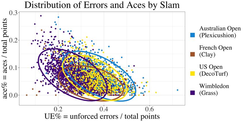
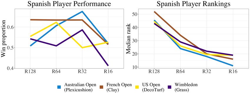
6 Gallagher, Frisoli, and Luby

of our results and are potentially why we see more pronounced differences in the
British players graph (which has the fewest players).
 While we include worse-ranked (i.e., higher rank) players who are able to
play courtesy of the wild-card bid, we can also exclude those and examine the
home-court advantage for players who typically play all four slams. We again find
that the results are not significant, but we do not display the results as they do
not differ from those in Figure 2. Regardless of whether we include wild-card bid
players from the home country or not, we do not find evidence of a home-court
advantage.

2.4 Spanish players at the French Open

Another common notion in tennis is that Spanish players perform better at the
French Open compared to the other slams. Most would agree this is true for Nadal,
but other players such as Muguruza, Ferrer, and Verdasco have also demonstrated
recent success on clay. This phenomenon may be explained by the fact that many
Spanish players grow up practicing on clay courts, which is typically less common
for players from other countries. We explore this phenomenon in Figure 3. It
appears that Spanish players win more often at the French Open in the first and
second rounds (R128 and R64, respectively), shown by the height of the brown line.
However, this result is not significantly higher ( -value = 0.219, 0.474 respectively)
using Chi-squared tests. We must also account for the ranking of the players at
each round, as having a median higher numerical rank (higher rank → worse player)
in later rounds indicates that the player is doing better than expected (we expect
to see better players in later rounds). When we explore the right graph of Figure 3,
the median ranking of Spanish players in the French Open is higher than other
tournaments within the first two rounds. In conclusion, we find that within the
initial two rounds, players from Spain in the French Open are worse in ranking yet
winning more often. Therefore, it is hard to tell from this data whether there is a
real effect and further analysis is needed to determine if Spanish players perform
better at the French Open.

2.5 Patterns in aces and unforced errors

In tennis, players strive to increase their number of aces and decrease their number
of unforced errors. We examine how this relationship differs by slam, given that
the serve is often considered to be the most important shot in tennis. In Figure 4
we plot the percentage of unforced errors and aces in a match and color each point

Opening up the court 7

by the slam. Matches in Wimbledon seem to follow different ace / unforced error
patterns than the other tournaments. These matches tend to cluster in the left
(and slightly upper) part of the graph, meaning that Wimbledon matches tend to
have fewer unforced errors and more aces. It is thought that the ball moves faster
on grass courts and so the larger number of aces is expected but making fewer
errors is surprising, especially because players seldom practice on grass. However,
the classification of “forced” versus “unforced” errors is subjective, and Wimbledon
scoring officials have a reputation for generous score keeping (Perrotta and Bialik,
2013; Bialik, 2014). A second possible explanation for this is that the rally length
of Wimbledon points is shorter than the other slams, but we do not currently have
data to test this hypothesis.
 Another common notion about tennis is that taller players are better servers.
In Figure 5 we explore this notion, where each point represents one player. We
see a strong positive correlation between the median percent of aces per match
and height, confirming prior beliefs. This trend also follows if we were to use the
mean ace percentage or if we plotted all of the tournaments separately. Very tall
players such as Karlovic and Isner consistently have a large percent of aces. Federer
consistently has more aces than expected for his height whereas, generally, Nadal
has fewer aces than expected for his height and Murray has about the expected
number. For the women’s game, the trend also holds true. We see S. Williams
with an extremely large number of aces for her height, whereas V. Williams serves
slightly fewer than expected, on average, for her height during this time period.

3 Statistical models to analyze differences
In addition to exploring the differences among the slams descriptively, we also
take a model-based approach to analyze the differences. We explore whether player
performance varies across tennis Grand Slams and ask questions ranging from
a high-level (e.g., are some Grand Slams associated with more unforced errors
than others) to a player level (e.g., does Federer hit more aces at Wimbledon than
other Grand Slams). As previously mentioned, we use two data sets: the primary
data with fewer tennis attributes (see Table 1) and the secondary data which has
point-by-point data and player specific attributes (see Table 2).
 Because of these differences in scope, we do not build one model to answer
all questions. Instead, we take two general modeling approaches: 1) mixed-effects
models, using all available data, with both effects that are fixed across all players
and effects that are ‘random’ and allowed to vary for each player, and 2) models
trained on subsets of the partial (but rich) data for specific individual players that

8 Gallagher, Frisoli, and Luby

have ample data. Section 3.1 details the mixed-effects modeling approach, while
Section 3.2 details the individual modeling approach.

3.1 Mixed-effect models

The mixed-effects model approach allows for the sharing of information across
different players when estimating the effects of common covariates, while still
allowing for individual player variation in the random effects. Because players
participate in different slams across different years, players appear multiple times
in the data and the observations (matches) are not independent. Including a player-
level effect allows us to account for this dependence. It also provides a way to assess
individual player tendencies, while estimating some effects that are assumed to be
similar across all players.
 Due to the unique scoring of tennis matches, the total number of points won is
not a robust measure of player performance. For instance, players may score few
points in a match due to a poor performance (e.g., losing many games 40-15 or
40-0), but they may also score (relatively) few points if they win a short match
(e.g., winning straight sets 6-0, 6-0). Matches may also be more competitive than
the final score indicates due to the use of “deuce” scoring. Modeling the number
of points won is further complicated by the difference in match length for men
(best of 5 sets) and women (best of 3 sets). Furthermore, modeling wins with a
mixed-effects model did not result in noticeable differences among top players after
accounting for rank and opponent rank (see Appendix A.1 for further details).
Instead of using ‘win’ as the outcome variable, we model match statistics that
may be more sensitive to slam differences – aces, net points won, and unforced
errors – to see if individual differences among players at different Grand Slams are
detectable.

3.1.1 Modeling tennis-specific outcomes

We use a binomial likelihood for each of the three outcome variables, where

 ∼ Binomial( , )
 = logit−1 ( + [ ] ) (1)
 = .

 represents the number of aces, unforced errors, or net point won in each match
(depending on the model), is the total number of points played in that match,

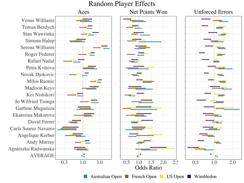
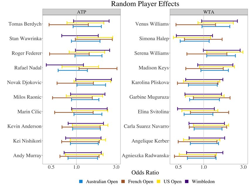
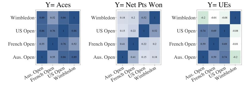
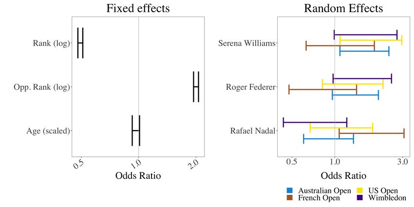
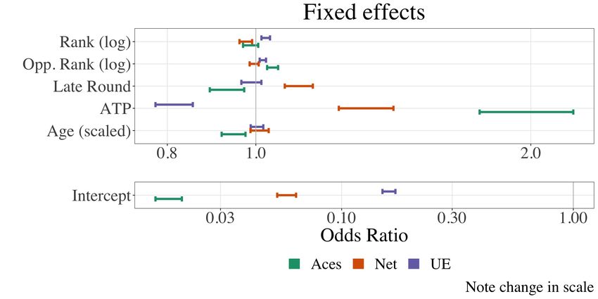
Opening up the court 9

 consists of indicator variables for the four Grand Slam tournaments, and 
includes an intercept, rank of player (log transformed), age of player (scaled), rank
of opposing player (log transformed), indicator variable for the ATP tour, and an
indicator variable for whether it was a late-round match. The feature “round of 16
or later” was used as a natural split because slams are structured such that the
first three rounds of matches occur during the first week and the next four during
the second week.
 Figure 6 shows the fixed effects coefficient estimates for each of the three
binomial models (Aces, Net Points (Net), Unforced Errors (UE)) on the odds
ratio scale. The regression coefficient tables are also displayed in Tables 4 - 6. The
fixed-effects coefficients can be interpreted as the expected change in the log-odds
of the outcome variable (Ace, Net Point, or Unforced Error) for a one-unit increase
in the explanatory variable (ATP, Late Round, Opponent Rank, Rank, Age) across
all players and Grand Slams.
 Figure 6 demonstrates that rank and opponent rank are not as impactful in
determining the tennis-specific outcomes compared to variables like whether the
match was played in a late round or in the ATP tour. We do see a small positive
effect for opponent rank in the model for aces, suggesting that playing a worse
player in ranking is associated with increased aces, but is not associated with a
change in net points. Late round matches (Round of 16 or later) are associated
with an increased probability of net points and a decreased probability of aces,
suggesting that later matches are more evenly matched. Two explanations include
that strong servers are better countered by strong returners and players are possibly
approaching the net more often. In our model, matches in the ATP have a higher
probability of aces and net points won, and a lower probability of unforced errors.
 If we look at the random effects for individual players (see Figure 7), differences
are noticeable across players and across tournaments. For instance, S. Williams is
expected to have more aces at the US Open, Australian Open, and Wimbledon than
at the French Open, but is far more likely than most players across the WTA and
ATP to have aces at any of the Grand Slams. Federer’s performance at Wimbledon
is better than other tournaments in terms of unforced errors. Interestingly, none of
the models detect a stronger performance by Nadal at the French Open, suggesting
that his dominance on clay is not captured in aces, net points won, or unforced
errors. With the exception of Nadal, these results are compatible with our common
sense knowledge of these three players which helps lend credibility to the models.
 Figure 8 shows the correlation matrices for the random player effects in each of
the three models. The random player effects are highly correlated in the model for
aces: players that have many aces at one Grand Slam are likely to have many aces
at the other Grand Slams as well, and players with few aces at one Grand Slam are
likely to have few aces at the other Grand Slams. When modeling Net Points Won,

10 Gallagher, Frisoli, and Luby

only mild correlations are observed across the four Grand Slams, suggesting that
increased (or decreased) net points won at one slam is not indicative of more (or
less) net points won at the other Grand Slams. Finally, when modeling unforced
errors, the correlations are very small between Wimbledon and the other slams,
and are in fact the only negative correlations among all three models. This suggests
that unforced errors at Wimbledon are unrelated to unforced errors at the other
Grand Slams. This is consistent with the common perception that scorekeepers are
Wimbledon are more generous than at other slams.
 Figure 7 shows the random effects for the top 10 WTA and ATP players, based
on the total number of Grand Slam matches played between 2013 and 2019. The
random effects for aces is interesting, as some players (e.g., S. Williams, Raonic)
were identified by the model to have large, positive random effects at all slams.
Since the mixed-effects model takes some fixed effects (such as rank and opponent
rank) into account, these players were in some sense “over-performing” compared
to what we would expect during the time period that the data was collected. We
also see that all selected players except for Wawrinka, Kvitova, Keys, Muguruza,
and Ferrer are expected to make fewer unforced errors at Wimbledon.
 A mixed-effects regression approach is a useful way to measure fixed effects
of variables across all players, as well as player-level random effects for different
slams. This approach further accounts for the non-independence present in the
observations (since players may appear multiple times in each tournament). As
more data becomes available, careful model selection and validation should be
undertaken for each of the outcome variables separately. Additional variables could
be incorporated as either fixed or random effects.
 There are limitations to this approach. Since information is shared across all
players to estimate the fixed effects, players with larger amounts of data may have a
disproportional impact on these estimates. Additionally, we used Aces, Net Points,
and Unforced Errors as outcomes (rather than predictors) in order to capture
random effects for players. Overall performance is a complex combination of each of
these aspects, and modeling them individually may obscure their interactions and
their impact on win probability. In the next section, we instead restrict ourselves
to building a model for wins for a single individual, using these tennis-specific
attributes as predictors.

3.2 Individualized player models

In the previous section we examined the ‘big picture’ effect of Grand Slams across
many players, but we may also be interested in examining the success of a single
individual at the different slams. In order to do so, we subset the matches by each

Opening up the court 11

of the relevant players. This allows us to better account for individual play styles
at different Grand Slams, and understand the relationship between aces, net points,
unforced errors, and wins. Here, we introduce the concept of an individual model
using Nadal as an example. Additionally, we analyze the important covariates
chosen by the individual models for 20 top players, examine expected percent of
points won given performance level for top players. For model selection, we use
AIC to compare models to one another along with dispersion parameters and VIF
values when appropriate (Wasserman, 2004).

3.2.1 Example model for Nadal

Imagine, for example, we are interested in understanding how Nadal’s performance
differs at each Grand Slam, and specifically, how aces, net points, and unforced
errors are related to whether or not he wins the match. To answer this question,
we would not use a model that includes data from non-Nadal matches, as those
would have little relevance to Nadal’s expected performance. We, instead, look at
the matches in which Nadal competed. This approach assumes that matches are
conditionally independent from one another.
 We model the probability of winning a point ( = 1) as a generalized linear
model by using a logit link function and by weighting each match by the total
number of points played. This is regressed on the covariates from Nadal’s matches,

 ( = 1| ) = logit−1 ( ) (2)

where = 1 is winning a point in match , is a vector of coefficients, and 
are the covariates corresponding to matches Nadal has played.
 For a given player, we model the probability of winning a point using covariates
selected through step-wise regression ( ). The details of this process are described
more in Appendix A.2. We demonstrate this process using Nadal as an example.
Because Nadal has achieved the most success at the French Open, we use the
French Open as the reference court.
 Nadal played 81 Grand Slam matches between 2013 and 2019. The data set
used is the Grand Slam partial point-by-point data, which is the primary Grand
Slam data joined to the secondary, point-by-point data. The data set is further
subset to include only Nadal’s matches. Nadal’s best fit individual model contains
the covariates and values shown in Table 7.
 The covariates presented in Table 7 that are significant at a 5% -level are
playing at any of the three other Grand Slams compared to the French Open, the
log opponent rank, the percent of break points won ×10 and the percent of net
points won ×10. In context, for a fixed rank of the opponent, percent of break

12 Gallagher, Frisoli, and Luby

points and percent of net points won, we would expect the odds of Nadal winning
more points at the other slams to be 0.72-0.96 times less compared to the French
Open. Unlike the model from the previous section, when using Nadal’s individual
level data we can more clearly see what is thought to be obvious–Nadal outperforms
at the French Open.

3.2.2 Expected percent of points won given performance

In addition to examining Nadal’s individual results, we examine the expected
percent of points won for top players by analyzing predictions from their individual
models. A range of performances are possible for each player, and so we predict
the percent of points won for each player using covariates that correspond to below
average, average, and above average performances, resulting in three predictions
per player. For each player, Figure 9 shows the expected percent of points won
across these varying levels of performance, where opponent rank is arbitrarily set
to 10. The 18 players here are those with the most Grand Slam matches played in
both tours between 2013-2019, given we have enough partial point-by-point data.
Notably, Muguruza and Suarez Navarro do not have enough matches in the partial
data set to fit individual models despite being in the top 10 of most Grand Slam
matches played in the WTA during that time period.
 To produce the results shown in Nadal’s square of Figure 9, we first need
to determine the new covariates for each of a below average, average, and
above average performance level. For example, we say Nadal is having an ‘average’
performance when his covariates correspond to the median level service speed,
ace %, W/UE, and % net points won. Similarly, we use the first quartile for a ‘below
average’ performance and the third quartile for an ‘above average’ performance.
Nadals covariates for below average, average, and above average performances
can be seen in Table 8. We then input values into Nadal’s individual model
(from Eq. (2)) and output his expected percent of points won for these varying
performance levels. Finally, we graph the confidence intervals for the expected
points per slam in Figure 9. We repeat this process for the other top players.
 Figure 9 shows that there is little difference in Federer’s expected points won at
Wimbledon when having a below average, average, or above average performance.
In contrast, Makarova’s expected points won when she is performing below average
is much lower than when she is performing above average. Within the ATP, the
expected value of point percentage for Murray seems to be almost unaffected by
slam, which speaks to his consistency as a player.
 While we do not show the chosen covariates for all players, these individual
models can provide insight into which factors are most important for individual

Opening up the court 13

player performance at different Grand Slams. Additionally, these individual models
allow us to predict a player’s expected percent of points won given differing levels
of performance from a player.

4 Discussion
We examine the differences in the the results of both men and women tennis players
at the four tennis Grand Slams: the Australian Open, French Open, Wimbledon,
and US Open. We use open-source data provided by the ATP, WTA, and the
Tennis Abstract Project (Sackmann, 2021) and access them with the R package
deuce (Kovalchik, 2017). In particular, we take the following approaches to analyze
this data: (1) visualize how player performances differ across slams, (2) develop
mixed-effects models to analyze both player and slam effects, and (3) model players
separately to assess individual strengths and weaknesses. All steps of our analysis
from collection to dissemination are freely available online.1
 Through visualizing the data, we are able to investigate common beliefs, such
as that taller players are better servers or that there is a “home court advantage”.
However, there are many different variables at play and visualizing results in high
dimensions quickly becomes unwieldy. Using mixed-effects models allows us to
build a model for all players and estimate fixed covariates as well as random effects
for each player at each tournament. We find differences in performance at different
grand slams for these players when modeling tennis-specific outcomes (aces, net
points, and unforced errors). Since the random effects measure individual differences
after accounting for fixed covariates, they may be able to identify “up and coming”
players who over-perform after accounting for other covariates. Finally, we develop
an automated model selection process to individually model players to assess their
strengths and weaknesses. Compared to the mixed-effects models, this approach
provides a deeper understanding of how factors such as aces and the W/UE ratio
impact win probability at different tournaments for each player.
 Our results are useful to the tennis community because (1) they are reproducible
and can vary by player, year, slam, and other covariates; (2) we visualize results
in a clear manner such as expected percent of points won with an “above average”
performance as in Figure 9; (3) we show how some tennis features may be more
important at some Grand Slams than others; and (4) we can compare specific
player performances across the four slams.

1 https://github.com/skgallagher/courtsports

14 Gallagher, Frisoli, and Luby

 However, our analyses are restricted by using only Grand Slam data. For
example, we are able to fit individual models for the top 18 players but these
models suffer from a lack of power due to few observations. Data on the top
18 players provided substantially more information about their performance at
different slams than the more general models which included all players. Point-by-
point data from matches among lower-profile players are more likely to be missing
or contain errors. Moreover, lower-profile players compete in fewer Grand Slam
matches and naturally have fewer observations. Ideally, individual assessments
would be possible for all players, not just those with many Grand Slam appearances.
Furthermore, due to the structure of mixed-effects models, and the small amount
of data available for individual players, we did not use a training and testing set
for this analysis.
 The Tennis Abstract Match Charting Project (Sackmann, 2020) provides crowd-
sourced, detailed match statistics for ATP and WTA matches at most tournaments
(not only Grand Slams). Building similar models on this expanded data is a natural
next step for this work.
 Looking forward, we would like to better explore the point-by-point data,
especially for the attributes which were excluded in this analysis: rally length,
minutes played, and distance covered. We would also like to include data from
Masters level tournaments, which would give us a clearer view if the differences
found in this paper are due to court surface or the slam itself. Another way we could
adjust for Grand Slam confounders is by incorporating weather conditions and
matches played in the last few months. Furthermore, we would like to include Elo
as opposed to ATP and WTA rankings as the rankings are long-term performance
indicators and may not accurately reflect the performance of the player at a given
time. Finally, we would like to adjust for performance over time as new competitors
arise and older players decline.
 Understanding player performance at different Grand Slams is a complex
task that requires multiple approaches due to differences in both players and the
tournaments. The visualizations and models developed in this work provide insight
into some of these differences as well as identify further directions of inquiry.

5 Acknowledgements
We are grateful to the anonymous reviewers and the editor who provided thoughtful
feedback and helped to improve and clarify the manuscript.

Opening up the court 15

A Appendix
A.1 Mixed-effects model for wins

We outline building a model for whether a player won each match or not using
mixed-effects logistic regression. This modeling approach does not enforce symmetry
between opponents for a given match and should not be used for prediction or
forecasting.
 Covariates include country of origin (IOC ), tournament that the match was
played at (i.e., Grand Slam tournament), rank of player, age of player, and rank of
opposing player were considered for inclusion in the model and are summarized in
Table 9.
 We are primarily interested in the effect that tournament has on win probability,
and whether effects vary across players. We also include reference player attributes
(IOC, rank, and age) and opponent attributes (opponent rank ) to control for some
possible sources of variation. Since each match appears twice in the data (once for
the winning player and once for the losing player), we do not consider covariates
that describe the match as fixed-effects and focus solely on covariates that describe
the player(s).
 We considered a variety of models that incorporate the above variables as
either fixed or random effects. Based on AIC, we found the model that best fit the
data included a player-level term for each tournament but excluded fixed terms for
country. Details of model formulation and selection are shown in Appendix A.1.1.
 The resulting model is:

 ( = 1| , ) = logit−1 ( [ ] + )
 = (3)

where indexes matches, indexes players, and
 {︃
 1 if match won
 =
 0 if match lost
 = log(rank), log(opponent_rank), age (scaled)
 = indicators for tournament.

 If we examine the fixed effects ( ) (see Figure 10 (left), and Table 10), we see
that rank and opponent rank are significantly different than zero and appear to
best explain the probability of winning the match. If we look at the random effects
( ) (see Figure 10 (right)) for S. Williams and Nadal, we find that S. Williams is
more likely to win matches at the US Open and the Australian open, and Nadal is

16 Gallagher, Frisoli, and Luby

more likely to win matches at the French Open. However, few players outside of S.
Williams and Nadal have significant individual effects for any of the Grand Slams
(see Figure 11).
 More broadly, the individual (i.e., player) effects for the Australian Open, US
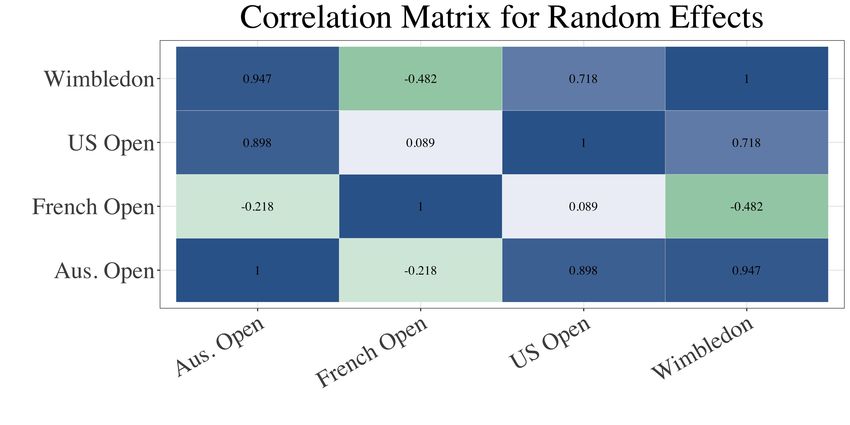
Open, and Wimbledon are all quite correlated (see Figure 12). This suggests that
after accounting for variables such as rank and opponent rank, differences in win
probability may be detectable between the French Open and the other Grand
Slams, but it is harder to detect differences among the hard courts (Australian
Open, US Open) and Wimbledon. These correlations, combined with few nonzero
random effects among top players (Figure 11), suggests that modeling ‘win’ does
not adequately capture changes in player performance at different Grand Slams.

A.1.1 Model Selection

Each of the models tested were of the form:

 ( = 1| , ) = logit−1 ( [ ] + )
 = 

 where
 {︃
 1 if match won
 =
 0 if match lost
 = IOC, Tournament, log(Rank), log(OpponentRank), age
 = Intercept, Indicator variables for tournament, year

and different combinations of and were tested. Based on AIC, the best model
excluded IOC and tournament from , and included the tournament indicators as
the only random covariates in (no random intercept). The models are summarized
in Table 11. The regression table for the fixed effects ( ) is shown in Table 10.

A.2 Modeling results of individuals

Each of the individual models for player are of the form

 ( = 1| , ) = logit−1 
 (︀ )︀

Opening up the court 17

where

 is a 1/0 variable where 1 indicates winning a point.
 is the vector of coefficients for player 
 is the matrix of data/covariates for player 
 is the number of points in the match.

We estimate ̂︀ by first selecting which covariates are important and then by
estimating the value of the coefficients for those selected covariates. Ideally, the
covariate/model selection would be performed and the coefficient value estimation
on an independent testing set. Since there were not many observations for each
player (with respect to the number of potential covariates), our model is fit on the
entire set of data.
 Model selection is done by using forward-backwards stepwise generalized linear
regression with a logit link function and by weighting the samples by the number
of total points. A minimal and maximal set of covariates is pre-determined. The
minimal set of covariates include opponent rank while the maximal set of covariates
includes opponent rank, average serve speed, % of net points won, % of aces, % of
break points won, W/UE, and their interactions with each slam. The model with
the lowest AIC is chosen, where we initialize the algorithm using the maximal set
of covariates.
 Similarly, our function model_individual() performs forward-backwards step-
wise generalized linear regression to select the best model to predict the expected
percent of points won. It first subsets the data provided to the proper individual
name and time range. Then, depending on the testing set proportion, randomly
partitions the subsetted data into a training and test set. Forwards-backwards step-
wise regression is performed on the training set and the final model and covariates
are chosen to minimize the AIC Wasserman (2004). Then the final model is then
fit to the testing set in order to obtain estimates for the coefficients. If the testing
set proportion is set to 0, the coefficient values are also estimated from the training
set and users are cautioned to be wary of using inference from these models as
model selection and model estimates are dependent on one another.

References
Andersson, H., B. Ekblom, and P. Krustrup (2008, February). Elite football on artificial turf
 versus natural grass: Movement patterns, technical standards, and player impressions.
 Journal of Sports Sciences 26, 113–22.

18 Gallagher, Frisoli, and Luby

Barnett, T. and G. Pollard (2007). How the tennis court surface affects player performance
 and injuries. Medicine and Science in Tennis 12 (1), 34–37.
Bialik, C. (2014). Wimbledon is very forgiving of players’ errors. https://fivethirtyeight.com/
 features/wimbledon-is-very-forgiving-of-players-errors/.
Gains, G. L., A. N. Swedenhjelm, J. L. Mayhew, H. M. Bird, and J. J. Houser (2010).
 Comparison of speed and agility performance of college football players on field turf
 and natural grass. The Journal of Strength & Conditioning Research 24 (10), 2613–2617.
Jurejko, J. (2018, June). French Open 2018: Why does ’King of Clay’ Rafael Nadal reign
 supreme? https://www.bbc.com/sport/tennis/44385223.
Klaassen, F. J. and J. R. Magnus (2001). Are points in tennis independent and identically
 distributed? Evidence from a dynamic binary panel data model. Journal of the American
 Statistical Association 96 (454), 500–509.
Klaassen, F. J. and J. R. Magnus (2003). Forecasting the winner of a tennis match. Euro-
 pean Journal of Operational Research 148 (2), 257 – 267. Sport and Computers.
Knottenbelt, W. J., D. Spanias, and A. M. Madurska (2012). A common-opponent stochastic
 model for predicting the outcome of professional tennis matches. Computers & Math-
 ematics with Applications 64 (12), 3820 – 3827. Theory and Practice of Stochastic
 Modeling.
Kovalchik, S. (2017). deuce: Resources for analysis of professional tennis data. R package
 version 1.0.
Kovalchik, S. A. (2016). Searching for the GOAT of tennis win prediction. Journal of
 Quantitative Analysis in Sports 12 (3), 127–138.
Leitner, C., A. Zeileis, and K. Hornik (2009). Is Federer Stronger in a Tournament Without
 Nadal? An Evaluation of Odds and Seedings for Wimbledon 2009. Austrian Journal of
 Statistics 38 (4), 277–286.
Lewit, C. (2018, September). Secrets of Spanish tennis: paradigms and superstructure.
 https://www.tennisplayer.net/public/classiclessons/chris_lewit/secrets_of_spanish_
 tennis_culture/?format=print.
McHale, I. and A. Morton (2011). A Bradley-Terry type model for forecasting tennis match
 results. International Journal of Forecasting 27 (2), 619 – 630.
Morris, B. (2013, August). Home court advantage in tennis. https://www.sbnation.com/
 tennis/2013/8/9/4599096/tennis-home-court-advantage-us-open.
Morris, B. (2015, August). Serena Williams and the difference between all-time great and
 greatest of all time. https://fivethirtyeight.com/features/serena-williams-and-the-
 difference-between-all-time-great-and-greatest-of-all-time/.
Newton, P. K. and K. Aslam (2009). Monte Carlo tennis: a stochastic Markov chain model.
Newton, P. K. and J. B. Keller (2005). Probability of Winning at Tennis I. Theory and Data.
 Studies in Applied Mathematics 114 (3), 241–269.
Paxinos, S. (2007, November). Australian Open court surface is speeding up. https:
 //www.theage.com.au/sport/tennis/australian-open-court-surface-is-speeding-up-
 20071120-ge6chj.html. The Age.
Perrotta, T. and C. Bialik (2013). It’s Very Hard to Make a Mistake at Wimbledon.
Sackmann, J. (2020, September). The Tennis Abstract Match Charting Project. https:
 //github.com/JeffSackmann/tennis_MatchChartingProject.
Sackmann, J. (2021, March). Grand Slam Point-by-Point Data, 2011-20. https://github.
 com/JeffSackmann/tennis_slam_pointbypoint.
Sipko, M. (2015, June). Machine learning for the prediction of professional tennis matches.

Opening up the court 19

Thomas, A. C., S. L. Ventura, S. T. Jensen, and S. Ma (2013). Competing process hazard
 function models for player ratings in ice hockey. The Annals of Applied Statistics 7 (3),
 1497–1524.
USTA (2018, August). 2018 US Open Wild Card Challenge. https://www.usta.com/en/
 home/pro/pro-tennis-events/us-open-wild-card-challenge.html.
Wasserman, L. (2004). All of Statistics: A Concise Course in Statistical Inference. Springer.
Wei, X., P. Lucey, S. Morgan, and S. Sridharan (2013, January). “Sweet-spot”: Using
 spatiotemporal data to discover and predict shots in tennis. In MIT Sloan Sports
 Analytics Conference Proceedings.

20 TABLES

Tables
Tab. 1: Example of the official, complete Grand Slam data. It includes winner and loser at-
tributes, match attributes, and tournament attributes. Not all attributes are shown here. We
abbreviate Winner with “W,” Loser with “L,” Points with “Pts,” and International Olympic
Committee Country Code with “IOC.”

Winner Tournament Year W IOC W Pts W Rank L Pts L Rank

Serena Williams Australian Open 2013 USA 54 3 26 15
Roger Federer Australian Open 2013 SUI 95 2 63 46
Rafael Nadal French Open 2013 ESP 140 4 115 59
Caroline Garcia Wimbledon 2013 FRA 66 100 55 47

Tab. 2: Example of a row in the secondary, partial data set.

Winner Tournament Year ... Aces Winners UE Break Points Won

Serena Williams Australian Open 2013 ... 28 10 20 5
Novak Djokovic French Open 2013 ... 5 26 31 3

Tab. 3: # of matches played for Nadal, Federer, and Williams from 2013-2019 at each of
the Grand Slams.

 Tournament Nadal Federer S. Williams

 Australian Open 32 39 35
 French Open 43 20 30
 US Open 34 31 40
 Wimbledon 23 41 35
 Total 132 131 140

Tab. 4: Regression coefficients table for the fixed effects in the mixed effects model for net
points. (Outcome variable: net_points_won)

 Term Estimate Std Error Statistic P Value

 (Intercept) -2.849 0.047 -60.821

TABLES 21

Tab. 5: Regression coefficients table for the fixed effects in the mixed effects model for aces.
(Outcome variable: aces)

 Term Estimate Std Error Statistic P Value

 (Intercept) -4.022 0.066 -61.254

22 TABLES

Tab. 9: Covariates used in each of the four hierarchical models. (Outcome variables: win,
aces, net_points_won, unforced_errors.

 Name Description Type

 late_round Indicates Round of 16 or Later Binary
 log(rank) Rank of Player, log-scale (lower = better) Continuous
 log(opponent_rank) Rank of Opponent, log-scale Continuous
 year Year of Match (2013-2019) Factor
 ATP Indicates ATP Match Binary
 tournament AO, FO, USO, or Wimbledon Factor
 IOC Country of Origin Factor

Tab. 10: Regression coefficients table for the fixed effects in the logistic model for wins
(Outcome variable: win).

 Term Estimate Std Error Statistic P Value

 log(rank) -0.705 0.015 -47.454

FIGURE CAPTIONS 23

Figure Captions

Fig. 1. Distribution of number of points for the different Grand Slams (left) and
distribution of points per match faceted by winner and loser for the two tours
(right).

Fig. 2. The percent of matches won for the first four rounds for players of the
Grand Slam home countries. A significant home court advantage does not appear
to exist in any of the Grand Slams after we account for the number of players
from a given country (the confidence intervals for each line, which are not shown,
overlap). Please note the varying number of players and matches (n) across the
individual graphs, which contribute to result variability.

Fig. 3. Performance and ranking among Spanish players at the Grand Slam
tournaments. Within the first two rounds (R128, R64), players from Spain win
more often at the French Open than other slams, but this difference is not significant.
Exploring rank, we see that the median rank of Spanish players is higher (worse),
within these two rounds, potentially providing evidence in favor of a relationship
between performance and the French Open.

Fig. 4. We see Wimbledon matches tend to have more aces and fewer unforced errors
than the other tournaments. Ellipses shown follow a multivariate t-distribution.
Each point on the figure represents one match. UE% is calculated by summing
the unforced errors of the two opponents and dividing that by the total number of
points played. The ace% is calculated similarly but with the numerator representing
the sum of both players’ aces.

Fig. 5. Player height vs. median percentage of aces per match (total aces divided
by total serves) across both the ATP and WTA Grand Slams. We confirm the
common notion that being taller is associated with being a strong server (having
a larger percent of aces). Each dot represents one player and we compute their
median ace% across all matches and all tournaments.

24 FIGURE CAPTIONS

Fig. 6. Estimated fixed effects when modeling aces, net winners, and unforced
errors.

Fig. 7. Random effects with 95% confidence intervals for 20 players in each of
the three mixed-effects models. The average random effect for each outcome and
Grand Slam across all players is shown at the bottom of each panel.

Fig. 8. Correlation matrices for random effects in the mixed effects model for Aces
(left), Points won at net (middle), and unforced errors (right).

Fig. 9. Expected value and 95% CIs of percent of points won from the individual
models for different players across differing sets of covariates. Each prediction
(below average, average, and above average) represents a different performance
level for a player at a given match.

Fig. 10. Estimated fixed effects (left) and player-level effects for Williams, Federer
and Nadal (right) under the logistic model with 95% confidence intervals.

Fig. 11. Estimated player-level effects for top performers under the logistic model
with 95% confidence intervals.

Fig. 12. Correlation matrix for random effects for the model in Eq. 3.

FIGURES 25

Figures

Fig. 1: Distribution of number of points for the different Grand Slams (left) and distribu-
tion of points per match faceted by winner and loser for the two tours (right).

Fig. 2: The percent of matches won for the first four rounds for players of the Grand Slam
home countries. A significant home court advantage does not appear to exist in any of
the Grand Slams after we account for the number of players from a given country (the
confidence intervals for each line, which are not shown, overlap). Please note the varying
number of players and matches (n) across the individual graphs, which contribute to result
variability.

26 FIGURES

Fig. 3: Performance and ranking among Spanish players at the Grand Slam tournaments.
Within the first two rounds (R128, R64), players from Spain win more often at the French
Open than other slams, but this difference is not significant. Exploring rank, we see that
the median rank of Spanish players is higher (worse), within these two rounds, potentially
providing evidence in favor of a relationship between performance and the French Open.

Fig. 4: We see Wimbledon matches tend to have more aces and fewer unforced errors than
the other tournaments. Ellipses shown follow a multivariate t-distribution. Each point on the
figure represents one match. UE% is calculated by summing the unforced errors of the two
opponents and dividing that by the total number of points played. The ace% is calculated
similarly but with the numerator representing the sum of both players’ aces.

FIGURES 27

Fig. 5: Player height vs. median percentage of aces per match (total aces divided by total
serves) across both the ATP and WTA Grand Slams. We confirm the common notion that
being taller is associated with being a strong server (having a larger percent of aces). Each
dot represents one player and we compute their median ace% across all matches and all
tournaments.

Fig. 6: Estimated fixed effects when modeling aces, net winners, and unforced errors.

28 FIGURES

Fig. 7: Random effects with 95% confidence intervals for 20 players in each of the three
mixed-effects models. The average random effect for each outcome and Grand Slam across
all players is shown at the bottom of each panel.

Fig. 8: Correlation matrices for random effects in the mixed effects model for Aces (left),
Points won at net (middle), and unforced errors (right).

FIGURES 29

 Individual model predictions
 Opponent rank = 10; reference court = French Open
 ATP − Andy Murray ATP − David Ferrer ATP − Jo Wilfried Tsonga

 Below avg. Below avg. Below avg.

 Avg. Avg. Avg.

 Above avg. Above avg. Above avg.

 ATP − Kei Nishikori ATP − Milos Raonic ATP − Novak Djokovic

 Below avg. Below avg. Below avg.

 Avg. Avg. Avg.

 Above avg. Above avg. Above avg.

 ATP − Rafael Nadal ATP − Roger Federer ATP − Stan Wawrinka

 Below avg. Below avg. Below avg.

 Avg. Avg. Avg.

 Above avg. Above avg. Above avg.
 Level of play

 ATP − Tomas Berdych WTA − Agnieszka Radwanska WTA − Angelique Kerber

 Below avg. Below avg. Below avg.

 Avg. Avg. Avg.

 Above avg. Above avg. Above avg.

 WTA − Ekaterina Makarova WTA − Madison Keys WTA − Petra Kvitova

 Below avg. Below avg. Below avg.

 Avg. Avg. Avg.

 Above avg. Above avg. Above avg.

 WTA − Serena Williams WTA − Simona Halep WTA − Venus Williams

 Below avg. Below avg. Below avg.

 Avg. Avg. Avg.

 Above avg. Above avg. Above avg.

 0.4 0.5 0.6 0.7 0.4 0.5 0.6 0.7 0.4 0.5 0.6 0.7
 Expected % of points won

 Tournament Australian Open French Open US Open Wimbledon

Fig. 9: Expected value and 95% CIs of percent of points won from the individual models for
different players across differing sets of covariates. Each prediction (below average, average,
and above average) represents a different performance level for a player at a given match.

30 FIGURES

Fig. 10: Estimated fixed effects (left) and player-level effects for Williams, Federer and
Nadal (right) under the logistic model with 95% confidence intervals.

Fig. 11: Estimated player-level effects for top performers under the logistic model with
95% confidence intervals.

FIGURES 31

Fig. 12: Correlation matrix for random effects for the model in Eq. 3.