Voxel datacubes for 3D visualization in Blender
←
→
Page content transcription
If your browser does not render page correctly, please read the page content below
Voxel datacubes for 3D visualization in Blender
                                                                                                  Matı́as Gárate1,2
                                                           1
                                                               Instituto de Astrofı́sica, Pontificia Universidad Católica de Chile, 7820436 Santiago, Chile
                                                                2
                                                                  Millennium Nucleus “Protoplanetary Disks in ALMA Early Science”, Santiago, Chile
                                                                                               Email: migarate@uc.cl
                                                                        Accepted in the Publications of the Astronomical Society of the Pacific
arXiv:1611.06965v1 [astro-ph.IM] 21 Nov 2016

                                               Abstract
                                               The growth of computational astrophysics and complexity of multidimensional datasets evidences the
                                               need for new versatile visualization tools for both analysis and presentation of the data. In this work
                                               we show how to use the open source software Blender as a 3D visualization tool to study and visualize
                                               numerical simulation results, focusing on astrophysical hydrodynamic experiments. With a datacube as
                                               input, the software can generate a volume rendering of the 3D data, show the evolution of a simulation in
                                               time, and do a fly-around camera animation to highlight the points of interest. We explain the process to
                                               import simulation outputs into Blender using the Voxel Data format, and how to set up a visualization
                                               scene in the software interface. This method allows scientists to perform a complementary visual analy-
                                               sis of their data, and display their results in an appealing way, both for outreach and science presentations.

                                               Keywords: methods: miscellaneous – methods: numerical

                                               1      Introduction
                                               The amount of data available in astronomy grows continuously in size and complexity. This creates the
                                               need to develop more effective visualizations techniques to analyze and present the data.
                                                   Typically, astronomers work analyzing datacubes, which are simply multidimensional arrays of values,
                                               such as the physical fields of hydrodynamic simulations or integral field spectroscopy data. It is easy to
                                               display the complete information of 1D arrays or 2D matrices using lineplots and colormaps. However, a
                                               problem appears for 3D datacubes, when only a single projection or a sequence of layers are displayed to
                                               visualize the dataset. This procedure comes with a reduction of the dimensionality of the data, and can
                                               cause to miss part of the information in the visual analysis.
                                                   3D visualization and Volume Rendering are now alternatives for astronomers to display 3-dimensional
                                               data (Barnes & Fluke, 2008). Current softwares and libraries allow the user to do it in real time with
                                               different levels of interactivity. Viewers like FRELLED1 (Taylor, 2015) allow to load FITS datacubes and
                                               manipulate them interactively through rotations, scaling, and mask selection. Alternatives like Virtual
                                               Reality immersions go one step forward, and let the user get inside the data to observe its features
                                               (Ferrand et al., 2016). Using these novel techniques not only allow to produce an attractive outreach
                                               material, but also provide an additional perspective of the complete dataset while doing scientific analysis
                                               along with the traditional methods(Goodman, 2012).
                                                   In this work we provide a procedure to generate a Volume Rendering from astronomical data (from
                                               numerical simulations, in particular) in the 3D graphics software Blender2 , that can be used to perform
                                               a qualitative visual analysis, and to create presentation material. Blender is free and open source, and
                                               in the recent years has shown potential as an astronomy visualization tool. Kent (2013) presents a
                                                   1 www.rhysy.net/frelled-archive.html
                                                   2 www.blender.org

                                                                                                            1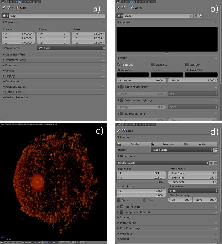
series of tutorials3 showing the software features and possible applications like: loading as halo points
a galaxy catalog or a particle simulation, use the mesh modeling tools to recreate an asteroid, and also
a demonstration of volume rendering using an image sequence. The library AstroBlend4 , developed by
Naiman (2016), provides further tools to import and display different types of astronomical data in the
interactive 3D environment of Blender, such as 3D contours and also particle simulations using halos with
a colorscale.
    A datacube can be imported into Blender through the Voxel Data format, which is the file used to
generate volumetric renderings. By importing a simulation, for example, the software can display in a
3D space one of the physical properties of interest (density, temperature, etc) using a colorscale, and
show its evolution in time. Using the Blender functions it is possible adjust the colorscale interactively to
highlight different features, incorporate a fly-around camera animation to zoom in through the relevant
regions of the datacube, and finally produce an animation to use as outreach material.
    The use of Volume Rendering provides a smooth and continuous display of the whole dataset, in
contrast with visualizations using particles or contours. Since Blender colorscale also provides control
over the transparency, it is also possible to explore the different depths of the volume without reloading
additional data.
    This article is meant to serve as a guideline for the user to convert its own data into the Voxel Data
format, learn the steps to set up a Blender scene, and render an image or a movie. Section 2 explains
the format of the voxel data files that can be used as an input to Blender. Section 3 provides simple
algorithms to convert some common simulation data formats into voxel data. In section 4 it is described
the setup process in Blender from the initial scene, through loading the Voxel Data, and finally the
rendering process. Section 5 displays examples using Gadget2(Springel, 2005) and FARGO3D(Benı́tez-
Llambay & Masset, 2016) simulations rendered in Blender.
    To complement this article, the reader can watch the tutorial series: “Blender & Astronomy Tutorial.
Using Voxel Data for 3D visualization”5 , which covers the whole process described above with real time
demonstrations in Blender. Through the article these videos will be referred as TUT:#. All the material
used for this work is available in the github repository: “Blender Bvoxer”6 , which includes the Blender
scenes, scripts to generate voxel data files, and simulation data provided by J. Cuadra and S. Perez to
test this visualization techniche. Through the article these codes will be referred as GIT:FolderName.

2        Understanding Voxel Data in Blender
This section will explain the key concepts related to the Voxel Data, which is the link between the
astrophysical data, and the 3D visualization in the Blender scene. The Voxel Data is a binary datacube
file that will serve as input for the visualization. Although the Voxel Data can be generated from a
sequence of images (as we will discuss later in this section), we prefer (and recommend) to use a single
binary file to store the information. This approach allows to represent the datacube as a single array
(which is convenient when performing operations over the data), it easier and faster to write a single
binary file than multiple images, and finally, it allows to store all the information in a compact format,
rather than in a directory. To complement this section the reader can refer to the tutorial series TUT:1
and github repository GIT:Example, where there are demonstrations for generating a simple Voxel Data
file from a function f (x, y, z).
     To visualize 3-dimensional data it is necessary to define a finite volume within the Blender scene,
this is done by creating a Cube object that will be the domain for the visualization. Once the Voxel
Data file is assigned to this domain, the 3D information stored in the file will be rendered in the Blender
scene within the boundaries of the Cube. Further technical details of the setup, such as the material and
texture settings, will be addressed later in section 4.
     The voxel file represents a datacube subdivided in the three cartesian axes (x, y, z). For each discrete
cartesian coordinate (i, j, k) inside the volume there is one voxel value V (i, j, k). Additionally, it is
possible to include multiple snapshots (frames) in the same file. This allows to show the evolution of the
datacube in time. Therefore, the Voxel Data is defined by:
    3 www.cv.nrao.edu/∼bkent/blender/
    4 www.astroblend.com/
    5 www.youtube.com/watch?v=zmY     mn6Ue2g&list=PLjFmkbKBKd0WuhhbR2MGPXZyWW7TPcNSw
    6   github.com/matgarate/Blender Bvoxer

                                                     2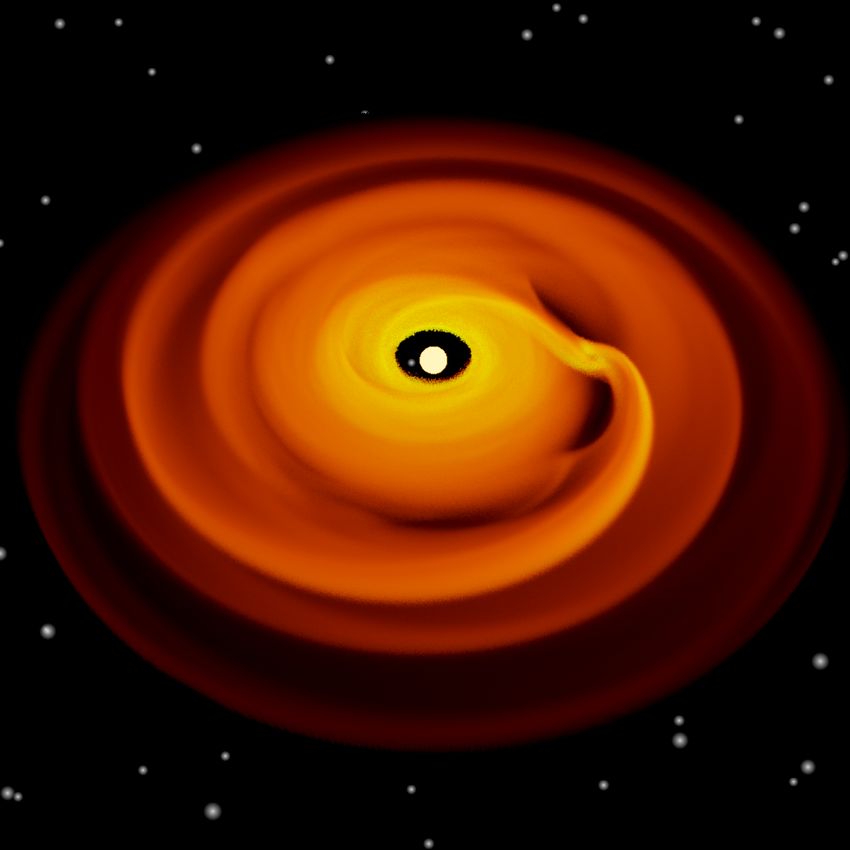
• The resolution numbers (nx , ny , nz ), that indicate the number of subdivisions of the domain in each
     axis.
   • The frame number nf , that indicates the total number of frames contained in the file.
   • (nx × ny × nz ) × nf values, which describe the astrophysical data that will be visualized inside the
     domain.

By the time of writing this article, Blender can receive the Voxel Data as an input in three different
file formats: Blender Voxel, 8bit Raw and Image Sequence. The following subsections will describe each
format, and point their advantages(+) and disadvantages(–).
     The guidelines and notation provided in this article to write both Blender Voxel and 8bit Raw file
formats are based on the description and examples available at Pythology Blogspot7 . Also, Kent (2013)
(section 4.1) provides a brief description about how to use the Image Sequence format and a complete
example on his website8 .

2.1    Blender Voxel format
The Blender Voxel format consists in a binary file that has 4 × 32bit integers in the header, corresponding
to (nx , ny , nz , nf ), followed by the (nx × ny × nz × nf ) × 32bit floating point values that represent the
actual data. For this format the values must be normalized to a [0,1] interval. The order to write the full
datacube after the header is:
  1. Frame by frame, where each frame has nz layers.

  2. Layer by layer, where each layer has ny lines.
  3. Line by line, where each line has nx values.
  4. Value by value, until completing the nx values.

The following example pseudo-code illustrates the order in which the file is written:
write([nx,ny,nz,nf])
for t from 0 to nf:
 for k from 0 to nz:
  for j from 0 to ny:
   for i from 0 to nx:
    write(Data[i,j,k,t])

   • (+) Allows high dynamic range for the data values by using 32bit floats.
   • (+) Includes a header. It only requires to input the file into Blender.
   • (+) Allows multiple frames.
   • (–) High memory usage because of using 32bit float.

We want to remark that the high memory usage may be specially troublesome when multiple frames are
stored in the Voxel Data file, since it is not possible create arbitrarily large files. For large number of
frames it may be more convenient to store each frame in a separate Voxel file, and then use the python
API of Blender to switch between frames. This will be discussed again in section 4.3.
  7 pythology.blogspot.cl/2014/08/you-can-do-cool-stuff-with-manual.html
  8 www.cv.nrao.edu/∼bkent/blender/tutorials.html

                                                          3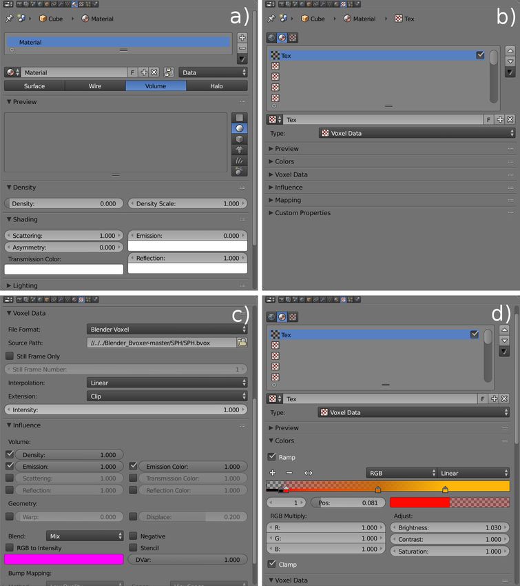
2.2    8bit Raw format
This format is a binary file of (nx × ny × nz × nf ) × 8bit integer values. The values for this format should
normalized to a [0,255] interval. The order to write the file is the same as the used for the Blender Voxel
format, the only difference is the absence of the header and the size of the values. For this format the
(nx , ny , nz ) values must be written as an input in the Blender interface. The value of nf is calculated
internally by Blender based on the file size and the previous three values.
    • (–) Low dynamic range for the data values.
    • (–) Does not include a header. It is necessary to input the resolution manually in Blender.
    • (+) Allows multiple frames.

    • (+) Memory efficient because of using 8bit integers.

2.3    Image Sequence
The Image Sequence format allows to construct a datacube using multiple images as layers. The format
consists in a directory that contains nz image files (png, for example) of nx × ny pixels. If the user
already has the tools to save his data as a set of images, this would be the most straightforward method
to construct the Voxel Data.
    The total number of images must be specified in the interface along with the image #1. The (nx ,
ny ) values are obtained from the files. Those files must be numerated to guarantee that the datacube
will be build in the correct order. For example, if there are 100 images a valid numeration would be:
name001.png,..., name100.png.
    • (+) Convenient if the images can be easily generated in order to build the datacube. This would
      save extra coding.
    • (+) Does not need a header. Blender computes the resolution automatically from the number of
      images and their dimensions.
    • (–) Only support a single frame.
    • (–) Requires multiple files.
The memory usage of this method will depend on the image number of channels and their dynamic
range. However, notice that Blender will interpret all images as monochromatic, so using anything but
a grayscale is unnecessary. The dynamic range of the grayscale will determine the level of detail. For
example, an 8bit image will provide greater detail than a 1bit image at the cost of memory usage. We
have tested this method with 1bit, 8bit grayscale images, and also with 24bit (RGB) and 32bit (RGBA)
images. Further information can be found in Kent (2013).

3     Create Voxel Data from simulation outputs
As mentioned in the previous section, the Blender Voxel and 8bit Raw inputs take the form of datacubes.
By the time of writing this article, Blender can only subdivide the visualization domain in the cartesian
axes (x, y, z). Therefore, the algorithm to construct the voxel file needs to fill each grid cell of this
datacube from the simulation data.
     For a simulation that uses an evenly spaced cartesian grid, writing the voxel data is quite straightfor-
ward, as the only thing required to do is to match (nx , ny , nz ) with the resolution of the simulation, and
scale the data values to the appropriate range before writing the file in the Blender Voxel or 8bit Raw
format. However, if the simulation is done using a cylindrical or spherical grid, a logarithmic scale, or
if it is a particle simulation (like N-Body or SPH), it is necessary to transform the space of the original
data into a cartesian datacube.
     In this section we propose methods to generate a cartesian datacube from a grid simulation in spher-
ical coordinates, and also from a particle simulation. As it is impossible to address all the possible data

                                                     4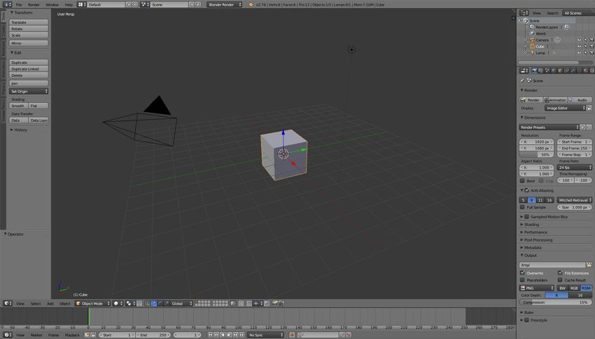
formats and methods we expect that these two should serve as good examples that the user can adjust
to his/her own needs.
    The tutorial video TUT:3 (and the second half of TUT:4) also explain these methods by going through
the example scripts, however these videos are aimed to people with little or none programming skills.
An experienced programmer will find more convenient to read the following subsections and look the
referenced codes straight away.

3.1    Spherical grid-based simulation
Converting an spherical grid into a cartesian datacube requires to fill each voxel (i, j, k) (where i ∈
[0, nx − 1], j ∈ [0, ny − 1], k ∈ [0, nz − 1]) using the spherical coordinates (r, φ, θ), which are the radial,
azimuthal and co-latitude directions in the simulation, and the physical properties F of each grid cell,
such as density, energy, temperature, etc. Notice that the spherical coordinates should indicate the middle
of the grid cell, and not the borders.
    We propose the following algorithm to perform the transformation:

  1. First transform the (r, φ, θ) coordinates into their cartesian equivalent (x, y, z).
  2. Define the cartesian boundaries of the datacube using the minimum and maximum (x, y, z) values
     from the previous step.

  3. Define a resolution (nx , ny , nz ) for the voxel datacube.
  4. For each voxel position (i, j, k) obtain its cartesian equivalent (xi , yj , zk ), using the following trans-
     formation i → xi = xmin + i · (xmax − xmin )/(nx − 1). Repeat this for j → yj and k → zk .
  5. Check if the values (xi , yj , zk ) are within the spherical boundaries of the simulation. If they do,
     proceed to the next step. If they do not, assign the voxel V (i, j, k) = 0.0. This is expected to
     happen since a spherical grid cannot fill completely the borders of a cartesian grid, or the regions
     inside the inner radial boundary of the simulation.
  6. The value of each voxel V (i, j, k) in the datacube with position (xi , yj , zk ) will be defined by the N
     closest grid cells of the simulation and their physical properties F (Ca ), with Ca the ath closest cell
     neighbor. We present two alternatives for determining V (i, j, k).

      6.1. For N = 1 use the closest neighbor as the only contribution to the voxel value. Then,
           V (i, j, k) = F (C1 ).
      6.2. For N = 8 it is possible to use a trilinear interpolation if the 8 positions (x, y, z) of the
           neighbors form a box that contains the (xi , yj , zk ) coordinate of the voxel. Then,
                                                             N
                                                             X =8
                                             V (i, j, k) =          w(Ca ) · F (Ca ),                         (1)
                                                             a=0

           where w(Ca ) is the weight for the trilinear interpolation of the grid cell Ca . (This is the
           method used in the example shown in Figure 4).
  7. After having all the voxel values, rescale them to be in the interval [0, 1] or [0, 255], depending if
     the voxel format is Blender Voxel or 8bit Raw, respectively. Notice that in the step 5 a value of 0.0
     was assigned to the voxels outside the simulation boundaries, so it may be necessary to force them
     again back to 0.0 for the visualization if the property F allowed negative values.

An implementation of this algorithm is available in the github repository GIT:Fargo3DVoxelizer, where
FARGO3D outputs are converted from an spherical grid to Blender Voxel format. Both alternatives for
steps 6.1 and 6.2 are available in the repository. While the former is enough for the visualization, it may
cause discontinuities in the sampling. On the other hand, the latter solves this problem and samples the
cartesian datacube smoothly.

                                                        5
3.2 Particle-based simulation
The process to generate a datacube from a particle simulation can be divided in two steps: First, to
define a cartesian grid and find the position of the particles on it, and second, to use the particles in each
grid cell to compute its voxel value V (i, j, k).
For a simulation with N particles, we have their position, velocities and physical properties F . The
latter can be masses and sizes for N-Body simulations, or density, thermal energy and other fluid properties
for hydrodynamic simulations like SPH (Monaghan, 1992).
We propose the following algorithm to convert an array of particles into an evenly spaced datacube:
1. Define the boundaries of the simulation using the minimum and maximum values of the particles
positions in each axis (x, y, z).
2. Define a resolution (nx , ny , nz ) that is convenient for the particle count and available memory.
3. Transform the x positions of the particles from the range [xmin , xmax ] to the range [0, nx] using
x−xmin
the linear transformation x → xv = xmax −xmin nx . Repeat for the y and z coordinates.
4. Identify if a particle P is inside (or should influence) a certain grid cell (i, j, k), and its contribution
to the voxel value V (i, j, k). For this step, we propose the following alternatives:
4.1. Simple average estimation. Truncate the transformed positions to their integer forms. A
particle P is inside a certain grid cell if the coordinates (int(xv ), int(yv ), int(zv )) match the
(i, j, k) indexes of the cell in the datacube. The value of each voxel will be given by
Nijk
X 1
V (i, j, k) = · F (Pa ), (2)
a=0
Nijk
where Pa are the Nijk particles inside a grid cell (i, j, k), and F (Pa ) is the physical property
chosen for visualization of the Pa particle. (This is the method used in the example shown in
Figure 5).
4.2. SPH interpolation. Using the interpolation method implemented in SPLASH9 (Price (2007),
section 4.1 and 4.2), the value of each voxel is given by:
N
X ma
V (i, j, k) = · F (Pa )W (r, h), (3)
a=0
ρa
where W is the SPH kernel function, r is the distance between the particle Pa and the center of
the grid cell (i, j, k), ma and ρa are the mass and density of the particle, and h = max(ha , ∆/2)
is the maximum between the smoothing length of the particle and the half width of the grid
cell.
4.3. Other possible methods could include using the N-nearest particles to influence a grid cell, and
use a customized weight functions instead the SPH kernel, such as power laws of the distance.
The value of the voxel can be computed in an analogous way as in the previous methods.
These procedures can be optimized by iterating over the particles, and adding their contribution to
the voxels that are within their range of influence, rather iterating over all the voxels and looking
for the contribution of all the N particles (Price, 2007).
5. The last step is to rescale the whole voxel datacube to have values in the interval [0, 1] or [0, 255],
depending if the voxel format is Blender Voxel or 8bit Raw, respectively.
An implementation of this algorithm is available in the github repository GIT:SPH. The example code
reads a particle list, and generates a Blender Voxel file using the density field of the particles. The
approach of step 4.1 is used for simplicity, but the interpolation recipe described by Price (2007) should
be implemented for a more accurate result, specially if the size of the grid cells is smaller than the relevant
smoothing lengths of the simulation.
9 users.monash.edu.au/∼dprice/splash/
6Figure 1: This is the default Blender scene, which includes a default Cube, a Camera and a Lamp.
With the Cube selected, it is possible to access to the Material and Texture properties in the right
panel of the interface.
4 Blender set-up for visualization
In order to produce a Volume Rendering, the light needs to pass through the defined volume, be absorbed,
scattered, and transmitted by interacting with the voxels according to their properties (density, emission,
etc), until it reaches the camera. The concept is similar to the radiative transfer process in astrophysics,
although interactions are computed in the color space, rather than in wavelenght.
This section will cover the overall steps required to load a Voxel Data file into Blender, set up
the material, render an image, and also create a fly-around camera animation. This procedure is also
demonstrated in our tutorial series TUT:2 in real time. Kent (2013) also covered the setup of a Blender
scene, going through the steps of a standard workflow.
Before starting, it is advised to take a look at the basic Blender commands, just to be able to navigate
quickly through the interface. Some pages that cover the basics are: Blender 3D Design Course - Lesson
110 by Neal Hirsig, and also the Blender Basics course11 from CG Cookie. To learn about any specific
feature of the software the reader can refer to the online Manual12 .
After opening Blender, the default scene will be displayed as shown in Figure 1.
4.1 Setup the 3D texture
Here are listed the steps to set the 3D material, starting from the default scene. The default Cube object
will act as domain for the Voxel Data as mentioned in section 2. For the complete procedure we will use
the default internal engine Blender Render, which allows to use customized voxel files as input.
1. Right-clicking on the default Cube gives access to the object properties, including the Material
and Texture properties. Select the Material property, set the type to Volume and Density =
0.0 (see Figure 2 (a)). The integration of the light rays through the volume can be customized
in the Integration panel through the Step Size and the Depth Cutoff, both parameters can
be adjusted to improve the accuracy at the cost of rendering time. More details about the other
Volume Rendering settings can be found in its respective section in the manual13 .
10 gryllus.net/Blender/Lessons/Lesson01.html
11 cgcookie.com/course/blender-basics/
12 www.blender.org/manual/
13 www.blender.org/manual/render/blender render/materials/special effects/volume.html
72. Select the Texture property and set the type to Voxel Data (see Figure 2 (b)). In the Voxel
Data panel select the file format to one of the discussed in the section 2 (see Figure 2 (c)). If
the datacube used contains only a single frame (nf = 1), then check the Still Frame Only, and
set the Still Frame Number = 1 to display the frame. For nf > 1 leave Still Frame Only
unchecked. In this case the Current Frame value of the Blender Timeline will determine which
frame of the datacube should be displayed.
3. In the Influence panel check the Density, Emission and Emission Color fields, and set them
all to 1.0 (see Figure 2 (c)). The Influence panel determines which parameters of the volume
will be defined from the Voxel Data input. The Density field defines the opacity of the volume,
the Emission defines its brightness, and Emission Color allows to use a colorscale that can be
customized in the Color panel, instead of a grayscale.
4. In the Color panel check the Ramp option (see Figure 2 (d)). The ramp is a function that receives
the values of the Voxel Data file as a position between 0.0 and 1.0, and returns the color specified
at that position (notice that it is also possible to control the transparency with the α channel,
allowing see through or completely hide a range of values). Selecting the sliders allows to control
their position in the ramp, and the color output. For the interpolation we suggest to start using
the RGB color mode, and select the Linear method for the transition between consecutive sliders.
The reader is encouraged to experiment with the other non-linear interpolation methods available
in order to find the colorscale that best suits the data. Finally, adjusting the Brightness and
Contrast helps to highlight the features of the volume and to expose its internal structure. This
last part is mostly a process of trial and error, and may depend on the resolution of the Voxel
Data file.
4.2 World, Camera and Render
The following steps consist in the scene adjustments, positioning of the camera, correct the cube scaling,
and other tweaks to improve the quality of the visualization.
1. Start by deleting the default Lamp object, since the datacube will illuminate by itself.
2. It is recommended to scale up the Cube object in order to resolve better the volume (see Figure 3
(a)). It is advised to use a scale consistent with the geometry of the simulation, for example, the
scale of a disk simulation in the z axis should be smaller than the scale of the x and y axes.
3. In the World properties it is convenient to set the Horizon color to black in order to increase the
contrast between the Voxel Data and the background (see Figure 3 (b)).
4. To have a preliminary visualization of the Voxel Data switch the Viewport Shading to Rendered.
The viewport should look like Figure 3 (c). This mode can be used to explore the data interactively,
and to adjust the color, brightness and contrast in the Texture property in real time.
5. To render a quick image, orient the Camera looking toward the Cube object, and position it at a
distance such that the volume is contained inside the Camera field of view. There are many ways
to do this and can be learned from every basic tutorial, but for now it is advised to use the command
Align Camera to View. Then, select the resolution of the image in the Render properties and
press Render (see Figure 3 (d)).
6. If the datacube contains multiple frames to generate an animation (nf > 1), select the Start Frame
and End Frame to go from 1 to nf , remember to leave unchecked the Still Frame Only option
in the Texture properties. Then, go to the Output panel in the Render properties, choose a
destination and format for the movie file, and press the Animation button.
8Figure 2: Steps to import the Voxel Data and set up the 3D texture. (a) Set the Material to Volume
and Density to 0.0. (b) Set the Texture Type to Voxel Data. (c) In the Voxel Data panel, set file
format to Blender Voxel or 8bit Raw (this last one requires to specify the dimensions of the datacube),
and load the datacube file. In the Influence panel, set the Density, Emission, and Emission Color
to 1.0. (d) In the Color panel, activate the Color Ramp, then adjust the sliders to customize your
colorscale, adjusting the Brightness and Contrast may help to highlight the features of the datacube.
4.3 Other setup tools
Different setup tools can help to produce more appealing results. Here, we listed some of them, but since
illustrating each step would greatly extend the length of this section, these will only be explained briefly.
These are standard methods in Blender that can be found in many video tutorials, including tutorials
TUT:2 and TUT:4.
• Camera Fly-Around: The Camera can be constrained to move in time through a customized path,
and kept pointing toward the object of interest. This allows to focus on the different regions of
the simulation as it evolves in time, or simply go around all the details of a single frame of the
datacube.
The overall procedure is:
– Create a Bezier Curve or Bezier Circle, and go to Edit Mode in order to customize the
animation path.
9Figure 3: Steps to generate a quick render. (a) Rescale the Cube object in the Object properties.
(b) In World properties, set the Horizon color to black. (c) In the 3D viewport, set the Viewport
Shading to Rendered in order to previsualize the datacube. (d) In the Render properties select the
image dimensions. Press Render to generate a single image, or Animation to render a movie in the
defined Output location.
– In the Curve properties check the Path Animation and set the number of frames needed to
go through the whole path.
– To animate the Evaluation Time set it to 0.0 at the starting frame, right click of the value
slider and select Insert Keyframe. Repeat this last step at the final frame with a different
value for the Evaluation Time. This will cause the Evaluation Time to change between
the selected values during the animation.
– Reset all the position and rotation values of the Camera object to 0.0.
– Then, in the Constraints properties add the Follow Path constraint. Set the Bezier Curve
as the Target object, the Y axis to point forward, the Z axis to point upwards.
– Add the Track To constraint, and set the Cube as the target object, the -Z axis to point
towards the Cube, and the Y axis to point upwards.
– By pressing Play you should see the camera following the specified path.
– An optional method is to create an Empty Object, and use it as the focus of the Camera
in the Track To constraint. Animating the position of this object allows to move the camera
focus point through the animation.
10• Adding Halo-Points: As the data is related to astronomical subjects, it may be appealing to include
a nice background if the audience is non-scientific. The Halo Points are ideal to simulate stars in
the background of the scene.
– Add any Mesh object and switch from Object Mode to Edit Mode.
– Select all the vertices and use the Merge at Center command to collapse them into a single
vertex.
– In the Material property, switch the type to Halo. Use Size and Hardness values to control
the appearance of the halo.
– To add multiple halo points at once, create an object like a Sphere, and in Edit Mode use
the command Delete Edges and Faces. Repeat the material setup to produce as many halo
points as vertices had the object.
• Compositor Post-Processing: The previous sections showed how to set up a Color Ramp for the
datacube. However, while the Brightness and Contrast values help to highlight the features of
the data, these do not always produce a colorscale that favors the image as a whole. By switching
from the 3D View to the Node Editor it is possible to post-process the rendered image for more
appealing results. One useful node is the Color Balance, which corrects the image Shadows,
Midtones and Highlights through the Lift, Gamma and Gain colors respectively.
• Switch Voxel Data files with python: It is also possible to automatize some of the tasks done in the
interface using the Blender API for python scripting. As was noted in section 2, storing a whole
simulation in a single Voxel Data file can be inconvenient for long (or even moderate) simulations.
In this case, it is easier to have one voxel file for each snapshot and perform the switch every frame
through a script.
In the python script import the bpy library (Blender internal library), and iterate over the frame
count. Then, in each frame assign the corresponding voxel file to the texture, render the image, and
save it. The individual images can be joined in a single video with the Blender Movie Editor, or
with an external program. An example script for this process is available in the github repository
GIT:VoxelAnimation.
5 Examples
The Voxel Data visualization described in this work was tested for Gadget2 and FARGO3D simulation
outputs. The Gadget2 code uses the lagrangian formalism with the Smoothed Particle Hydrodynamics
(SPH) method, while FARGO3D uses the eulerian formalism and support cartesian, cylindrical, and
spherical grids.
The image shown in Figure 4 was rendered using FARGO3D outputs provided by S. Perez. The figure
shows a protoplanetary disk with a giant planet embedded, and the between the planet and the gas. The
planet gravity opens a gap along its orbit and excites the spiral wakes that propagate through the disk.
Central and surrounding stars were included for aesthetic reasons. The available video animation14 shows
the gap opening process and the circumplanetary disk that surrounds the planet.
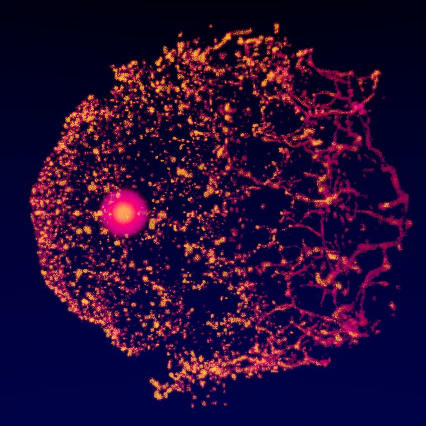
The image shown in Figure 5 was rendered using Gadget2 outputs provided by J. Cuadra. The
figure shows the stellar winds emitted by a Wolf-Rayet star as it moves through the galactic center, and
how the ejected material form clumps by cooling in the interstellar medium. The available turn-around
animation15 also shows that the clumps are distributed in a ‘parabolic shell’, rather than through all the
space (as could be misinterpreted by using a projection view).
In both examples (images and videos) we illustrated different animation techniques that help to
highlight the particular features of each simulation, such as the circumplanetary region or the clump
distribution. We also encourage the reader to explore more features of the software, in order to find the
most effective way to present its own work, and guide its audience through the data visualization.
14 www.youtube.com/watch?v=ahf3J 6iv3s
15 www.youtube.com/watch?v=IQh-rvOLtdQ
11Figure 4: Protoplanetary disk with a massive planet carving a gap. Simulation data provided by S.Perez
using FARGO3D, the output was converted from an spherical grid as described in the section 3.1. The
image was post-processed to brighten the colors, and the halo points were added to emulate surrounding
stars.
Figure 5: Stellar winds from a Wolf-Rayet star moving through the galactic center (Cuadra et al., 2008).
Simulation data provided by J. Cuadra. The output was converted from an SPH simulation as described
in section 3.2. The image was post-processed to brighten the colors, and also the Blend Sky option of
the World properties was used to add the background colors.
126 Summary
We have discussed how to use the Volumetric Rendering features of the software Blender to display the
results of astrophysical simulations. We have described the Voxel Data formats, which are binary files
(or image sequences) used to import a datacube into the Blender interface, and discussed the advan-
tages and disadvantages of each one in terms of flexibility and memory usage. In this context, we have
proposed algorithms to convert simulation outputs (either grid or particle based) into a voxel datacube,
and provided examples using stellar winds Gadget2 simulations, and protoplanetary disks FARGO3D
simulations.
In the Blender interface we showed the process of setting up a scene, loading the Voxel Data file, and
adjusting the colorscale to render an image. We have also presented some basic tools, such as color bal-
ance corrections and camera-fly around animation, that may help to create appealing outreach material.
The whole process is available in our mentioned Youtube tutorial series “Blender & Astronomy Tu-
torial. Using Voxel Data for 3D visualization”. We want to mention that though this article was focused
on representing numerical simulations, the overall procedure is the same if the information can be stored
in a datacube.
The use of Volume Rendering and 3D visualization offers a whole new range of possibilities to perform
complementary data analysis and to display our results for the public. Softwares like Blender present
many useful tools to accomplish this task. Furthermore, along with the evolution of computer graphics
more alternatives will be available, allowing us to create more detailed and effective visualizations.
7 Acknowledgements
We would like to thank Jorge Cuadra and Sebastián Perez for providing their simulation data to test
this visualization procedure, and Pablo Benı́tez-Llambay for his collaboration in the development of the
FARGO3D to Voxel Data converter. We thank S. Perez, P. Benı́tez-Llambay, and D. Calderón for their
comments in the early version of this paper, and also to the anonymous referee for the comments and
suggestions to improve this article. The author acknowledges financial support from the Millennium
Nucleus RC130007 (Chilean Ministry of Economy) and the associated PME project: “MAD Community
Cluster”, from FONDECYT grant 1141175, and Basal (PFB0609) grant. The Geryon clusters housed
at the Centro de Astro-Ingenieria UC were used for the SPH calculations of this paper. The BASAL
PFB-06 CATA, Anillo ACT-86, FONDEQUIP AIC-57, and QUIMAL 130008 provided funding for several
improvements to the Geryon clusters. The FARGO3D simulations used in this work were performed in
the Belka cluster, financed by FONDEQUIP project EQM140101 and housed at MAD/Cerro Calan.
References
Barnes, D. G., Fluke, C. J., 2008, New Astronomy, 13, 599
Benı́tez-Llambay, P., Masset, F.S., 2016, ApJS, 223, 11
Cuadra, J., Nayakshin, S., Martins, F., 2008, MNRAS, 383, 458
Ferrand, G., English, J., Irani, P., 2016, arXiv:1607.08874
Goodman, A. A., 2012, Astronomische Nachrichten, 333, 505
Kent, B. R., 2013, PASP, 125, 731
Monaghan, J. J., 1992, ARA&A, 30, 543
Naiman, J. P., 2016, Astronomy and Computing, 15, 50
Price, D. J., 2007, PASA, 24, 159
Springel, V., 2005, MNRAS, 364, 1105
Taylor, R., 2015, Astronomy and Computing, 13, 67
13This is an author-created, un-copyedited version of an article accepted for publication in Publications of
the Astronomical Society of the Pacific. IOP Publishing Ltd is not responsible for any errors or omissions
in this version of the manuscript or any version derived from it.
14You can also read