CONTINUOUS PRODUCTIVITY IMPROVEMENT USING IOE DATA FOR FAULT MONITORING: AN AUTOMOTIVE PARTS PRODUCTION LINE CASE STUDY - MDPI
←
→
Page content transcription
If your browser does not render page correctly, please read the page content below
sensors
Article
Continuous Productivity Improvement Using IoE Data for Fault
Monitoring: An Automotive Parts Production Line Case Study
Yuchang Won              , Seunghyeon Kim, Kyung-Joon Park                     and Yongsoon Eun *

                                           Department of Information and Communication Engineering, Daegu Gyeongbuk Institute of Science and
                                           Technology, Daegu 42988, Korea; yuchang@dgist.ac.kr (Y.W.); seu7704@dgist.ac.kr (S.K.); kjp@dgist.ac.kr (K.-J.P.)
                                           * Correspondence: yeun@dgist.ac.kr

                                           Abstract: This paper presents a case study of continuous productivity improvement of an automotive
                                           parts production line using Internet of Everything (IoE) data for fault monitoring. Continuous
                                           productivity improvement denotes an iterative process of analyzing and updating the production
                                           line configuration for productivity improvement based on measured data. Analysis for continuous
                                           improvement of a production system requires a set of data (machine uptime, downtime, cycle-time)
                                           that are not typically monitored by a conventional fault monitoring system. Although productivity
                                           improvement is a critical aspect for a manufacturing site, not many production systems are equipped
                                           with a dedicated data recording system towards continuous improvement. In this paper, we study the
                                           problem of how to derive the dataset required for continuous improvement from the measurement
                                           by a conventional fault monitoring system. In particular, we provide a case study of an automotive
                                           parts production line. Based on the data measured by the existing fault monitoring system, we model
                                           the production system and derive the dataset required for continuous improvement. Our approach
                                 provides the expected amount of improvement to operation managers in a numerical manner to help

                                           them make a decision on whether they should modify the line configuration or not.
Citation: Won, Y.; Kim, S.; Park, K.-J.;
Eun, Y. Continuous Productivity
                                           Keywords: internet of everything; production systems engineering; continuous productivity im-
Improvement Using IoE Data for
                                           provement; smart factory; fault monitoring data
Fault Monitoring: An Automotive
Parts Production Line Case Study.
Sensors 2021, 21, 7366. https://
doi.org/10.3390/s21217366
                                           1. Introduction
Academic Editor: Paolo Bellavista               Collecting operation data from production systems in the factory floor has been
                                           a critical task to maintain the system operation and productivity. Most existing data
Received: 11 October 2021                  collection systems are intended to monitor faults that are occurring from various machines
Accepted: 2 November 2021                  in the system. Some are automated to raise alarms in ab-normalcy [1], and others rely on
Published: 5 November 2021                 manual data collection and feed them to tools such as statistical process control [2]. Recently,
                                           thanks to the rapid advances of the Internet of Everything (IoE) technology, automated data
Publisher’s Note: MDPI stays neutral       collections are receiving a great deal of attention in the era of smart factory and Industry
with regard to jurisdictional claims in    4.0 with visions of using them beyond the fault detection and isolation: for preventive
published maps and institutional affil-    maintenance, job scheduling, productivity improvement, and various optimization [3,4].
iations.                                   Indeed, ref. [5] proposes to use an IoT-based architecture that collects information regarding
                                           key performance indicators to improve productivity, refs. [6–8] propose to build a digital
                                           twin for the production systems for multi-purpose optimization, ref. [9] suggests a smart
                                           factory framework, which has a cloud-assisted and self-organized structure to produce
Copyright: © 2021 by the authors.          customized products in a real-time manner, and [10] suggests an IoT-based supply chain
Licensee MDPI, Basel, Switzerland.         management system that tracks locations of goods to help managers check the status of a
This article is an open access article     supply chain and its dependencies.
distributed under the terms and                 An important issue that can be addressed using the infrastructure of IoE enabled smart
conditions of the Creative Commons         factory is the continuous improvement of a production line [11]. The continuous improve-
Attribution (CC BY) license (https://
                                           ment is a major tool for production systems management, where projects are designed to
creativecommons.org/licenses/by/
                                           improve productivity of the production systems. Specifically, continuous improvement
4.0/).

Sensors 2021, 21, 7366. https://doi.org/10.3390/s21217366                                                       https://www.mdpi.com/journal/sensors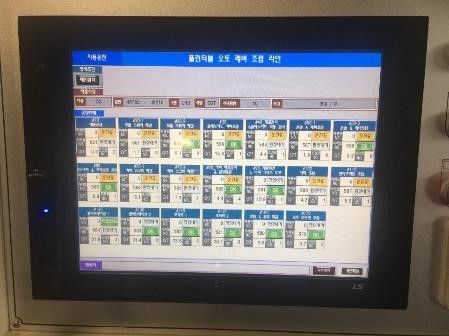
Sensors 2021, 21, 7366                                                                                            2 of 16

                         projects involve bottleneck identification and elimination by allocating additional resources
                         in order to achieve higher productivity in an efficient manner. In addition, analysis for
                         the continuous improvement requires the capability of quantifying the improvement if
                         characteristics of the bottleneck are changed. Existing studies [12] for methods of bottleneck
                         identification and analysis for continuous improvement projects are based on measurement
                         data, such as cycle-time (average time for a machine to finish a task), uptime (average
                         time for a machine to be up, i.e., operational), downtime (average time for a machine to be
                         down, i.e., not operational), and buffer capacity.
                               We point out that hardly any manufacturing facilities has dedicated IoE devices for
                         direct measurement of cycle-time, uptime, and downtime for the continuous improvement
                         while many facilities have basic fault monitoring systems. Unfortunately, cycle-time,
                         uptime, and downtime are not directly available from fault monitoring systems. For
                         example, the fault monitoring system in [13] represents machine states as ‘processing’,
                         ‘inspection’, and ‘manual operation’ and that of a microfluidic device manufacturing
                         line [14] categorizes machine states as ‘no operation’, ‘idling’, and ‘operating’. A monitoring
                         system in an automotive part production line that is used for a case study in this work
                         categorizes machine states as ‘working’, ‘idling’, ‘complete’, and ‘alarm’. Clearly, extracting
                         cycle-time, uptime, and downtime of each machine from the mentioned fault monitoring
                         data are not at all straightforward. Although many manufacturing facilities are installing
                         IoE devices for data collection under the initiative of smart factory and Industry 4.0, the new
                         devices are still installed with the main purpose of monitoring faults [15].
                               A method of using the data from the existing fault monitoring IoE systems for the
                         purpose of the continuous improvement would save time and resource for the manufactur-
                         ing facilities: new installation is not necessary which may avoid stopping the production
                         for the installation. Thus, in this paper, we present a case study where the continuous
                         improvement of an automotive parts production system is addressed using the data from a
                         fault monitoring system. As mentioned earlier, the dataset necessary for the continuous
                         improvement (i.e., uptime, downtime, and cycle-time) are not directly available from the
                         fault monitoring systems. Therefore, we study the problem of how to derive the dataset of
                         uptime, downtime, and cycle-time for the continuous improvement from the existing fault
                         monitoring data.
                               In order to model and analyze production systems, many approaches and frameworks
                         are available as reviewed in [16]. In this work, as a main tool for productivity analysis,
                         we use the theory of production systems engineering (PSE) [11] due to three distinct
                         advantages: evaluation of various performance metrics is possible for production systems;
                         convergence of the numerical algorithm in PSE is analytically proven; and it has been
                         applied to various actual manufacturing systems.
                               The theory of PSE models a production line with machines and buffers, where ma-
                         chines are characterized by uptime, downtime, and cycle-time. The aggregation algorithm
                         approximates the model of the serial production line as one virtual machine by aggregating
                         the consecutive two machines and one buffer, recursively. Using this aggregation algorithm,
                         the theory of PSE provides the foundation of modeling production systems and predicting
                         performance characteristics, such as throughput, transient [17,18], lean buffering [19], lead
                         time [20], bottleneck machine, and bottleneck buffer [12].
                               The aggregation algorithm is analytically proven to converge [11]. This is a significant
                         advantage compared to other methods. For instance, the convergence of the ADDX
                         algorithm used in the decomposition approach [21] is not analytically guaranteed.
                               Various productivity analysis cases based on the theory of PSE have been reported (an
                         automotive paint shop line [22], a lighting equipment assembly line [23], a ham shaving and
                         packaging line [24], and a gear assembly line in a motorcycle powertrain manufacturing
                         plant [25]).
                               Finally, several major manufacturing companies appear to have in-house tools and
                         methods, but these are not publicly available. Discrete event simulations could be an
Sensors 2021, 21, 7366                                                                                              3 of 16

                         alternative approach, but are computationally much heavier than the methods PSE provide,
                         especially, when number of machines and capacity of buffers are large.
                              Our case study pertains to an automotive part production line. The line has a fault
                         monitoring system that observes the status of all the machines in the production sys-
                         tem. We present a method of extracting uptime, downtime, cycle-time from the fault
                         monitoring data. Then, based on PSE, we model the production line with appropriate
                         parameters. In turn, we use this model to address continuous improvement projects under
                         various scenarios.
                              The main contributions of this paper are as follows:
                         •    We propose a concept of using existing fault monitoring data for the purpose of
                              continuous improvement of production systems;
                         •    We present a case study using an automotive parts production line;
                         •    We develop a mathematical model of the line that predicts key performance character-
                              istics, such as throughput, lead time, bottleneck machine, and bottleneck buffer;
                         •    Based on the model, we develop a continuous improvement scenario that leads to up
                              to 10% of productivity improvement.
                              The outline of the rest of the paper is as follows. Section 2 describes the production
                         line we consider. Additionally, description of the fault monitoring data are given. In
                         Section 3, we discuss the challenges why fault monitoring data are not directly transferable
                         to uptime, downtime, and cycle-time. Then, we introduce a method of conversion for this
                         particular production line considered. Based on the estimated parameters, we create a
                         model and analyze the production line with the theory of PSE in Section 4. Section 5 shows
                         the continuous improvement results in a few scenarios. Finally, conclusions are presented
                         in Section 6.

                         2. Automotive Parts Production Line and Fault Monitoring Data
                         2.1. Production Line
                                The plant covered in this paper is an automotive parts assembly line from a tier-1
                         vendor for a world top-5 motor company. We consider an automotive parts production
                         line whose simplified illustration is shown in Figure 1. The line comprises 20 assembly
                         machines connected serially. We refer to each machine by mi , i = 1, 2, · · · , 20 in the order
                         of the part flow in the production system. The machines m1 and m20 are semi-automatic,
                         i.e., operated by human workers and the rest are automatic. Machines assemble sub parts
                         and inspect defectiveness of products. Sub parts and assembled parts are moving on pallets
                         in the production line. Each pallet is identified by an RFID, the reader of which is installed
                         on all machines in the line. There are various assisting devices to some machines that
                         provide necessary materials (screw, lubricants, etc.). Semi-assembled products are placed
                         on a pallet and moved to the next machine.
                                All machines are connected by the pallet conveyor system. The pallet conveyor
                         system transfers pallets from m1 to m19 . After passing m19 , pallets return to the first
                         machine. The total number of pallets is 40. The pallet conveyor system has stoppers to
                         block the pallet from getting into the machine. The stopper is in front of the entrance of
                         the machine as shown in Figure 1. All pallets stop at the stopper once. If the machine is
                         full, a pallet waits at the stopper until the machine is empty. If not, then the pallet goes into
                         the machine.
                                Among 20 machines, m15 , m16 are identical, and m17 , m18 are also identical to each
                         other. This is because the task by m15 and m17 are taking about twice as much time as the
                         other tasks. Hence, two identical machines are allocated for the job in order to speed up
                         the process. Their operations are as follows. If m15 operate only on the parts delivered by
                         even numbered (pallet RFID) pallets. It passes the odd numbered pallets to m16 . The other
                         pair m17 and m18 are operated in a similar manner.
Sensors 2021, 21, 7366 4 of 16
Assembly Machine Automotive Parts
Monitoring System Logging System
Assistant Devices Pallet
Stopper
Wired Network Human
Worker
…
…
Figure 1. Automotive parts production line with fault monitoring and logging system.
The machines m2 , m6 , m9 operate with block before service (BBS) and the other ma-
chines operate with block after service (BAS), where BAS and BBS are rules for interacting
between machines and buffers. When the downstream buffer of a machine is full, the ma-
chine should stop producing. In this situation, the machine with the BAS rule produces
one product and keeps it inside the machine. On the other hand, the machine with the BBS
rule does not produce and leaves its inside space empty [11].
The line produces a total of 52 types of products. The machines need to change
their settings whenever the types of products change. It takes time to change the settings,
therefore the company operates the line with a batch production rule to reduce the process
change time where the batch refers to a group of products of the same type. As the
machines are differently operated by the product type, the throughput of the line may also
be different product types.
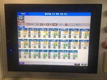
Figure 1 also shows a fault monitoring system. Every machine transfers its operation
data to the fault monitoring system at every second. The monitoring system represents
all machine’s states right after receiving the operation data from each machine. The fault
monitoring system in this manufacturing facility does not record data perhaps because it is
designed only for raising alarm at faults. We develop the logging system which takes all
data from the monitoring system and write the data to a file by the hour.
The machines rarely produce defective products. Nevertheless, the line has the
capability built in to deal with the defective parts. The defective products are not removed
from the production line immediately. If a machine generates a defective product, then the
machine informs to the monitoring system. After that, the monitoring system transmits the
serial number of the defective product to the downstream machines so that the downstream
machines just pass the defective product until m11 or m19 , which are inspection machines.
The inspection machines eliminate defective parts into their basket.
The production line operates for 24 h with several break times.
2.2. Fault Monitoring Data
Using the logging system described in the previous subsection, we obtained fault
monitoring data for five months in 2019. The fault monitoring data contain machine state,
product state, processing time, serial number, and logging time. An example of the data is
shown in Table 1, where ‘Time’, ‘Type’, ‘M State’, ‘P State’, ‘SN’, and ‘PT’ refer to ‘Logging
Time’, ‘Product Type’, ‘Machine State’, ‘Product State’, ‘Serial Number’, and ‘Processing
Time’, respectively.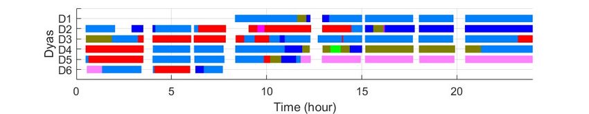
Sensors 2021, 21, 7366                                                                                                     5 of 16

                                 Table 1. Example of the operation data recorded by the logging system.

                                                m1                                         m2                      m3      ···
   Time         Type
                         M State        P State      SN       PT      M State      P State      SN        PT     M State   ···
 08:37:29         P1     Working       Stand by      123      5.7    Complete        OK         120       13.5    Idling   ···
 08:37:30         P1     Working       Stand by      123      6.7      Idling        OK         120       13.5    Idling   ···
 08:37:31         P1     Working          OK         123      7.7      Idling        OK         120       13.5   Working   ···
 08:37:32         P1     Working          OK         123      8.7      Idling        OK         120       13.5   Working   ···
 08:37:33         P1     Working          OK         123      9.7     Working     Stand by      121       0.2    Working   ···
 08:37:34         P1     Complete         OK         123      9.7     Working     Stand by      121       1.2    Working   ···
 08:37:35         P1      Idling          OK         123      9.7     Working     Stand by      121       2.2    Working   ···
 08:37:36         P1      Idling          OK         123      9.7     Working     Stand by      121       3.2    Alarm     ···
 08:37:37         P1      Idling          OK         123      9.7     Working     Stand by      121       4.2    Alarm     ···
 08:37:38         P1      Idling          OK         123      9.7     Working        OK         121       5.2    Alarm     ···
 08:37:39         P1     Working       Stand by      124      0.2     Working        OK         121       6.2    Alarm     ···
 08:37:40         P1     Working       Stand by      124      1.2     Working        OK         121       7.2    Alarm     ···
 08:37:41         P1     Working       Stand by      124      2.2     Working        OK         121       8.2    Alarm     ···
 08:37:42         P1     Working       Stand by      124      3.2     Working        OK         121       9.2    Alarm     ···
 08:37:43         P1     Working       Stand by      124      4.2    Complete        OK         121       9.2    Alarm     ···
 08:37:44         P1     Working          No         124      5.2    Complete        OK         121       9.2    Alarm     ···
 08:37:45         P1     Working          No         124      6.2    Complete        OK         121       9.2    Alarm     ···
      ..           ..       ..             ..         ..       ..         ..          ..         ..        ..       ..     ..
       .            .        .              .          .        .          .           .          .         .        .          .

                                        The item ‘Machine State’ in the operation data indicates the operate state of the
                                   machine at a specific time. The machine reports its state by ‘Idling’, ‘Working’, ‘Complete’,
                                   or ‘Alarm’. The detailed description of ‘Machine State’ are as follows:
                                   •     A machine reports ‘Idling’ when the inside of the machine is empty;
                                   •    A machine reports ‘Working’ when the machine does assembling, inspecting, or other
                                        actions for producing products;
                                   •    A machine reports ‘Complete’ after finishing production processes, and sustains
                                        ‘Complete’ until its inside becomes empty;
                                   •     A machine reports ‘Alarm’ if the machine is in a breakdown.
                                        The item ‘Product State’ represents the inspection results of the defectiveness of the
                                   assembled product. The machine informs the state of the product as ‘Stand by’, ‘OK’,
                                   and ‘NO’.
                                   •     A machine represents ‘Product State’ as ‘Stand by’ after the machine takes a product;
                                   •     After finishing the inspection, the machine reports ‘Product State’ as ‘OK’ if there is
                                         no problem with the product;
                                   •     If the machine identifies defective parts, then the machine reports ‘Product State’
                                         as ‘NO’.
                                         The rest of the data include ‘Serial Number’, ‘Processing Time’, ‘Time’, and ‘Type’.
                                   The item ‘Serial Number’ refers to the sequence of products during a day. The monitoring
                                   system initiates ‘Serial Number’ to 1 at midnight. The monitoring system sequentially
                                   assigns ‘Serial Number’ to pallets by reading RFID at the first machine, and removes it at
                                   m19 . The item ‘Processing Time’ indicates how long the pallet stays inside the machine for
                                   producing. The item ‘Time’ indicates when the log is recorded, and ‘Type’ represents a
                                   product type in the first machine.
Sensors 2021, 21, 7366 6 of 16
3. Obtaining Uptime, Downtime, Cycle-Time from the Fault Monitoring Data
Obviously, the data shown in Table 1 are not in a form from which the uptime,
downtime, and cycle-time of each machine are obtained in a straightforward manner.
As we pointed out in the introduction, this is due to that the fault monitoring data collection
are not intended for continuous productivity improvement. This difficulty of mismatch is
dealt with in detail in Section 3.2.
Additionally, as alluded to in Section 2.2, uptime, downtime, and cycle-time may be
different by the types of the product. Hence, the first step is to isolate the time segment
where a given product type is produced. Therefore, we propose a parameter estimation
method consisting of two stages, a preprocessing stage and an estimating stage. The prepro-
cessing stage is trimming the fault monitoring data: removing the break time from the log,
classifying the product types, and removing the logs that corresponds to initial transient
state. The parameters, uptime, downtime, and cycle-time, are estimated by the second
stage based on the trimmed data. The entire procedure for estimating the parameters are
simplified in Figure 2.
Operation Data Daily File Trimmed data
ZĞŵŽǀŝŶŐ
ƵƉͬĚŽǁŶƚŝŵĞĞƐƚŝŵĂƚŝŽŶ
ĂƚĞŐŽƌŝnjŝŶŐ
ĐLJĐůĞƚŝŵĞĞƐƚŝŵĂƚŝŽŶ
dƌŝŵŵŝŶŐ
Monitoring System Automated Logging System Preprocessing Stage Estimating Stage
Figure 2. Parameter estimation procedure.
3.1. Preprocessing Stage
Figure 3 shows typical daily operation of the production line for a week in the Month
4 of 2019. This snapshot of the operation data is obtained as follows. First, break time had
to be determined from the logs. For this purpose, we use the ‘SN’ of m1 : if ‘SN’ of m1 does
not change for more than 10 min, we determine that the production line is not operational
(break time for the workers). The color of the bar represents different product types. This is
determined by the ‘Type’ data in m1 from the fault monitoring dataset. We point out that
Figure 3 is the result of preprocessing that identifies in automatic manner the break time
and the types.
P1 P2 P3 P4 P5 P6 P7
Figure 3. Daily operations (determined by the idle time of m1 ). Different part types are shown by different colors. Data
from Month 4 in 2019. The line produces multiple types of parts in a day. Most breaks are planned, but others exist due to
unexpected (either workers or machines) situations.Sensors 2021, 21, 7366 7 of 16
From Figure 3, one may use all the data segment with the same color to extract the
cycle-time of each machine. However, for uptime, another aspect must be taken into
account. When the machine is in transient state, total operation time may not be accurate,
which affects the calculation of uptime (uptime is computed by subtracting downtime from
the total operation time). Hence, we additionally remove the first portion of the data until
the last machine completes five products. Therefore, we cut the data related to the first
five products off in the fault monitoring data in order to generate trimmed data.
3.2. Estimating Stage
The purpose of this stage is to extract uptime, downtime, and cycle-time of individual
machine (from m1 tot m20 ) for a given product type. Trimmed segments for a given product
(same color in Figure 3) are used.
We first discuss how to obtain a cycle-time for each machine. The cycle-time is
identified by searching ‘Idle’-‘Working’-‘Complete’ states sequence in the fault log. This is
illustrated in Figure 4. It may appear that after find the sequence, use ‘Working’ state as
one instantiation of the cycle-time may suffice. However, after observing the operation on
the factory floor for an extended period of time, we realize that computing cycle-time in
this manner may not be accurate: there is time, referred to as loading time, for a machine to
load the product from the pallet. This portion must be included in the cycle-time, but it is
included in the ‘Idle’ state according to the fault log. As shown in Figure 4, we extract the
sequence in the log, then identify the duration of ‘Working’ and add to it the loading time
to obtain a realization of the cycle-time.
ǁŽƌŬŝŶŐ ĂůĂƌŵ ĐŽŵƉůĞƚĞ ŝĚůŝŶŐ
DĂĐŚŝŶĞ^ƚĂƚĞĨŽƌ
&ĂƵůƚDŽŶŝƚŽƌŝŶŐ
ƚ
DĂĐŚŝŶĞ^ƚĂƚĞĨŽƌ >ŽĂĚŝŶŐdŝŵĞ >ŽĂĚŝŶŐdŝŵĞ >ŽĂĚŝŶŐdŝŵĞ
ŽŶƚŝŶƵŽƵƐ
/ŵƉƌŽǀĞŵĞŶƚ LJĐůĞdŝŵĞ LJĐůĞdŝŵĞ LJĐůĞdŝŵĞ
^ƚĂƌǀĂƚŝŽŶ ^ƚĂƌǀĂƚŝŽŶ
Figure 4. Machine state for fault monitoring (existing fault display system) and machine state for
continuous improvement.
For this procedure to work, the loading time for each machine needs to be determined.
As it turns out, we can identify the loading time from the log in a specific situation called
blockage. Blockage means that a machine completes the task, but cannot move the part to
the down stream buffer because the buffer is full. In order to identify the loading time of
mi , the blockage of mi−1 has to be searched. The condition for this is to look for a prolonged
‘Complete’ state of mi−1 (because mi−1 cannot push the product out). When mi−1 is in
blockage, the upstream buffer for mi is full. Thus, mi takes the part right after it finishes
the task on the previous part. This means the duration of the ‘Idle’ state in mi is equal to
the loading time of the next machine. An illustration is given in Figure 5.
A code is written to identify for each machine the above described conditions. It
results more than thousand cases for loading time, the average of which is used as ‘loading
time’ for the machine.Sensors 2021, 21, 7366 8 of 16
ǁŽƌŬŝŶŐ ĂůĂƌŵ ĐŽŵƉůĞƚĞ ŝĚůŝŶŐ
DĂĐŚŝŶĞ^ƚĂƚĞĨŽƌ
&ĂƵůƚDŽŶŝƚŽƌŝŶŐ
ƚ
DĂĐŚŝŶĞ^ƚĂƚĞĨŽƌ
ŽŶƚŝŶƵŽƵƐ
/ŵƉƌŽǀĞŵĞŶƚ ůŽĐŬĂŐĞ ůŽĐŬĂŐĞ
DĂĐŚŝŶĞ^ƚĂƚĞĨŽƌ
&ĂƵůƚDŽŶŝƚŽƌŝŶŐ
ƚ
DĂĐŚŝŶĞ^ƚĂƚĞĨŽƌ >ŽĂĚŝŶŐdŝŵĞ >ŽĂĚŝŶŐdŝŵĞ
ŽŶƚŝŶƵŽƵƐ
/ŵƉƌŽǀĞŵĞŶƚ LJĐůĞdŝŵĞ LJĐůĞdŝŵĞ
Figure 5. Machine state for fault monitoring and machine state for continuous improvement in
blockage cases.
Next, we attend to the up and down time. From a continuous improvement analysis
point of view (e.g., PSE analysis framework) each machine state is either up or down.
Up state means that a machine is operational, and down state means that the machine is
not operational. The time that a machine is waiting for a product to arrive (starvation),
although the machine is not producing, is counting up towards a certain state that the
machine is capable of producing. The time that a machine cannot produce due to the
shortage of assembly parts (e.g., shortage of screws) although the machine is not out of
order is counted toward down state. Obviously, this classification of up and down state
does not match with machine state recorded in fault monitoring data. We illustrate this by
Figure 6.
ǁŽƌŬŝŶŐ ĂůĂƌŵ ĐŽŵƉůĞƚĞ ŝĚůŝŶŐ
DĂĐŚŝŶĞ^ƚĂƚĞĨŽƌ
&ĂƵůƚDŽŶŝƚŽƌŝŶŐ
DĂĐŚŝŶĞ^ƚĂƚĞĨŽƌ ĚŽǁŶ ĚŽǁŶ ƚ
ŽŶƚŝŶƵŽƵƐ
/ŵƉƌŽǀĞŵĞŶƚ ƵƉ ƵƉ ƵƉ
Figure 6. Machine state for fault monitoring and machine state for continuous improvement in
down cases.
The first down state shown in Figure 6 matches with the ‘Alarm’ state (i.e., the machine
is out of order). However, the second down state does not show at all in the log. This
was due to the lack of assembly supplies. Uptime does not exactly align with ‘Working’
state either.
In the theory of PSE, downtime is the average amount of time a machine cannot
produce, even if it is capable of producing. We observed two situations for this production
system that corresponded to downtime of the machines. First is the breakdown of the
machines. This is indicated by ‘Alarm’. The second is running out of additional assembly
parts and materials (screws, lubricants, etc.) that are necessary for the assembly. The second
case does not correspond to any state in fault monitoring data. We identify this by looking
at abnormally long ‘Working’ state. Since we computed cycle-time earlier, the abnormallySensors 2021, 21, 7366 9 of 16
long means that it is longer than 1.5 times the cycle-time. The long working duration minus
the cycle-time is counted toward down time. Again, a code is written to identify all such
cases for each machine to determine down time.
Once the down time is obtained, uptime is computed by subtracting down time from
a total operation time. The total operation time is computed from the trimmed data.
It must be pointed out that, although we discuss in detail the fault monitoring data
of the production system considered in the case study, no generalization is given how to
obtain cycle-time, uptime, and downtime from general fault monitoring data. For instance,
the fault monitoring data of [13,14] would require algorithms different from those used in
this work.
4. Modeling, Validation, Bottleneck Identification
4.1. Modeling Framework for Continuous Improvement
A very brief summary of [11] on the part relevant to this work is given here. In order
to quantify the productivity, a production system has to be modeled. The model consists
of serially connected machines and buffers. A machine is modeled by its cycle-time
and reliability characteristics. The cycle-time denoted by τ. Reliability of each machine
is modeled by probability distribution of the uptime. Here, uptime is modeled to be
exponential distributed with λ. Then, λ is given by the reciprocal of the mean of uptimes.
Similarly modeled is the downtime with a parameter µ set to the reciprocal of mean of the
downtimes. Buffer capacity is given by a non-negative integers. An illustration is given
in Figure 7. We refer to parameters of each machine by λi , µi , and τi , i = {1, 2, 3, 4, · · · }
and the buffer capacity of each buffer by Nj , j = {1, 2, 3, · · · }. Then, the theory of [11]
provides methods of bottleneck identification and tools to analyze the model to obtain
various performance metrics, such as throughput, work-in-process, lead-time, starvation,
and blockage.
ǡ ǡ ǡ
Figure 7. PSE model structure.
4.2. Structural Modeling of Production Line
The production line considered consists of serially connected 20 machines. This means
there are up to 19 buffers between each of the machines. We fist calculate the buffer capacity.
The capacity of the buffers is calculated with the velocity of the pallet, the size of the pallet,
and the distance between the machines [11]. If the machine operates with the BAS rule,
the buffer capacity should be increased by 1. If the machine runs under the BBS rule,
the capacity remains the same. The calculated buffer capacities are in Table 2, where bi is
ith buffer.
The capacities of the buffer b2 , b6 , and b9 are modeled as zero. As a results, the ma-
agg agg
chines, m2 , m3 , m6 , m7 , m9 , and m10 can be simplified by aggregating them into m2,3 , m6,7 ,
agg
and m9,10 , respectively. In addition, the last machine m20 is removed because m20 rarely
goes down; the cycle-time of m20 is half of the cycle-time of m19 ; and there is enough space
between m19 and m20 . Thus, m20 as it is now does not affect the rest of the production line.
Based on the above simplification, we develop a serial PSE model with 16 machines
as shown in Figure 8.Sensors 2021, 21, 7366 10 of 16
Table 2. Buffer capacity of the production line.
Buffer b1 b2 b3 b4 b5
Capacity 1 0 1 1 1
Buffer b6 b7 b8 b9 b10
Capacity 0 1 1 0 1
Buffer b11 b12 b13 b14 b15
Capacity 1 2 2 2 1
Buffer b16 b17 b18
Capacity 2 1 1
Figure 8. Simplified PSE model for automotive parts production line.
4.3. Machine Reliability Modeling
Table 3 shows the monthly normalized variation of the throughput for product type P1.
For confidentiality reason, the data shown are normalized by the maximum. The monthly
variations is about 2% which indicates that the underlying process does not seem to change
over time. We build a model using the data from the latest month (Month 5) and use other
sets for validation.
Table 3. Monthly normalized throughput for product type P1.
Month 1 Month 2 Month 3 Month 4 Month 5
Normalized Throughput 1 0.978 0.982 0.985 0.998
We use the parameters uptime, downtime, and cycle-time, estimated in Section 3.2
to calculate the parameters of each machine. Based on this parameters, we also calculate
agg agg agg
the parameters of the aggregated machines denoted by λi,i+1 , µi,i+1 , τi,i+1 where i = 2, 6, 9,
as follows [11].
agg 2
λi,i+1 = ,
( λ1i + 1
µi + 1
λ i +1 + 1
µi+1 )( ei ei +1 )
agg 2
µi,i+1 = ,
( λ1i
+ µ1i + λi1+1 + µ 1 )(1 − ei ei+1 )
i +1 (1)
agg
agg µi,i+1
ei,i+1 = agg agg ,
λi,i+1 + µi,i+1
agg
τi,i+1 = max(τi , τi+1 ),
where
µi
ei =
λi + µi
Table 4 shows the model parameters of product type P1, λi , µi , ei , and τi based on
agg agg agg agg
Month 5 data (λi,i+1 , µi,i+1 , ei,i+1 , and τi,i+1 are also included). The units of λi and µi areSensors 2021, 21, 7366 11 of 16
(1/minute), and in the case of τi is (second). Some machines rarely exhibit downtime.
In this case we artificially use λi = 0.0004 and µi = 600, which yields large enough uptime
and almost no downtime. Based on the data we use asynchronous exponential line model
type [11].
Table 4. Estimated parameters of product type P1 based on Month 5 data.
agg agg agg
m1 m2,3 m4 m5 m6,7 m8 m9,10 m11
agg
λi (λi,i+1 ) 0.5899 0.0265 0.0169 0.0019 0.0043 0.0095 0.0335 0.0004
agg
µi (µi,i+1 ) 5.0808 0.9443 1.7065 2.3875 0.8478 2.0906 1.5939 600.000
agg
ei (ei,i+1 ) 0.8960 0.9727 0.9902 0.9992 0.9949 0.9955 0.9794 1.0000
agg
τi (τi,i+1 ) 16.40 17.46 18.47 18.17 15.44 19.04 17.68 17.48
m12 m13 m14 m15 m16 m17 m18 m19
λi 0.0032 0.0011 0.0074 0.0004 0.0100 0.0062 0.0184 0.0296
µi 3.1400 2.3957 2.5368 600.0000 1.8715 1.7231 1.7805 2.7315
ei 0.9990 0.9995 0.9971 1.0000 0.9947 0.9964 0.9898 0.9893
τi 17.47 20.07 17.53 17.46 17.46 23.00 23.14 16.52
4.4. Model Validation
Using the recursive algorithm introduced in [11], we can calculate the throughput of
the asynchronous exponential production line as follows.
Throughput = TP(Λ, M, T, Θ), (2)
where
agg agg agg
Λ = {λ1 , λ2,3 , λ4 , λ5,6 , λ7 , λ8 , λ9,10 , λ11 , · · · , λ19 },
agg agg agg
M = {µ1 , µ2,3 , µ4 , µ5,6 , µ7 , µ8 , µ9,10 , µ11 , · · · , µ19 },
agg agg agg
T = {τ1 , τ2,3 , τ4 , τ5,6 , τ7 , τ8 , τ9,10 , τ11 , · · · , τ19 },
Θ = { N1 , N3 , N4 , N6 , N7 , N8 , N10 , N11 , · · · , N19 }.
Throughput prediction results are shown in Figure 9. Green and yellow bars represent
model prediction throughput and actual throughput, respectively. The black dash-dotted
line shows 5% error boundary of the actual throughput. The error is a percentage error
defined as follows.
| Model − Actual |
Error (%) = × 100 (3)
Actual
where Model means model prediction value and Actual means actual throughput of the
production line.
The model accuracy under the 5% error is acceptable in the field of manufacturing [11].
As shown in Figure 9, the model prediction values have an error of less than 5%, which
indicate that the parameter estimation method presented in Section 3 are acceptable. We
emphasize here that the monthly data used for the analysis came from the fault monitoring
system (which is never intended for continuous improvement analysis). Judging from the
accuracy, the work of converting the fault data to uptime, downtime, cycle-time appear to
be highly effective.Sensors 2021, 21, 7366 12 of 16
Figure 9. Comparison of actual throughput and model prediction.
4.5. Bottleneck Identification
To improve the performance of the production line, the bottleneck machine identifica-
tion method is defined in [12] as follows.
Definition 1. Consider the asynchronous exponential line with M machines. Exponential machine
mi , i ∈ {1, · · · , M} is bottleneck if
∂TP(Λ, M, T, Θ) ∂TP(Λ, M, T, Θ)
> , ∀ j 6= i (4)
∂ci ∂c j
where ci = 1/τi .
A simple way to identify the bottleneck machine is introduced in [12], called the arrow
method. The arrow method is an algorithm. The inputs of this algorithm are starvation
and blockage, which can be measured from the actual production line or can be calculated
by the PSE model. Let the starvation and blockage of the ith machine as STi and BLi .
If BLi > STi+1 , assign the arrow from mi to mi+1 . In the opposite case, the arrow is also
assigned oppositely.
Based on the assigned arrows, we can identify the bottleneck machine with the
following bottleneck indicator [12].
• If two arrows converge into a single machine, the machine is bottleneck machine;
• If more than two arrows converge into multiple machines, the machines are all
bottleneck machines. One machine, which has the largest severity value denoted by
Si , becomes the primary bottleneck machine, where the severity value is defined as
Si = |STi+1 − BLi | + |STi − BLi+1 |,
S1 = |ST2 − BL1 |, (5)
S M = |STM−1 − BL M |.
• If all arrows are in the same direction, the bottleneck machine is located the end of
the line. In case that the first machine emanates the arrow, the last machine is the
bottleneck machine. In the other case, the first machine is the bottleneck machine.
The result of the arrow method is shown in Figure 10. The starvation and blockage
are calculated by the PSE model. The machine m18 is identified by the bottleneck machine.Sensors 2021, 21, 7366 13 of 16
^d Ϭ͘ϬϬϬϬ Ϭ͘ϬϮϬϱ Ϭ͘Ϭϭϴϵ Ϭ͘ϬϬϱϭ Ϭ͘ϬϬϬϯ Ϭ͘ϬϬϯϲ Ϭ͘ϬϬϮϬ Ϭ͘ϬϭϭϮ
> Ϭ͘ϭϵϴϰ Ϭ͘ϮϭϰϬ Ϭ͘ϭϴϵϭ Ϭ͘ϮϮϮϲ Ϭ͘ϯϯϴϬ Ϭ͘ϭϴϮϴ Ϭ͘ϮϮϱϵ Ϭ͘Ϯϰϴϯ
ŽƚƚůĞŶĞĐŬ
DĂĐŚŝŶĞ
^d Ϭ͘Ϯϴϲϲ Ϭ͘ϬϬϭϵ Ϭ͘ϬϬϭϮ Ϭ͘ϬϬϬϬ Ϭ͘ϬϬϬϰ Ϭ͘ϬϬϬϭ Ϭ͘ϬϬϬϭ Ϭ͘ϬϬϬϬ
> Ϭ͘ϬϬϬϬ Ϭ͘ϬϬϯϳ Ϭ͘Ϭϭϲϵ Ϭ͘Ϯϱϭϵ Ϭ͘Ϯϱϲϵ Ϭ͘Ϯϱϭϰ Ϭ͘ϭϰϱϵ Ϭ͘Ϯϱϲϭ
Figure 10. Bottleneck identification result.
5. Continuous Improvement Scenarios
5.1. Effect of Improving the Bottleneck
A scenario is considered that the bottleneck machine (m18 ) is improved by reducing its
cycle-time by 10%, i.e., 23.14 s to 20.83 s. The resulting throughput improvement, predicted
by the developed model from Month 5 data, is 1.19%. Whether this amount is significant
or not is the decision of the operation manager.
It turns out that if the cycle-time of m18 is reduced by 1.6% (which is much less than
10%), the machine is not the bottleneck any more. The bottleneck has moved to m17 . Thus,
more efficient strategy may be to reduce τ18 by 1.6%, and then reduce τ17 by the amount
that it is not a bottleneck any more, and continue improving the subsequent bottlenecks.
An implication of exercising this scenario is the production line is well ‘balanced’ or ‘close
to optimal’ in the sense that improving a single machine does not yield a great amount of
improvement of the whole.
5.2. Effect of Improving Multiple Machines
Since improving a single machine may not be an efficient strategy for this production
line, here we consider the scenarios of improving multiple machines.
Notice that a portion of cycle-times is used for loading times for all machines. The
loading time has its own reason to exist. It is, in fact, the time that takes each pallet to
travel through repair area, which are from the stopper shown in Figure 1 to the entrance
of downstream machine. The repair area ensures the repair space for workers so that the
necessary repair or maintenance is completed in a short period of time. It means that the
repair area reduces the downtime of the machine, but increase the cycle-time due to the
loading time. Thus, eliminating the repair space will reduce the cycle-time, but it will
increase the downtime.
The estimated pallet loading times based on the operation data are shown in Table 5.
Note that the pallet loading time occupies more than 10% of the cycle-time as shown in
Figure 11. Thus, if we can remove the pallet loading time, then the cycle-time of machines
could be reduced about 10%.
The scenario is that we remove the repair area of m17 and m18 , hence reducing the
cycle-times for each machine by the amount shown in Table 5. In consequence, downtime of
each machine will increase. What is unknown here is the amount of increase in downtime
if we remove the repair area (in order to reduce loading hence cycle-time). Thus, three
cases are assumed for the amount: increase by 1 min, 5 min, and 10 min, uniformly for m17
and m18 .
The results of the scenario are in Table 6. As one can see, the throughput of the line is
increased by 9.41% in cases that the additional downtime is one minute. However, in cases
that the additional downtime is 5 min or 10 min, the results show that the throughput is
decreased by −0.31% and −10.64%, respectively. Thus, the throughput of this production
system can be improved by removing the pallet loading time, if the additional downtimeSensors 2021, 21, 7366 14 of 16
is less than 1 min. However, if the additional downtime is longer than 5 min, such
modification yields no gain in the throughput.
Figure 11. Proportion of loading time in cycle-time.
Table 5. Loading time of the production line.
agg
Machine m1 m2,3 m4 m5
Loading Time 0 1.80 2.39 2.49
agg agg
Machine m6,7 m8 m9,10 m11
Loading Time 2.47 3.80 2.34 2.50
Machine m12 m13 m14 m15
Loading Time 3.01 1.73 2.76 2.84
Machine m16 m17 m18 m19
Loading Time 1.96 3.13 2.50 2.56
In fact, removing repair areas of other combinations of the machines are also investi-
gated. It turns out m17 and m18 is the best combination to improve the productivity.
Table 6. Productivity improvement when loading times for m17 m18 are removed and downtimes
are increased.
Increase in Downtime 1 min 5 min 10 min
Improvement (%) 9.41% −0.31% −10.64%
6. Conclusions
Continuous improvement of the production line is one of the important issues of
the manufacturing industry. Thanks to the advance of IoT technology, infrastructures
to collect data are rapidly being developed. However, many data collection systems
(especially, in middle-size companies) still focus on fault monitoring systems. The data ofSensors 2021, 21, 7366 15 of 16
the fault monitoring system are not directly matched to the data required for continuous
improvement project for productivity. Developing a new IoE enabled system dedicated for
a continuous improvement project is time-consuming and incurs additional cost.
In this work, we propose a data processing method to use the conventional fault
monitoring data for continuous improvement project. For an automotive part production
line, a case study is presented where the dataset required for continuous improvement
are derived from the dataset recorded for conventional fault monitoring system. Several
conditions for this data conversion have been explained and illustrated. Then, using the
converted dataset, the line is modeled with high accuracy based on the theory of produc-
tions systems engineering. Two improvement scenarios are considered using the model
to quantify throughput improvement. In one of the scenarios, more than 9% produc-
tivity improvement is possible if the cycle-times are decreased for two machines out of
20 machines.
This study showcases a method of obtaining the information necessary for continuous
improvement project from a legacy system. Extending the work to general fault monitoring
systems, beyond the case study, would be a future work. We expect the results will be
useful for manufacturing companies (especially middle-size) that are either building new
IoE devices or seek additional benefits from the existing data collection systems.
Author Contributions: Conceptualization, Y.W., K.-J.P. and Y.E.; methodology, Y.W., S.K., K.-J.P. and
Y.E.; software, Y.W. and S.K.; validation, Y.W. and S.K.; formal analysis, Y.W., S.K., K.-J.P. and Y.E.;
investigation, Y.W., S.K. and Y.E.; resources, K.-J.P. and Y.E.; data curation, Y.W. and S.K.; writing—
original draft preparation, Y.W. and Y.E.; writing—review and editing, Y.W., S.K., K.-J.P. and Y.E.;
visualization, Y.W. and Y.E.; supervision, Y.E.; project administration, Y.E.; funding acquisition, K.-J.P.
and Y.E. All authors have read and agreed to the published version of the manuscript.
Funding: This work was supported in part by the DGIST R&D program of the Ministry of Science and
ICT of Korea (21-DPIC-00, 18-EE-01) and also in part by Institute of Information & Communications
Technology Planning & Evaluation (IITP) grant funded by the Korea government (MIST) (No. 2014-3-
00065, Resilient Cyber-Physical Systems Research).
Institutional Review Board Statement: Not applicable.
Informed Consent Statement: Not applicable.
Data Availability Statement: Authors may not be able to provide the raw data due to confidentiality
reasons with the partnered company.
Acknowledgments: We sincerely thank Semyon M. Meerkov at the University of Michigan, Liang
Zhang at the University of Connecticut, and Pooya Alavin at Smart Production Systems LLC for the
insightful discussion that helped us greatly in the process of modeling the production line.
Conflicts of Interest: The authors declare no conflict of interest.
References
1. Park, D.; Kim, S.; An, Y.; Jung, J.-Y. LiReD: Light-Weight Real-Time fault detection system for edge computing using LSTM
recurrent neural networks. Sensors 2018, 18, 2110. [CrossRef]
2. Montgomery, D.C. Introduction to Statistical Quality Control, 6th ed.; Wiley: Hoboken, NJ, USA, 2009.
3. Qi, Q.L.; Tao, F. Digital twin and big data towards smart manufacturing and industry 4.0: 360 degree comparison. IEEE Access
2018, 6, 3585–3593.
4. Osterrieder, P.; Budde, L.; Friedlli, T. The samrt factory as a key construct of industry 4.0: A systematic literature review. Int. J.
Prod. Econ. 2018, 6, 3585–3593.
5. Hwang, G.; Lee, J.; Park, J.; Chang, T.-W. Developing performance measurement system for Internet of Things and smart factory
environment. Int. J. Prod. Res. 2016, 55, 2590–2602. [CrossRef]
6. Stary, C. Digital twin generation: Re-conceptualizing agent systems for behavior-centered cyber-physical system development.
Sensors 2021, 21, 1096. [CrossRef]
7. Martinez, E.M.; Ponce, P.; Macias, I.; Molina, A. Automation pyramid as constructor for a complete digital twin, case study: A
didactic manufacturing system. Sensors 2021, 21, 4656. [CrossRef]
8. Fera, M.; Greco, A.; Caterino, M.; Gerbino, S.; Caputo, F.; Macchiaroli, R.; D’Amato, E. Towards digital twin implementation for
assessing production line performance and balancing. Sensors 2020, 20, 97. [CrossRef]Sensors 2021, 21, 7366 16 of 16
9. Wang, S.; Wan, J.; Li, D.; Liu, C. Knowledge reasoning with semantic data for real-time data processing in smart factory. Sensors
2018, 18, 471. [CrossRef]
10. Kousiouris, G.; Tsarsitalidis, S.; Psomakelis, E.; Koloniaris, S.; Bardaki, C.; Tserpes, K.; Nikolaidou, M.; Anagnostopoulos, D. A
microservice-based framework for integrating IoT management platforms, semantic and AI services for supply chain management.
ICT Express 2019, 5, 141–145. [CrossRef]
11. Li, J.; Meerkov, S.M. Production Systems Engineering; Springer: New York, NY, USA, 2009.
12. Chiang, S.-Y.; Kuo, C.-T.; Meerkov, S.M. c-Bottlenecks in serial production lines: Identification and application. Math. Probl. Eng.
2001, 7, 543–578. [CrossRef]
13. Leitao, P.; Rodrigues, N.; Turrin, C.; Pagani, A. Multiagent system integrating process and quality control in a factory producing
laundry washing machines. IEEE Trans. Ind. Info. 2015, 11, 879–886. [CrossRef]
14. Tan, Y.S.; Ng, Y.T.; Low, J.S.C. Internet-of-Things enabled real-time monitoring of energy efficiency on manufacturing shop floors.
Procedia CIRP 2017, 61, 376–381. [CrossRef]
15. Ministry of SMEs and Startups, Republic of Korea. Available online: Https://www.smart-factory.kr/eng/introGood?menuId=05
(accessed on 28 October 2021).
16. Papadopoulos, C.T.; Li, J.; O’Kelly, M.E.J. A classification and review of timed Markov models of manufacturing systems. Comp.
Ind. Eng. 2019, 128, 219–244.
17. Meerkov, S.M.; Zhang, L. Transient behavior of serial production lines with Bernoulli machines. IIE Trans. 2008, 40, 297–312.
[CrossRef]
18. Jia, Z.; Zhang, L. Transient performance analysis of closed production lines with Bernoulli machines, finite buffers, and carriers.
IEEE Robot. Autom. Lett. 2017, 2, 1893–1900. [CrossRef]
19. Chiang, S.-Y.; Hu, A.; Meerkov, S.M. Lean buffering in serial production lines with nonidentical exponential machines. IEEE
Trans. Autom. Sci. Eng. 2008, 5, 298–306.
20. Biller, S.; Meerkov, S.M.; Yan, C.-B. Raw material release rates to ensure desired production lead time in Bernoulli serial lines. Int.
J. Prod. Res. 2013, 51, 4349–4364. [CrossRef]
21. Burman, M.H. New Results in Flow Line Analysis. Ph.D. Thesis, Massachusetts Institute of Technology, Cambridge, MA,
USA, 1995.
22. Arinez, J.; Biller, S.; Meerkov, S.M.; Zhang, L. Quality/Quantity improvement in an automotive paint shop: A case study. IEEE
Trans. Autom. Sci. Eng. 2010, 7, 755–761. [CrossRef]
23. Jia, Z.; Zhang, L.; Arinez, J.; Xiao, G. Finite production run-based serial production lines with Bernoulli machines: Performance
analysis, bottleneck, and case study. IEEE Trans. Autom. Sci. Eng. 2016, 13, 134–148.
24. Xie, X.; Li, J. Modeling, analysis and continuous improvement of food production systems: A case study at a meat shaving and
packaging line. J. Food Eng. 2012, 113, 344–350. [CrossRef]
25. Ma, H.; Lee, H.K.; Shi, Z.; Li, J. Workforce allocation in motorcycle transmission assembly lines: A case study on modeling,
analysis, and improvement. IEEE Robot. Autom. Lett. 2020, 5, 4164–4171. [CrossRef]You can also read