Using Computational Fluid Dynamics-Rigid Body Dynamic (CFD-RBD) Results to Generate Aerodynamic Models
←
→
Page content transcription
If your browser does not render page correctly, please read the page content below
Using Computational Fluid Dynamics-Rigid Body Dynamic
   (CFD-RBD) Results to Generate Aerodynamic Models
            for Projectile Flight Simulation

                  by Mark Costello, Stephen Gatto, and Jubaraj Sahu

ARL-TR-4270                                                      September 2007

Approved for public release; distribution is unlimited.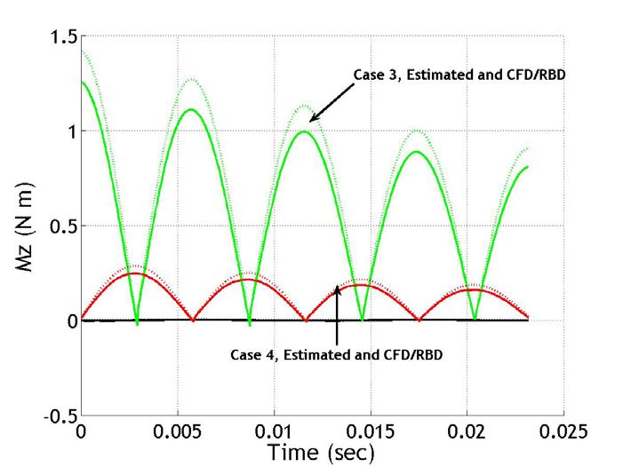
NOTICES

                                          Disclaimers

The findings in this report are not to be construed as an official Department of the Army position
unless so designated by other authorized documents.

Citation of manufacturer’s or trade names does not constitute an official endorsement or
approval of the use thereof.

DESTRUCTION NOTICE⎯Destroy this report when it is no longer needed. Do not return it to
the originator.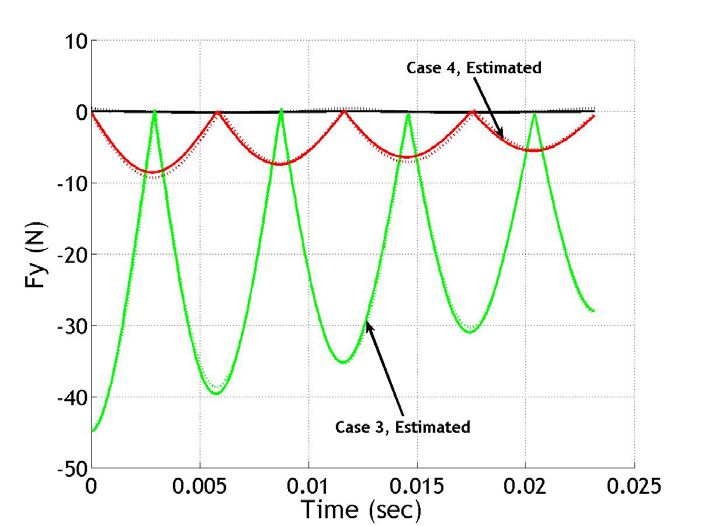
Army Research Laboratory
Aberdeen Proving Ground, MD 21005-5069

ARL-TR-4270                                                            September 2007

 Using Computational Fluid Dynamics-Rigid Body Dynamic
   (CFD-RBD) Results to Generate Aerodynamic Models
            for Projectile Flight Simulation

                               Mark Costello and Stephen Gatto
                                  Georgia Institute of Technology

                                              Jubaraj Sahu
                     Weapons and Materials Research Directorate, ARL

Approved for public release; distribution is unlimited.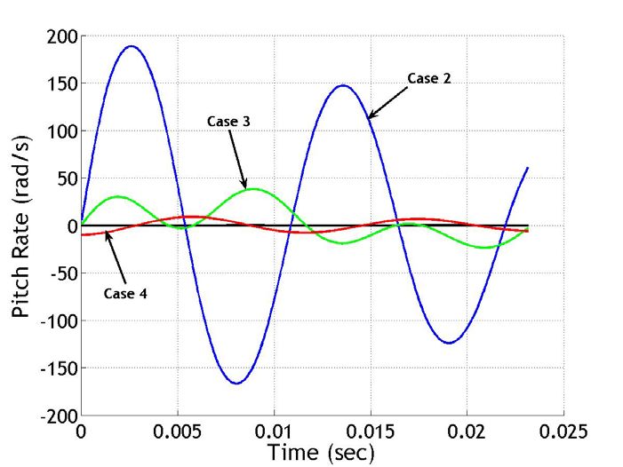
Form Approved
                          REPORT DOCUMENTATION PAGE                                                                                                             OMB No. 0704-0188
Public reporting burden for this collection of information is estimated to average 1 hour per response, including the time for reviewing instructions, searching existing data sources, gathering and maintaining the
data needed, and completing and reviewing the collection information. Send comments regarding this burden estimate or any other aspect of this collection of information, including suggestions for reducing the
burden, to Department of Defense, Washington Headquarters Services, Directorate for Information Operations and Reports (0704-0188), 1215 Jefferson Davis Highway, Suite 1204, Arlington, VA 22202-4302.
Respondents should be aware that notwithstanding any other provision of law, no person shall be subject to any penalty for failing to comply with a collection of information if it does not display a currently valid
OMB control number.
PLEASE DO NOT RETURN YOUR FORM TO THE ABOVE ADDRESS.
1. REPORT DATE (DD-MM-YYYY)                            2. REPORT TYPE                                                                       3. DATES COVERED (From - To)
   September 2007                                      Final                                                                                    January 2006 to August 2007
4. TITLE AND SUBTITLE                                                                                                                       5a. CONTRACT NUMBER

   Using Computational Fluid Dynamics-Rigid Body Dynamic (CFD-RBD)
                                                                                                                                            5b. GRANT NUMBER
   Results to Generate Aerodynamic Models for Projectile Flight Simulation
                                                                                                                                            5c. PROGRAM ELEMENT NUMBER

6. AUTHOR(S)                                                                                                                                5d. PROJECT NUMBER
                                                                                                                                                 622618AH80
  Mark Costello and Stephen Gatto (GIT); Jubaraj Sahu (ARL)
                                                                                                                                            5e. TASK NUMBER

                                                                                                                                            5f. WORK UNIT NUMBER

7. PERFORMING ORGANIZATION NAME(S) AND ADDRESS(ES)                                                                                          8. PERFORMING ORGANIZATION
U.S. Army Research Laboratory                                                                                                                 REPORT NUMBER
Weapons and Materials Research Directorate                                                                                                  ARL-TR-4270
Aberdeen Proving Ground, MD 21005-5069

9. SPONSORING/MONITORING AGENCY NAME(S) AND ADDRESS(ES)                                                                                     10. SPONSOR/MONITOR'S ACRONYM(S)

                                                                                                                                            11. SPONSOR/MONITOR'S REPORT
                                                                                                                                               NUMBER(S)

12. DISTRIBUTION/AVAILABILITY STATEMENT

    Approved for public release; distribution is unlimited.
13. SUPPLEMENTARY NOTES

14. ABSTRACT

A method to efficiently generate a complete aerodynamic description for projectile flight dynamic modeling is described. At
the core of the method is an unsteady, time-accurate computational fluid dynamics simulation that is tightly coupled to a rigid
projectile flight dynamic simulation. A set of short time snippets of simulated projectile motion at different Mach numbers is
computed and employed as baseline data. For each time snippet, aerodynamic forces and moments and the full rigid body state
vector of the projectile are known. With time-synchronized air loads and state vector information, aerodynamic coefficients can
be estimated with a simple fitting procedure. By inspecting the condition number of the fitting matrix, we can assess the
suitability of the time history data to predict a selected set of aerodynamic coefficients. The technique is exercised on an
exemplar fin-stabilized projectile with good results.

15. SUBJECT TERMS
    computational fluid dynamics; coupled CFD-RBD; high performance computing; rigid body dynamics
                                                                                        17. LIMITATION              18. NUMBER              19a. NAME OF RESPONSIBLE PERSON
16. SECURITY CLASSIFICATION OF:                                                         OF ABSTRACT                 OF PAGES                     Jubaraj Sahu
a. REPORT                 b. ABSTRACT                   c. THIS PAGE                                                                        19b. TELEPHONE NUMBER (Include area code)
                                                                                                SAR                         35
Unclassified              Unclassified                  Unclassified                                                                           410-306-0800
                                                                                                                                                                                Standard Form 298 (Rev. 8/98)
                                                                                                                                                                               Prescribed by ANSI Std. Z39.18

                                                                                                         ii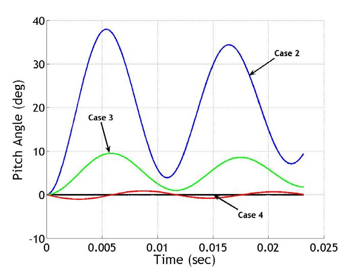
Contents

List of Figures                                             iv

List of Tables                                              iv

1.   Introduction                                            1

2.   Projectile CFD-RBD Simulation                          3

3.   Flight Dynamic Projectile Aerodynamic Model             6

4.   Projectile Aerodynamic Coefficient Estimation (PACE)    7

5.   Results                                                10

6.   Conclusions                                            21

7.   References                                             23

Distribution List                                           26

                                          iii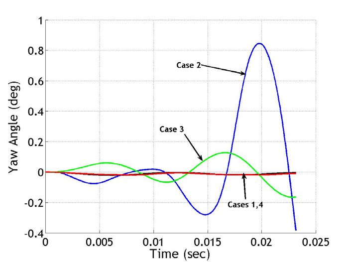
List of Figures
Figure 1. Reference frame and position definitions....................................................................... 4
Figure 2. Projectile orientation definitions. ................................................................................... 4
Figure 3. Unstructured mesh near the finned body...................................................................... 10
Figure 4. Velocity for the time snippets....................................................................................... 11
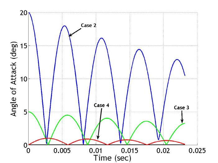
Figure 5. Aerodynamic angle of attack for the time snippets. ..................................................... 12
Figure 6. Roll rate for the time snippets. ..................................................................................... 12
Figure 7. Pitch rate for the time snippets. .................................................................................... 13
Figure 8. Euler pitch angle for the time snippets. ........................................................................ 13
Figure 9. Euler yaw angle for the time snippets. ......................................................................... 14
Figure 10. Estimated (dashed) and CFD-RBD (solid) body axis axial force (Fx) versus time. . 14
Figure 11. Estimated (dashed) and CFD-RBD (solid) normal force (Fy) versus time. ............... 15
Figure 12. Estimated (dashed) and CFD-RBD (solid) side force (Fz) versus time. .................... 15
Figure 13. Estimated (dashed) and CFD-RBD (solid) body axis rolling moment (Mx)
versus time. ........................................................................................................................... 16
Figure 14. Estimated (dashed) and CFD-RBD (solid) pitching moment (My) versus time. ....... 16
Figure 15. Estimated (dashed) and CFD-RBD (solid) yawing moment (Mz) versus time.......... 17
Figure 16. Zero yaw axial force coefficient versus Mach number. ............................................. 18
Figure 17. Yaw axial force coefficient versus Mach number...................................................... 18
Figure 18. Normal force coefficient versus Mach number. ......................................................... 19
Figure 19. Pitching moment coefficient versus Mach number. ................................................... 19
Figure 20. Roll damping moment coefficient versus Mach number. .......................................... 20
Figure 21. Pitch-damping moment coefficient versus Mach number.......................................... 20
Figure 22. Pitch-damping moment coefficient versus number of points per time snippet. ......... 21
List of Tables
Table 1. Time snippet initial conditions. ..................................................................................... 10
Table 2. Comparison of estimated aerodynamic coefficients and estimated coefficients at
Mach 3.0. .............................................................................................................................. 17
iv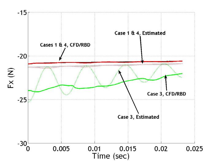
1. Introduction

Four basic methods to predict aerodynamic forces and moments on a projectile in atmospheric
flight are commonly used in practice: empirical methods, wind tunnel testing, computational fluid
dynamics (CFD) simulation, and spark range testing. Empirical methods have been found very
useful in conceptual design of projectiles where rapid and inexpensive estimates of aerodynamic
coefficients are needed. These techniques aerodynamically describe the projectile with a set of
geometric properties (diameter, number of fins, nose type, nose radius, etc) and catalog aerody-
namic coefficients of many different projectiles as a function of these features. These data are fit
to multivariable equations to create generic models for aerodynamic coefficients as a function of
these basic projectile geometric properties. The database of aerodynamic coefficients as a function
of projectile features is typically obtained from wind tunnel or spark range tests. Examples of this
approach to projectile aerodynamic coefficient estimation include missile DATCOM, PRODAS,
and AP981 (1 through 6). The advantage of this technique is that it is a general method applicable
to any projectile. However, it is the least accurate method of the four methods mentioned,
particularly for new configurations that fall outside the realm of projectiles used to form the basic
aerodynamic database.
Wind tunnel testing is often used during projectile development programs to converge on fine
details of the aerodynamic design of the shell (7, 8). In wind tunnel testing, a specific projectile
is mounted in a wind tunnel at various angles of attack with aerodynamic forces and moments
measured at various Mach numbers via a sting balance. Wind tunnel testing has the obvious
advantage of being based on direct measurement of aerodynamic forces and moments on the
projectile. It is also relatively easy to change the wind tunnel model to allow detailed parametric
effects to be investigated. The main disadvantage of wind tunnel testing is that it requires a wind
tunnel and is therefore modestly expensive. Furthermore, dynamic derivatives such as pitch and
roll damping as well as Magnus force and moment coefficients are difficult to obtain in a wind
tunnel and require a complex physical wind tunnel model.
Over the past couple of decades, tremendous strides have been made in the application of CFD to
predict aerodynamic loads on air vehicles including projectiles. These methods are increasingly
being used throughout the weapon development cycle including early in a program to create
relatively low cost estimates of aerodynamic characteristics and later in a program to supplement
and reduce expensive experimental testing. In CFD simulation, the fundamental fluid dynamic
equations are numerically solved for a specific configuration. The most sophisticated computer
codes are capable of unsteady time-accurate computations with the use of Navier-Stokes equations.
Examples of these tools include, for example, CFD++, Fluent, and Overflow-D. CFD is computa-
tionally expensive, requires powerful computers to obtain results in a reasonably timely manner,
  1
      DATCOM is not an acronym; PRODAS = Projectile Design and Analysis System; AP98 = AeroPrediction98.

                                                     1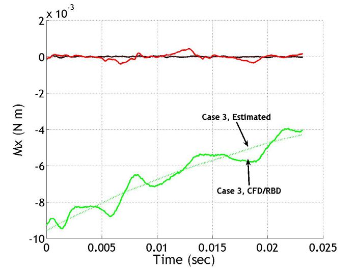
and requires dedicated engineering specialists to drive these tools (9 through 24). Spark range
aerodynamic testing has long been considered the gold standard for projectile aerodynamic
coefficient estimation. It is the most accurate method for obtaining aerodynamic data on a specific
projectile configuration. In spark range aerodynamic testing, a projectile is fired through an
enclosed building. At a discrete number of points during the flight of the projectile (< 30), the
state of the projectile is measured via spark shadowgraphs (25 through 29). The projectile state
data are subsequently fit to a rigid six-degree-of-freedom (6-DOF) projectile model with the use of
the aerodynamic coefficients as the fitting parameters (30, 31, 32). Although this technique is the
most accurate method for obtaining aerodynamic data on a specific projectile configuration, it is
usually the most expensive alternative, requires a spark range facility, and (strictly speaking) is
only valid for the specific projectile configuration tested.
Various researchers have used CFD to estimate aerodynamic coefficient estimation of projectiles.
Early work focused on Euler solvers applied to steady flow problems, while more recent work has
solved the Reynolds-averaged Navier-Stokes equations and large eddy simulation Navier-Stokes
equations for steady and unsteady conditions (9 through 24). For example, to predict pitch
damping, Weinacht prescribed projectile motion to mimic a typical pitch-damping wind tunnel test
in a CFD simulation to estimate the different components of the pitch-damping coefficient of a fin-
stabilized projectile (33). Excellent agreement between computed and measured pitch damping
was attained. Algorithm and computing advances have also led to the coupling of CFD codes to
projectile rigid body dynamics (RBD) codes to simulate free flight motion of a projectile in a time-
accurate manner. Aerodynamic forces and moments are computed with the CFD solver while the
free flight motion of the projectile is computed by the integration of the RBD equations of motion.
Sahu achieved excellent agreement between spark range measurements and a coupled CFD-RBD
approach for a fin-stabilized projectile (34). Projectile position and orientation at down-range
locations consistent with a spark range test were extracted from the output of the CFD-RBD
software to compute aerodynamic coefficients. Standard range reduction software was used for
this purpose with good agreement obtained when contrasted against sample spark range results.
The ability to accurately compute projectile aerodynamics in highly unsteady conditions has led to
the notion of “virtual wind tunnels” and “virtual fly-outs” where the simulation tools are used to
replicate a wind tunnel or spark range test.
Computation time for accurate coupled CFD-RBD simulation remains exceedingly high and does
not currently represent a practical method for typical flight dynamic analysis such as impact point
statistics (e.g., circular error probable) computation where thousands of “fly-outs” are required.
Furthermore, this type of analysis does not allow the same level of understanding of the inherent
underlying dynamics of the system that RBD analysis with aerodynamic coefficients yields.
However, the coupled CFD-RBD approach does offer an indirect way to rapidly compute the
aerodynamic coefficients needed for rigid 6-DOF simulation. During a time-accurate CFD-RBD
simulation, aerodynamic forces and moments and the full rigid body state vector of the projectile
are generated at each time step in the simulation (34). This means that aerodynamic forces,

                                                2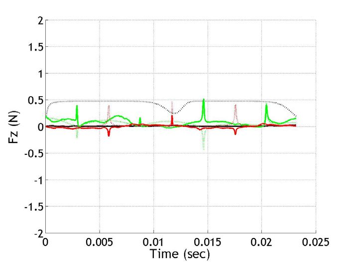
aerodynamic moments, position of the mass center, body orientation, translational velocity, and
angular velocity of the projectile are all known at the same time instant. With time-synchronized
air load and state vector information, the aero-dynamic coefficients can be estimated with a simple
fitting procedure. This report creates a method to efficiently generate a complete aerodynamic
model for a projectile in atmospheric flight with four short time histories at each Mach number of
interest with an industry standard time-accurate CFD-RBD simulation. The technique is exercised
on sample CFD-RBD data for a small fin-stabilized projectile. Parametric trade studies
investigating the required length of each time snippet as well as the required CFD accuracy are
reported.

2. Projectile CFD-RBD Simulation

The projectile CFD-RBD algorithm employed here combines a rigid 6-DOF projectile flight
dynamic model with a three-dimensional (3-D), time-accurate CFD simulation. The RBD dynamic
equations are integrated forward in time where aerodynamic forces and moments that drive the
motion of the projectile are computed via the CFD algorithm. The RBD projectile model allows
for three translational degrees of freedom and three rotational degrees of freedom. As shown in
figures 1 and 2, the I frame is attached to the ground while the B frame is fixed to the projectile
          G                                                         G       G
with the I B axis pointing out the nose of the projectile and the J B and K B unit vectors forming a
right-handed triad. The projectile state vector is comprised of the inertial position components of
the projectile mass center ( x, y, z ), the standard aerospace sequence Euler angles ( φ, θ, ψ ), the body
frame components of the projectile mass center velocity ( u, v, w ), and the body frame components
of the projectile angular velocity vector ( p, q, r ).

Both the translational and rotational dynamic equations are expressed in the projectile body
reference frame. The standard rigid projectile, body frame equations of motion are given by
equations 1 through 4.

                         ⎧ x& ⎫ ⎡cθ cψ      sφ sθ cψ − cφ sψ     cφ sθ cψ + sφ sψ ⎤ ⎧ u ⎫
                         ⎪ ⎪ ⎢                                                    ⎥⎪ ⎪
                         ⎨ y& ⎬ = ⎢ cθ sψ   sφ sθ sψ + cφ cψ     cφ sθ sψ − sφ cψ ⎥ ⎨ v ⎬           (1)
                         ⎪ z& ⎪ ⎢ − s                                             ⎥⎦ ⎪⎩ w ⎪⎭
                         ⎩ ⎭ ⎣ θ                  sφ cθ                cφ cθ

                                     ⎧φ& ⎫ ⎡1 sφ tθ             cφ tθ ⎤ ⎧ p ⎫
                                     ⎪ &⎪ ⎢                             ⎥⎪ ⎪
                                     ⎨θ ⎬ = ⎢0   cφ             − sφ ⎥ ⎨ q ⎬                        (2)
                                     ⎪ψ& ⎪ ⎢0 s / c            cφ / cθ ⎥⎦ ⎪⎩ r ⎪⎭
                                     ⎩ ⎭ ⎣     φ    θ

                                                       3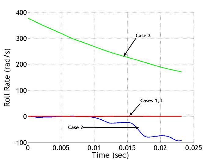
⎧ u& ⎫ ⎧ X / m ⎫ ⎡ 0 − r q ⎤ ⎧ u ⎫
         ⎪ ⎪ ⎪               ⎪ ⎢               ⎪ ⎪
         ⎨ v& ⎬ = ⎨ Y / m ⎬ − ⎢ r     0 − p⎥ ⎨ v ⎬        (3)
                                             ⎥
         ⎪ w& ⎪ ⎪ Z / m ⎪ ⎢ − q p        0 ⎥⎦ ⎪⎩ w ⎪⎭
         ⎩ ⎭ ⎩               ⎭ ⎣
    ⎧ p& ⎫          ⎡ ⎧ L ⎫ ⎡ 0 − r q ⎤ ⎧ p ⎫⎤
    ⎪ ⎪          −1 ⎢ ⎪      ⎪ ⎢                 ⎪ ⎪⎥
    ⎨ q& ⎬ = [I ] ⎢ ⎨ M ⎬ − ⎢ r       0 − p ⎥[I ]⎨ q ⎬⎥   (4)
                                            ⎥
    ⎪ r& ⎪          ⎢⎣ ⎪⎩ N ⎪⎭ ⎢⎣ − q p  0 ⎥⎦ ⎪⎩ r ⎪⎭⎥⎦
    ⎩ ⎭

Figure 1. Reference frame and position definitions.

   Figure 2. Projectile orientation definitions.

                              4
Note that the total applied force components ( X , Y , Z ) and moment components ( L, M , N )
contain contributions from weight and aerodynamics. The aerodynamic portion of the applied
loads in equations 3 and 4 is computed with the CFD simulation and passed to the RBD
simulation.
On the other hand, the CFD flow equations are integrated forward in time where the motion of the
projectile that drives flow dynamics are computed with the RBD algorithm. The complete set of
3-D time-dependent Navier-Stokes equations is solved in a time-accurate manner for simulation of
free flight. The commercially available code, CFD++, is used for the time-accurate unsteady CFD
simulations (35, 36). The basic numerical framework in the code contains unified grid, unified
physics, and unified computing features. The 3-D, time-dependent Reynolds-averaged Navier-
Stokes (RANS) equations are solved with the following finite volume equation.
∂
∂t V∫
WdV + ∫ ( F − G ) dA = ∫ HdV
V
(5)
in which W is the vector of conservative variables, F and G are the inviscid and viscous flux
vectors, respectively, H is the vector of source terms, V is the cell volume, and A is the surface
area of the cell face. A second order discretization is used for the flow variables and the turbulent
viscosity equation. The turbulence closure is based on topology-parameter-free formulations.
Two-equation higher order RANS turbulence models are used for the computation of turbulent
flows. These models are ideally suited to unstructured bookkeeping and massively parallel
processing because of their independence from constraints related to the placement of boundaries
and/or zonal interfaces.
A dual time-stepping approach is used to integrate the flow equations to achieve the desired time
accuracy. The first is an “outer” or global (and physical) time step that corresponds to the time
discretization of the physical time variation term. This time step can be chosen directly by the user
and is typically set to a value to represent 1/100 of the period of oscillation expected or forced in
the transient flow. It is also applied to every cell and is not spatially varying. An artificial or
“inner” or “local” time variation term is added to the basic physical equations. This time step and
corresponding “inner iteration” strategy is chosen to help satisfy the physical transient equations
to the desired degree. For the inner iterations, the time step is allowed to vary spatially. Also,
relaxation with multi-grid (algebraic) acceleration is employed to reduce the residues of the
physical transient equations. It is found that an order of magnitude reduction in the residues is
usually sufficient to produce a good transient iteration.
The projectile in the coupled CFD-RBD simulation, along with its grid, moves and rotates as the
projectile flies down range. Grid velocity is assigned to each mesh point. For a spinning and
yawing projectile, the grid speeds are assigned as if the grid were attached to the projectile and
spinning and yawing with it.
5In order to properly initialize the CFD simulation, two modes of operation for the CFD code are
used, namely, an uncoupled and a coupled mode. The uncoupled mode is used to initialize the
CFD flow solution while the coupled mode represents the final time accurate coupled CFD-RBD
solution. In the uncoupled mode, the RBD are specified. The uncoupled mode begins with a
computation performed in “steady state mode” with the grid velocities prescribed to account for
the proper initial position ( x0 , y0 , z0 ), orientation ( φ0 ,θ 0 ,ψ 0 ), and translational velocity ( u0 , v0 , w0 )
components of the complete set of initial conditions to be prescribed. After the steady state
solution is converged, the initial spin rate ( p0 ) is included and a new quasi-steady state solution
is obtained with time-accurate CFD. A sufficient number of time steps are performed so that the
angular orientation for the spin axis corresponds to the prescribed initial conditions. This quasi-
steady state flow solution is the starting point for the time-accurate coupled solution. For the
coupled solution, the mesh is translated back to the desired initial position ( x0 , y0 , z0 ) and the
remaining angular velocity initial conditions ( q0 , r0 ) are then added. In the coupled mode, the
aerodynamic forces and moments are passed to the RBD simulation which propagates the rigid
state of the projectile forward in time.
3. Flight Dynamic Projectile Aerodynamic Model
The applied loads in equations 3 and 4 contain contributions from projectile weight and body
aerodynamic forces and moments:
⎧ ⎫
⎪C X 0 + C X 2 (v 2 + w2 ) / V 2 ⎪
⎧X ⎫ ⎧ − sθ ⎫ ⎪ ⎪
⎪ ⎪ ⎪ ⎪ π 2 2 ⎪ pD ⎪ (6)
⎨ ⎬
Y = W ⎨ φ θ⎬
s c − ρV D ⎨ NA
C v / V − C YPA w / V ⎬
⎪Z ⎪ ⎪c c ⎪ 8 ⎪ 2V ⎪
⎩ ⎭ ⎩ φ θ⎭ ⎪ pD ⎪
⎪⎩CNA w / V + 2V CYPAv / V ⎭⎪
⎧ pD ⎫
⎪ CLDD + CLP ⎪
⎧L⎫ 2V
⎪ ⎪
⎪ ⎪ π 2 3⎪ w qD pD v ⎪
⎨ ⎬
M = ρV D ⎨ MA
C + C MQ + C NPA ⎬ (7)
⎪N ⎪ 8 ⎪ V 2V 2V V ⎪
⎩ ⎭ ⎪ v rD pD w⎪
⎪ −CMA V + 2V CMQ + 2V CNPA V ⎪
⎩ ⎭
The terms containing CYPA constitute the Magnus air load acting at the Magnus center of pressure
while the terms containing C X 0 , C X 2 , CNA define the steady load acting at the center of pressure.
The externally applied moment about the projectile mass center is composed of an unsteady
aerodynamic moment along with terms because the center of pressure and center of Magnus are
6not located at the mass center. The terms involving CMA account for the center of pressure being
located off the mass center while the terms involving CNPA account for the center of Magnus being
located off the mass center. The aerodynamic coefficients are all a function of local Mach number
which are typically handled through a table look-up scheme in projectile flight simulation codes.
4. Projectile Aerodynamic Coefficient Estimation (PACE)
The time-accurate coupled CFD-RBD simulation provides a full flow solution, including the
aerodynamic portion of the total applied force and moment ( X , Y , Z , L, M , N ) along with the full
state of the rigid projectile ( x, y, z , φ ,θ ,ψ , u, v, w, p, q, r ) at every time step in the solution for each
time snippet. Given a set of n short time histories (snippets) that each contain m time points, we
obtain a total of h = m * n time history data points for use in estimating the aerodynamic coef-
ficients: C X 0 , C X 2 , CNA , CYPA , CLDD , CLP , CMA , CMQ , CNPA . Note that for fin-stabilized projectile
configurations, the Magnus force and moment are usually sufficiently small so that CYPA and CNPA
are set to zero and removed from the fitting procedure to be described next.
Equations 6 and 7 represent the applied air loads on the projectile expressed in the projectile body
frame. Computation of the aerodynamic coefficients is aided by transformation of these equations
to the instantaneous aerodynamic angle of attack reference frame that rotates the projectile body
r
frame about the I B axis by the angle γ = tan −1 ( w / v ) .
⎧ ⎫
⎪C X 0 + C X 2 (v 2 + w2 ) / V 2 ⎪
⎡1 0 0 ⎤⎛⎧X ⎫ ⎧ − sθ ⎫ ⎞ ⎪ ⎪
8 ⎢ ⎥⎜⎪ ⎪ ⎪ ⎪⎟ ⎪ v 2 + w2 ⎪
− 2 2 ⎢
0 cγ sγ ⎥ ⎜ ⎨ Y ⎬ − W ⎨ sφ cθ ⎬ ⎟ = ⎨ CNA ⎬ (8)
πρV D V
⎢0 − sγ
⎣ cγ ⎥⎦ ⎜⎝ ⎪⎩ Z ⎭⎪ ⎪c c ⎪ ⎟ ⎪
⎩ φ θ ⎭⎠ ⎪
⎪
pD v + w 2 2 ⎪
⎪ CYPA ⎪
⎩ 2V V ⎭
⎧ pD ⎫
⎪ CLDD + CLP ⎪
⎪ 2V ⎪
⎡1 0 0⎤⎧ L ⎫ ⎪ ⎪
⎢ ⎥ ⎪ ⎪ ⎪ (vq + wr ) D pD v + w ⎪
2 2
8
2 3 ⎢
0 cγ sγ ⎥ ⎨ M ⎬ = ⎨ CMQ + CNPA ⎬ (9)
πρV D 2 v 2 + w2 V 2V V
⎢
⎣0 − sγ cγ ⎦⎥ ⎩⎪ N ⎭⎪ ⎪ ⎪
⎪ ⎪
⎪ (vr − wq ) D C − v + w C
2 2
⎪
⎪⎩ 2 v 2 + w2 V MQ V
MA
⎭⎪
Each time history data point provides a total of six equations given by the components of equations
8 and 9. The first component of equation 8 is gathered together for all time history data points to
7form equation 10. Likewise, the second and third components of equation 8 generate equations 11
and 12, respectively, while the first component of equation 9 constructs equation 13. Finally, the
second and third components of equation 9 are gathered together to form equation 14. Subscripts
on the projectile state vector and aerodynamics force and moment components represent the time
history data point.
⎧ 8 ⎫
2 2 ( 1
⎪ − X + W sin θ1 ) ⎪
⎡1 (v + w ) / V ⎤
2 2 2
πρV1 D
⎥ ⎧C X 0 ⎫ ⎪⎪ ⎪⎪
1 1 1
⎢
⎢ M M ⎨
⎥ C ⎬ = ⎨ M ⎬ (10)
⎢1 (vh2 + wh2 ) / Vh2 ⎥ ⎩ X 2 ⎭ ⎪ 8 ⎪
⎣ ⎦ ⎪− ( X + W sin θ ) ⎪
⎪⎩ πρVh D
h h
⎭⎪
2 2
⎧ 8 ⎫
⎡ v 2 + w2 / V ⎤ ⎪ − πρV 2 D 2 (Y1 cos γ 1 + Z1 sin γ 1 − W sin φ1 cos θ1 ) ⎪
⎢ 1 1 1
⎥ ⎪⎪ 1
⎪⎪
⎢ M ⎥ { NA } ⎨
C = M ⎬ (11)
⎢ 2 ⎥ ⎪ 8 ⎪
⎢⎣ vh + wh / Vh ⎥⎦ ( )
2
⎪− Y cos γ + Z sin γ − W sin φ cos θ ⎪
⎩⎪ πρVh D
h h h h h h
⎭⎪
2 2
⎡ p D v 2 + w2 ⎤ ⎧ 8 ⎫
⎢ 1 ⎥ ⎪ πρV 2 D 2 ( −Y1 sin γ 1 + Z1 cos γ 1 − W cos φ1 cos θ1 ) ⎪
−
1 1
⎢ ⎥
2
2V1
⎪ 1
⎪⎪
⎢ ⎥ {C } = ⎪
⎥ YPA ⎨ ⎬
M M (12)
⎢
⎢ p D v 2 + w2 ⎥ ⎪ 8 ⎪
⎢ h h h
⎥ ⎪ − ( −Y sin γ + Z cos γ − W cos φ cos θ ) ⎪
⎪
⎩ πρVh2 D 2
h h h h h h
⎪⎭
⎣⎢ ⎦⎥
2
2V h
⎡ p1 D ⎤ ⎧ 8L1 ⎫
⎢1 2V1 ⎥ ⎪ πρV 2 D 3 ⎪
⎢ ⎥ ⎧CLDD ⎫ ⎪⎪ 1
⎪⎪
⎢M M ⎥⎨ =
⎬ ⎨ M ⎬ (13)
⎢ ⎥ ⎩ CLP ⎭ ⎪
⎢1 ph D ⎥ 8Lh ⎪
⎪ ⎪
⎢⎣ 2Vh ⎥⎦ ⎪⎩ πρVh D ⎪⎭
2 3
8⎡ (v1q1 + w1r1 ) D p1 D v12 + w12 ⎤
⎢ 0 ⎥ ⎧ 8 ⎫
⎢ ⎥ ⎪ πρV 2 D 3 ( M 1 cos γ 1 + N1 sin γ 1 ) ⎪
2V1 v12 + w12 2V12
⎢ ⎥ ⎪ 1
⎪
⎢ v12 + w12 (v1r1 − w1q1 ) D ⎥ ⎪ 8 ⎪
⎢− 0 ⎥ ⎪ 2 3 (
− M 1 sin γ 1 + N1 cos γ 1 ) ⎪
⎢ V1 2V1 v12 + w12 ⎥ ⎧ CMA ⎫ ⎪ πρV1 D ⎪⎪
⎢ ⎥ ⎪C ⎪ = ⎪
⎢ M M M ⎥ ⎨ MQ ⎬ ⎨ M ⎬ (14)
⎢ ⎪ ⎪ ⎪ ⎪
(vh qh + wh rh ) D ph D vh2 + wh2 ⎥ ⎩CNPA ⎭ ⎪ 8
( γ + γ ) ⎪
⎢ ⎥ M cos N sin
⎢
0 2
⎥ ⎪ πρV 2 3
D
h h h h
⎪
2Vh vh2 + wh2 2Vh
⎪
h
⎪
⎢ ⎥ 8
⎢ vh2 + wh2 (vh rh − wh qh ) D ⎥ ⎪ ( − M sin γ + N cos γ ) ⎪
⎪⎩ πρVh D ⎭⎪
2 3 h h h h
⎢− 0 ⎥
⎢⎣ Vh 2Vh vh2 + wh2 ⎥⎦
Equations 10 through 14 represent a set of five uncoupled problems to solve for the different aero-
dynamic coefficients. To estimate the aerodynamic coefficients near a particular Mach number, a
set of n time accurate coupled CFD-RBD simulations are created over a relatively short time
period. Since an individual time snippet is over a short time period where the projectile state
variables does not change appreciably, it is critical that initial conditions for the different time
snippet be selected in an informed way so that the rank of each of the fitting matrices is maximal.
Properties of the fitting matrices, such as the rank or condition number, can be used as an indicator
of the suitability of the CFD-RBD simulation data to estimate the aerodynamic coefficients at the
target Mach number. Equation 10 is employed to estimate the zero yaw drag coefficient ( C X 0 ) and
the yaw drag coefficient ( C X 2 ). To minimize the condition number of this fitting matrix, both low
and high aerodynamic angle of attack time snippets are required. Equation 11 is used to compute
the normal force coefficient ( CNA ) and it requires time history data with a non-zero aerodynamic
angle of attack. Equation 12 is used to compute the Magnus force coefficient ( CYPA ) and it requires
time history data with both low and high roll rate and aerodynamic angle of attack. Equation 13 is
employed to estimate the fin cant roll coefficient ( CLDD ) along with the roll-damping coefficient
( CLP ). To minimize the condition number of this fitting matrix, both low and high roll rate time
snippets are required. Equation 14 is employed to estimate the pitching moment coefficient
( CMA ), the pitch-damping coefficient ( CMQ ), and the Magnus moment coefficient ( CNPA ). For
successful estimation of these coefficients, time history data with both low and high roll rate and
aerodynamic angle of attack as well as low and high aerodynamic angle of attack are required. To
meet all the requirements for successful estimation of all five sets of aerodynamic coefficients, four
time snippets are used, all with different initial conditions. Table 1 lists the four cases with launch
conditions. Notice that the set of time snippets contains a diverse set of initial conditions: zero
aerodynamic angle of attack and angular rates; high angle of attack and zero angular rates; low
angle of attack, high roll rate with other angular rates zero; zero angle of attack, high pitch rate with
other angular rates zero.
9Table 1. Time snippet initial conditions.
State Case 1 Case 2 Case 3 Case 4
x (m) 0 0 0 0
y (m) 0 0 0 0
z (m) 0 0 0 0
Phi (deg) 0 0 0 0
Theta (deg) 0 0 0 0
Psi (deg) 0 0 0 0
V(m/s) 1032 1032 1032 1032
v (m/s) 0 0 0 0
w (m/s 0 -352.5 -90 0
p (rad/s) 0 0 377 0
q (rad/s) 0 0 0 -10
r (rad/s) 0 0 0 0
Alpha (deg) 0 20 5 0
For flight dynamic simulation, aerodynamic coefficients are required at a set of Mach numbers
that covers the intended spectrum of flight conditions for the round. If aerodynamic coefficients
are estimated at k different Mach numbers, then a total of l = k * n time snippets must be
generated to construct the entire aerodynamic database for flight simulation purposes.
5. Results
In order to exercise the method developed, a generic finned projectile is considered. A sketch of
the projectile is shown in figure 3. The projectile has the following geometric and mass properties:
length = 0.1259 m, reference diameter = 0.013194 m, mass = 0.0484 kg, mass center location from
base = 0.0686 m, roll inertia = 0.74E-06 kg m2, pitch inertia = 0.484E-04 kg m2.
Figure 3. Unstructured mesh near the finned body.
Figures 4 through 9 present projectile state trajectories for each of the four time snippets. Each
time snippet is 0.023 second and contains 50 points, leading to an average output time step of
0.0004. The initial conditions for each of the time snippets are shown in table 1. These four
snippets create time history data at low and high angle of attack, roll rate, and pitch rate needed for
accurate aerodynamic coefficient estimation. Notice that Cases 2 and 3 have notably more drag
because of the high angle of attack launch conditions. Case 3 is launched with relatively high roll
10rate compared to all other cases. Case 4 generates roll rate toward the end of the time snippet
because of high angle of attack roll-pitch coupling. Significant oscillations in Euler pitch angle are
created in Case 2 with some cross-coupling response exhibited in Euler yaw angle. Figures 10
through 15 plot aerodynamic forces and moments in the local angle of attack reference frame
defined for Cases 1, 3, and 4 since these cases are the primary ones used to estimate the coef-
ficients. For all cases, the axial force oscillates from -20 N to -25 N. There exists a slight bias
between the CFD-RBD and estimated data of about 0.5 N for low angle of attack time snippets.
For moderately high angles of attack (Case 3), the estimated data also oscillate with a much higher
amplitude than the CFD-RBD data, indicating that CX2 is estimated larger than the CFD-RBD
suggests. The normal force time snippets agree well between the CFD-RBD and estimated data
for all time snippets. For the sample finned projectile, side force and out-of-plane moment are
generally small (< 0.5 N, 0.05 Newton meters [Nm]) because of a negligibly small Magnus force
and moment. The CFD-RBD and estimated data agree reasonably well but certainly do not over-
lie one another. The only time snippet that creates notable rolling moment is Case 3 which is
launched with an initial roll rate of 377 rad/sec. Notice that the estimated data smoothly go
through the CFD-RBD data which oscillate in a slightly erratic manner. The in-plane moment
(Mz) agrees reasonably well for both the CFD-RBD and estimated data. The results shown in
figures 4 through 15 are typical for all Mach numbers. The overall observation from the data is
that the estimated aerodynamic model fits the CFD-RBD data well, with the notable exception of
axial force where a bias between the two is exhibited.
Figure 4. Velocity for the time snippets.
11Figure 5. Aerodynamic angle of attack for the time snippets.
Figure 6. Roll rate for the time snippets.
12Figure 7. Pitch rate for the time snippets.
Figure 8. Euler pitch angle for the time snippets.
13Figure 9. Euler yaw angle for the time snippets.
Figure 10. Estimated (dashed) and CFD-RBD (solid) body axis axial force (Fx)
versus time.
14Figure 11. Estimated (dashed) and CFD-RBD (solid) normal force (Fy) versus time.
Figure 12. Estimated (dashed) and CFD-RBD (solid) side force (Fz) versus time.
15Figure 13. Estimated (dashed) and CFD-RBD (solid) body axis rolling moment (Mx)
versus time.
Figure 14. Estimated (dashed) and CFD-RBD (solid) pitching moment (My) versus time.
16Figure 15. Estimated (dashed) and CFD-RBD (solid) yawing moment (Mz) versus time.
The sample projectile investigated in this report has been fired in a spark range at Mach 3.0 with
aerodynamic coefficients computed via conventional aerodynamic range reduction. Table 2
presents a comparison of aerodynamic coefficients obtained from spark range testing and sub-
sequent coefficients obtained with the method described here. Notice that most aerodynamic
coefficients such as CX0, CNA, and CMA are in reasonably good agreement with the test data. Axial
force yaw drag and roll damping are both different by ~20%, while pitch damping is different by
~40%. Differences in the spark range and estimated coefficients can be attributed to several
factors, such as inaccuracies in the CFD-RBD solution, the manner in which the spark range
data were reduced, and inaccurate estimation because of insufficiently rich data.
Table 2. Comparison of estimated aerodynamic coefficients and estimated coefficients at Mach 3.0.
Spark Range CFD-RBD – Percent Difference
Data – Spark PACE Between Coefficients
Range Reduction
Zero Yaw Axial Force Coefficient, CX0 0.221 0.238 7.1 to 7.7
Yaw Axial Force Coefficient, CX2 5.0 5.9 15.0 to 18.0
Normal Force Coefficient Derivative, 5.83 5.64 3.2 to 3.3
CNA
Pitching Moment Coefficient Derivative, -12.6 -13.82 8.8 to 9.7
CMA
Pitch-Damping Moment Coefficient, CMQ -196 -134 31.6 to 46.3
Roll-Damping Moment Coefficient, CLP -2.71 -3.37 19.6 to 24.4
CFD-RBD data were generated at six different Mach numbers ranging from 1.5 to 4.0. The
estimation algorithm discussed was used to compute a complete set of aerodynamic coefficients
across its Mach range. These results are provided in table 3 with plots of the individual aerody-
17namic coefficients given in figures 16 through 21. With the exception of CX2, the steady aero-
dynamic coefficients are smooth and follow typical trends for variation in Mach number. The yaw
drag coefficient, CX2, however, is somewhat erratic with a low value of 0.21 at Mach 1.5 followed
by a steady rise until Mach 3.5. Pitch damping decreases with Mach number, as would be
expected for a fin-stabilized projectile beyond Mach 1.0. However, roll damping steadily increases
until Mach 4.0 when in drops off notably.
Figure 16. Zero yaw axial force coefficient versus Mach number.
Figure 17. Yaw axial force coefficient versus Mach number.
18Figure 18. Normal force coefficient versus Mach number.
Figure 19. Pitching moment coefficient versus Mach number.
19Figure 20. Roll damping moment coefficient versus Mach number.
Figure 21. Pitch-damping moment coefficient versus Mach number.
20In order to investigate convergence of the estimation procedure, the number of points used per time
snippet was varied from a single point per time snippet to 50 points per time snippet. Of all the
coefficients, the pitch-damping coefficient generally required the most number of points to
converge. Figure 22 plots estimated pitch-damping coefficient versus the number of points per
time snippet. For this aerodynamic coefficient, convergence is reached after about 50 points per
time snippet. The points extracted from each time snippet are from the beginning of the time
history and are not evenly extracted over the entire time history.
Figure 22. Pitch-damping moment coefficient versus number of points per time snippet.
6. Conclusions
With a time-accurate CFD simulation that is tightly coupled to an RBD simulation, a method to
efficiently generate a complete aerodynamic description for projectile flight dynamic modeling is
described. A set of n short time snippets of simulated projectile motion at m different Mach
numbers is computed and employed as baseline data. The combined CFD-RBD analysis computes
time-synchronized air loads and projectile state vector information, leading to a straightforward
fitting procedure to obtain the aerodynamic coefficients. The estimation procedure decouples into
five sub-problems that are each solved via linear least squares. The method has been applied to a
sample supersonic finned projectile. Overall, the results are encouraging. A comparison of spark
range obtained aerodynamic coefficients with the estimation method presented here at Mach 3
exhibits good agreement within 10% for CX0, CNA, and CMA; agreement within 20% for CX2 and
CLP; and poor agreement within 40% for CMQ. Convergence of the aerodynamic coefficients is a
21strong function of the number of points in each time snippet with pitch damping generally requiring
the most number of points for convergence. This technique reported here provides a promising
new means for the CFD analyst to predict aerodynamic coefficients for flight dynamic simulation
purposes. It can easily be extended to flight dynamic modeling of different control effectors,
provided that accurate CFD-RBD time simulation is possible and an aerodynamic coefficient
expansion is defined which includes the effect of the control mechanism.
227. References
1. Sun, J.; Cummings, R. Evaluation of Missile Aerodynamic Characteristics Using Rapid
Prediction Techniques. Journal of Spacecraft and Rockets 1984, 21 (6), 513-520.
2. Moore, F. The 2005 Version of the Aeroprediction Code (AP05). AIAA 2004-4715, AIAA
Atmospheric Flight Mechanics Conference, Providence, Rhode Island, 2004.
3. Sooy, T.; Schmidt, R. Aerodynamic Predictions, Comparisons, and Validations Using
Missile DATCOM and Aeroprediction 98. AIAA-2004-1246, AIAA Aerospace Sciences
Meeting and Exhibit, Reno, Nevada, 2004.
4. Simon, J.; Blake, W. Missile DATCOM – High Angle of Attack Capabilities. AIAA-1999-
4258, AIAA Atmospheric Flight Mechanics Conference, Portland, Oregon, 1999.
5. Neely, A.; Auman, I. Missile DATCOM Transonic Drag Improvements for Hemispherical
Nose Shapes. AIAA-2003-3668, AIAA Applied Aerodynamics Conference, 2003.
6. Blake, W. Missile DATCOM – 1997 Status and Future Plans. AIAA-1997-2280, AIAA
Applied Aerodynamics Conference, Atlanta, Georgia, 1997.
7. Dupuis, A.; Berner, C. Wind Tunnel Tests of a Long Range Artillery Shell Concept. AIAA-
2002-4416, AIAA Atmospheric Flight Mechanics Conference, Monterey, California, 2002.
8. Berner, C.; Dupuis, A. Wind Tunnel Tests of a Grid Fin Projectile Configuration. AIAA-
2001-0105, AIAA Aerospace Sciences Meeting, Reno, Nevada, 2001.
9. Evans, J. Prediction of Tubular Projectile Aerodynamics Using the ZUES Euler Code.
Journal of Spacecraft and Rockets 1989, 26 (5), 314-321.
10. Sturek, W.; Nietubicz, C.; Sahu, J.; Weinacht, P. Applications of Computational Fluid
Dynamics to the Aerodynamics of Army Projectiles. Journal of Spacecraft and Rockets
1994, 31 (2), 186-199.
11. Nusca, M.; Chakravarthy, S.; Goldberg, U. Computational Fluid Dynamics Capability for
the Solid-Fuel Ramjet Projectile. Journal of Propulsion and Power 1990, 6 (3).
12. Silton, S. Navier-Stokes Computations for a Spinning Projectile from Subsonic to
Supersonic Speeds. Journal of Spacecraft and Rockets 2005, 42 (2), 223-231.
13. DeSpirito, J.; Vaughn, M.; Washington, D. Numerical Investigation of Canard-Controlled
Missile with Planar Grid Fins. Journal of Spacecraft and Rockets 2003, 40 (3), 363-370.
14. Sahu, J. Numerical Computations of Transonic Critical Aerodynamic Behavior. AIAA
Journal May 1990, 28 (5), 807-816.
2315. Weinacht, P. Navier-Stokes Prediction of the Individual Components of the Pitch Damping
Sum. Journal of Spacecraft and Rockets 1998, 35 (5), 598-605.
16. Guidos, B.; Weinacht, P.; Dolling, D. Navier-Stokes Computations for Pointed, Spherical,
and Flat Tipped Shells at Mach 3. Journal of Spacecraft and Rockets 1992, 29 (3), 305-311.
17. Sahu, J.; Nietubicz, C. J. Application of Chimera Technique to Projectiles in Relative
Motion. Journal of Spacecraft & Rockets Sept-Oct 1995.
18. Park, S.; Kwon, J. Navier-Stokes Computations of Stability Derivatives for symmetric
Projectiles. AIAA-2004-0014, AIAA Aerospace Sciences Meeting, Reno, Nevada, 2004.
19. Sahu, J. Numerical Simulations of Supersonic Flow over an Elliptic-Section Projectile with
Jet-Interaction. AIAA Paper No. 2002-3260, St. Louis, MO, 24-27 June 2002.
20. Qin, N.; Ludlow, K.; Shaw, S.; Edwards, J.; Dupuis, A. Calculation of Pitch Damping for a
Flared Projectile. Journal of Spacecraft and Rockets 1997, 34 (4), 566-568.
21. Weinacht, P. Coupled CFD/GN&C Modeling for a Smart Material Canard Actuator.
AIAA-2004-4712, AIAA Atmospheric Flight Mechanics Conference, Providence, Rhode
Island, 2004.
22. Park, S.; Kim, Y.; Kwon, J. Prediction of Dynamic Damping Coefficients Using Unsteady
Dual Time Stepping Method. AIAA-2002-0715, AIAA Aerospace Sciences Meeting, Reno,
Nevada, 2002.
23. DeSpirito, J.; Heavey, K. CFD Computation of Magnus Moment and Roll-Damping
Moment of a Spinning Projectile. AIAA-2004-4713, AIAA Atmospheric Flight Mechanics
Conference, Providence, Rhode Island, 2004.
24. Sahu, J.; Heavey, K. R. Unsteady CFD Modeling of Micro-Adaptive Flow Control for an
Axisymmetric Body. International Journal of Computational Fluid Dynamics April-May
2006, 5.
25. Garon, K.; Abate, G.; Hathaway, W. Free-Flight Testing of a Generic Missile with MEMs
Protuberances. AIAA -2003-1242, AIAA Aerospace Sciences Meeting, Reno, Nevada, 2003.
26. Kruggel, B. High Angle of Attack Free Flight Missile Testing. AIAA-1999-0435, AIAA
Aerospace Sciences Meeting, Reno, Nevada, 1999.
27. Danberg, J.; Sigal, A.; Clemins, I. Aerodynamic Characteristics of a Family of Cone-
Cylinder-Flare Projectiles. Journal of Spacecraft and Rockets 1990, 27 (4).
28. Dupuis, A. Free-Flight Aerodynamic Characteristics of a Practice Bomb at Subsonic and
Transonic Velocities. AIAA-2002-4414, AIAA Atmospheric Flight Mechanics Conference,
Monterey, California, 2002.
2429. Abate, G.; Duckerschein, R.; Hathaway, W. Subsonic/transonic Free-Flight Tests of a
Generic Missile with Grid Fins. AIAA-2000-0937, AIAA Aerospace Sciences Meeting,
Reno, Nevada, 2000.
30. Chapman, G.; Kirk, D. A Method for Extracting Aerodynamic Coefficients from Free-Flight
Data. AIAA Journal 1970, 8 (4), 753-758.
31. Abate, G.; Klomfass, A. Affect upon Aeroballistic Parameter Identification from Flight Data
Errors. AIAA Aerospace Sciences Meeting, Reno, Nevada, 2005.
32. Abate, G.; Klomfass, A. A New Method for Obtaining Aeroballistic Parameters from Flight
Data. Aeroballistic Range Association Meeting, Freiburg, Germany, 2004.
33. Weinacht, P.; Sturek, W.; Schiff, L. Projectile Performance, Stability, and Free-Flight
Motion Prediction Using Computational Fluid Dynamics. Journal of Spacecraft and Rockets
2004, 41 (2), 257-263.
34. Sahu, J. Time-Accurate Numerical Prediction of Free-Flight Aerodynamics of a Finned
Projectile. AIAA-2005-5817, AIAA Atmospheric Flight Mechanics Conference, San
Francisco, California, 2005.
35. Peroomian, O.; Chakravarthy, S.; Goldberg, U. A ‘Grid-Transparent’ Methodology for
CFD. AIAA Paper 97-07245, 1997.
36. Peroomian, O.; Chakravarthy, S.; Palaniswamy, S.; Goldberg, U. Convergence Acceleration
for Unified-Grid Formulation Using Preconditioned Implicit Relaxation. AIAA Paper 98-
0116, 1998.
37. Abate, G.; Klomfass, A. Affect upon Aeroballistic Parameter Identification from Flight Data
Errors. AIAA-2005-0439, AIAA Aerospace Sciences Meeting, Reno, Nevada, 2005.
25NO. OF NO. OF
COPIES ORGANIZATION COPIES ORGANIZATION
1 DEFENSE TECHNICAL 1 ATK ORDNANCE SYS
(PDF INFORMATION CTR ATTN B BECKER
ONLY) DTIC OCA MN07 MW44
8725 JOHN J KINGMAN RD 4700 NATHAN LANE N
STE 0944 PLYMOUTH MN 55442
FORT BELVOIR VA 22060-6218
1 SCIENCE APPLICATIONS INTL CORP
1 US ARMY RSRCH DEV & ENGRG CMD ATTN J NORTHRUP
SYSTEMS OF SYSTEMS 8500 NORMANDALE LAKE BLVD
INTEGRATION SUITE 1610
AMSRD SS T BLOOMINGTON MN 55437
6000 6TH ST STE 100
FORT BELVOIR VA 22060-5608 3 GOODRICH ACTUATION SYSTEMS
ATTN T KELLY P FRANZ
1 DIRECTOR J CHRISTIANA
US ARMY RESEARCH LAB 100 PANTON ROAD
IMNE ALC IMS VERGENNES VT 05491
2800 POWDER MILL RD
ADELPHI MD 20783-1197 2 ARROW TECH ASSOC
ATTN W HATHAWAY J WHYTE
1 DIRECTOR 1233 SHELBURNE RD STE D8
US ARMY RESEARCH LAB SOUTH BURLINGTON VT 05403
AMSRD ARL CI OK TL
2800 POWDER MILL RD 1 KLINE ENGINEERING CO INC
ADELPHI MD 20783-1197 ATTN R W KLINE
27 FREDON GREENDEL RD
2 DIRECTOR NEWTON NJ 07860-5213
US ARMY RESEARCH LAB
AMSRD ARL CI OK T 1 GEORGIA INST TECH
2800 POWDER MILL RD DEPT AEROSPACE ENGR
ADELPHI MD 20783-1197 ATTN M COSTELLO
270 FERST STREET
1 AEROPREDICTION INC ATLANTA GA 30332
F MOORE
9449 GROVER DRIVE, STE 201 1 AIR FORCE RSRCH LAB
KING GEORGE VA 22485 AFRL/MNAV
ATTN G ABATE
1 UNIV OF TEXAS AT ARLINGTON 101 W EGLIN BLVD STE 333
MECH & AEROSPACE ENGINEERING DEPT EGLIN AFB FL 32542-6810
ATTN J C DUTTON
BOX 19018 1 US ARMY RDECOM ARDEC
500 W FIRST ST ATTN AMSRD AAR AEM A G MALEJKO
ARLINGTON TX 76019-0018 BLDG 95
PICATINNY ARSENAL NJ 07806-5000
2 ATK TACTICAL SYSTEMS DIV
ALLEGANY BALLISTICS LAB 2 US ARMY ARDEC
ATTN D J LEWIS J S OWENS ATTN AMSRD AAR AEP E D CARLUCCI
210 STATE ROUTE 956 ATTN AMSRD AAR AEP E I MEHMEDAGIC
ROCKET CENTER WV 26726 BLDG 94
PICATINNY ARSENAL NJ 07806-5000
1 ATK ADVANCED WEAPONS DIV
ATTN R H DOHRN 1 US ARMY TACOM ARDEC
MN06-1000 ATTN AMSRD AAR AEP E C KESSLER
4600 NATHAN LANE N BLDG 3022
PLYMOUTH MN 55442 PICATINNY ARSENAL NJ 07806-5000
26NO. OF
COPIES ORGANIZATION
1 APM SMALL & MED CALIBER AMMO
OPM MAS
ATTN SFAE AMO MAS SMC
R KOWALSKI
BLDG 354
PICATINNY ARSENAL NJ 07806-5000
3 US ARMY AMRDEC
ATTN AMSAM RD SS AT L AUMAN
R W KRETZSHMAR
E VAUGHN
REDSTONE ARSENAL AL 35898-5000
ABERDEEN PROVING GROUND
1 DIRECTOR
US ARMY RSCH LABORATORY
ATTN AMSRD ARL CI OK (TECH LIB)
BLDG 4600
18 DIR USARL
AMSRD WM
J SMITH
AMSRD WM B
M ZOLTOSKI
AMSRD WM BA
D LYON
AMSRD WM BC
P PLOSTINS
I CELMINS
M CHEN
J DESPIRITO
B GUIDOS
K HEAVEY
J SAHU
S SILTON
P WEINACHT
F FRESCONI
M BUNDY
G COOPER
B HOWELL
AMSRD WM BD
B FORCH
AMSRD WM BF
J NEWILL
S WILKERSON
H EDGE
27FOREIGN ADDRESSES
1 DSTL BEDFORD
T BIRCH
BLDG 115 RM 125
BEDFORD TECHNOLOGY PARK
BEDFORD
MK44 2FQ
UK
2 DEFENCE RESEARCH AND
DEVELOPMENT CANADA
VALCARTIER
F LESAGE
E FOURNIER
2459 PIE-XI BLVD NORTH
VAL BELAIR QC G3J1X5
CANADA
28You can also read