Masterton winter wood-smoke survey, 2018 - Greater ...
←
→
Page content transcription
If your browser does not render page correctly, please read the page content below
Masterton winter wood-
smoke survey, 2018

Tamsin Mitchell
Environmental Science Department

For more information, contact the Greater Wellington Regional Council:
Wellington                     Masterton                                 GW/ESCI-T-18/167
PO Box 11646                   PO Box 41
                                                                         March 2019
T 04 384 5708                  T 04 384 5708
F 04 385 6960                  F 06 378 2146
www.gw.govt.nz                 www.gw.govt.nz                            www.gw.govt.nz
                                                                         info@gw.govt.nz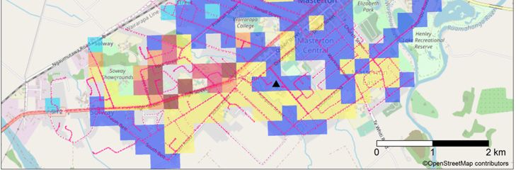
Report prepared by:                 T Mitchell            Senior Environmental
                                                          Scientist, Air Quality

Report reviewed by:                 R Uys                 Senior Terrestrial
                                                          Ecologist

Report approved for release by:     L Baker               Manager, Environmental
                                                          Science

                                                                                      Date: March 2019

 DISCLAIMER
 This report has been prepared by Environmental Science staff of Greater Wellington Regional Council (GWRC) and as
 such does not constitute Council policy.
 In preparing this report, the authors have used the best currently available data and have exercised all reasonable skill
 and care in presenting and interpreting these data. Nevertheless, GWRC does not accept any liability, whether direct,
 indirect, or consequential, arising out of the provision of the data and associated information within this report.
 Furthermore, as GWRC endeavours to continuously improve data quality, amendments to data included in, or used in
 the preparation of, this report may occur without notice at any time.
 GWRC requests that if excerpts or inferences are drawn from this report for further use, due care should be taken to
 ensure the appropriate context is preserved and is accurately reflected and referenced in subsequent written or verbal
 communications. Any use of the data and information enclosed in this report, for example, by inclusion in a subsequent
 report or media release, should be accompanied by an acknowledgement of the source.
 The report may be cited as:
 Mitchell T. 2019. Masterton winter wood smoke survey, 2018. Greater Wellington Regional Council, Publication No.
 GW/ESCI-T-18/167, Wellington.
Executive summary
The Masterton urban area experiences numerous high particle air pollution days
(measured as PM2.5) during the winter months when emissions from wood burning for
home heating coincide with calm and cold weather conditions. To better understand
patterns in wood smoke emissions, a vehicle containing a “SmokeTrak” monitoring
instrument was driven around Masterton over several winter evenings in June and July
2018.

These mobile monitoring results were used to map wood smoke levels across the
Masterton urban area. The maps show that levels of PM2.5 from wood smoke varied
considerably, with the highest concentrations found later in the evening, after 10 pm, in
the low-lying suburbs of Masterton East, Lansdowne and Solway South. Concentrations
of PM2.5 in these areas were likely higher than those measured at the GWRC Masterton
East monitoring station over the same time period. The lowest concentrations were
found outside the main urban area and at higher elevations in Lansdowne.

The mobile survey was carried out by GWRC and Masterton District Council as a first
step towards identifying areas with high wood smoke that could potentially receive
targeted education and assistance to reduce emissions of fine particles from wood
smoke.
Contents
Executive summary                                                              i

1.      Introduction                                                           1

2.      Background                                                            2
2.1     Study location                                                        2
2.2     Wood-burner operation and particle emissions                          3
2.3     PM2.5 concentrations from home heating                                4
2.3.1   Daily winter air quality profile measured at air quality monitoring
        stations                                                               4
2.3.2   Wood-burner use                                                        4
2.3.3   Impact of weather patterns and terrain                                 5

3.      Objectives                                                             7

4.      Methodology                                                           8
4.1     Car-based monitoring                                                  8
4.2     Sampling route                                                        9
4.3     Data processing and GIS analysis                                      9

5.      Results and discussion                                                11
5.1     Summary of SmokeTrak measurements                                     11
5.2     ‘Smokiness’ of the sampling nights                                    12
5.3     Time variation in wood smoke measurements                             14
5.4     Wood smoke maps                                                       14
5.4.1   SmokeTrak 5-second averages                                           14
5.4.2   SmokeTrak grid cell averages                                          15
5.4.3   SmokeTrak grid cell ratio to fixed monitoring station                 15
5.4.4   Limitations                                                           21

6.      Conclusion                                                            22

Acknowledgements                                                              23

References                                                                    24

Appendix A1: Co-location relationship – SmokeTrak and air quality
      monitoring station PM2.5 measurements                                   26

Appendix A2: GPS-recorded measurements of altitude along
      monitoring route                                                        28

Appendix A3: Masterton SmokeTrak measurements by sample date                  29

Appendix A4: Masterton SmokeTrak measurements by hour                         30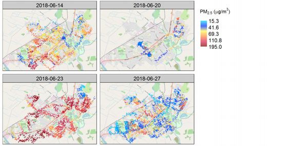
Masterton winter wood-smoke survey, 2018

1.   Introduction
     Masterton (Whakaoriori) is a rural town situated in the Upper Ruamahānga
     valley which is prone to air pollution episodes. These arise from the use of
     solid fuels for home heating during the winter months. The Masterton urban
     airshed is currently designated as a “polluted airshed” under the National
     Environmental Standard for Air Quality (NES-AQ). This is due to the multiple
     days per year when the PM10 24-hour average of 50 µg/m3 is exceeded. The
     NES-AQ requires the number of exceedances to be reduced to three per year
     by 1 September 2016 and then to one per year by 1 September 2020. The 1
     September 2016 target was not met.

     Recently the Government has signalled their intention to review the NES-AQ
     with a view to adopting a PM2.5 standard. Whilst, PM2.5 is a subset of PM10, it
     is more strongly associated with adverse health effects than PM10 and is a
     better indicator of combustion sources such as wood or coal burning. Over the
     past five years (2014 to 2018) air quality in Masterton failed to meet the World
     Health Organization 24-hour guideline for PM2.5 of 25 µg/m3 (World Health
     Organization 2006).

     Figure 1.1: Size of PM10 and PM2.5 particles compared to a strand of hair and to
     fine beach sand (Ministry for the Environment)

     The purpose of this study was to investigate the spatial variation of PM2.5 at a
     fine scale across the Masterton urban area to determine whether there are
     persistent areas of high wood-smoke particle emissions. These areas could then
     be targeted for assistance and/or education to reduce local emissions. It is
     thought that high emitting wood burners have a disproportionate impact on air
     quality and therefore reducing ‘hot spots’ of high air pollution may reduce
     exposure for the whole community (McGreevy & Barnes 2016).

                                                                                      PAGE 1 OF 30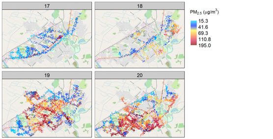
Masterton winter wood-smoke survey, 2018
2. Background
2.1 Study location
Masterton (Whakaoriori) is a rural town situated in the Upper Ruamahānga
valley (Figure 2.1) with approximately 20,000 residents. Masterton’s winters
are cooler on average and less windy than other parts of the Wellington region
(Chappell 2014).
Air quality is currently monitored at two fixed stations, Masterton West and
Masterton East (Figure 2.1). Masterton West is the long-term station that
measures long-term average air quality trends, while Masterton East is located
to measure the highest concentrations of particles (PM10) as required by the
NES-AQ. The stations are named after the Census Area Units that they are
located in. We do not know how well these stations represent unmonitored
parts of Masterton and whether there are persistent localised ‘hot spots’ of
elevated wood smoke in other locations around Masterton. Understanding the
variation in wood-smoke dispersion across the town provides a starting point
for identifying neighbourhoods that could benefit from targeted assistance to
improve air quality, both in their own neighbourhoods and in down-slope areas
that they might be affecting.
Figure 2.1: Map showing location of Masterton in the Upper Ruamahānga valley
and location of current fixed monitoring stations
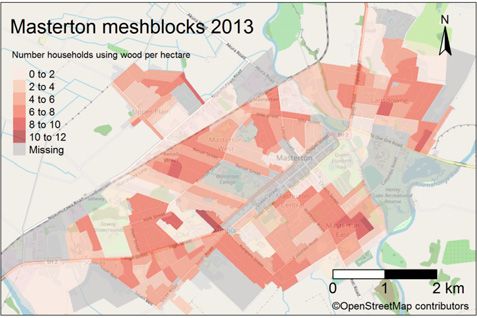
The majority of Masterton’s households (around 68%) burn wood for home
heating during the winter months and it is estimated that there are about 5,000
wood-burners in use (Figure 2.2, Statistics NZ 2013). Being able to affordably
heat your home is important for health and wellbeing. Firewood, especially if
self-collected, may cost less than electricity or gas for the same amount of heat
provided.
PAGE 2 OF 30 MASTERTON WOOD SMOKE SURVEY 2018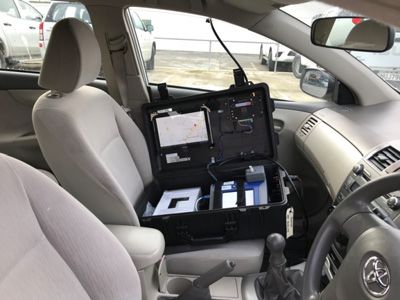
Masterton winter wood-smoke survey, 2018

                Figure 2.2: Density of wood-burning households per hectare by mesh block
                (Statistics NZ 2013)

                The downside of burning wood is that the smoke emitted contains fine particles
                and other harmful chemical pollutants. On cold and still evenings, when many
                people need to use their wood burners, particle air pollution levels accumulate
                and reach levels that breach the 24-hour National Environmental Standard for
                PM10 and the 24-hour World Health Organization guideline for PM2.5. A study
                by GNS Science found that emissions from wood burners were the dominant
                source of fine particles in Masterton during the winter months and motor
                vehicle emissions made only a minor contribution (Ancelet et al. 2012).

2.2             Wood-burner operation and particle emissions
                Air pollutant emissions from wood-burners can be very high when wet
                firewood is used. This is because the heat required to evaporate the moisture in
                the wood, before it will burn, lowers the temperature of the fire leading to
                incomplete combustion producing a smouldering fire with large quantities of
                smoke emitted (Todd 2003). Another cause of high smoke-producing fires is
                insufficient air flow to burn off gases released in the initial wood burning stage
                during start-up or following re-fuelling (Todd 2003). The products of
                incomplete combustion are unburnt gases and tars that condense as they cool to
                form fine particles in smoke. Attached to these fine particles are carcinogens,
                such as benzo-a-pyrene (Ancelet et al. 2013).

                Fine particle emissions from wood burning can also be reduced by using a low-
                emission wood-burner from the Ministry for the Environment’s authorised list1.
                Only dry and untreated wood should be used and the wood-burner operated

1   https://www.mfe.govt.nz/air/home-heating-and-authorised-wood-burners

                                                                                                     PAGE 3 OF 30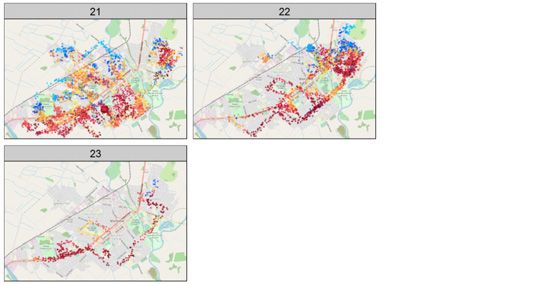
Masterton winter wood-smoke survey, 2018

              optimally - including using appropriately sized wood pieces (i.e., not too big)
              and the correct air flow to avoid a low-heat, smouldering high smoke fire2.

2.3           PM2.5 concentrations from home heating
2.3.1         Daily winter air quality profile measured at air quality monitoring stations
              During winter, average hourly PM2.5 concentrations show a typical pattern of
              low concentrations during the middle of the day, increasing rapidly between
              4pm and 7pm, peaking around 10pm with the duration of the peak persisting
              till after midnight at Masterton East station (Figure 2.3). Concentrations of
              PM2.5 decline overnight and then show a second smaller peak around 9am. This
              diurnal pattern observed in Masterton is very similar to other places in New
              Zealand where wood burners are used for home heating (Trompetter et al.
              2010).

              Figure 2.3: Average winter (June-July 2016 to 2018) PM2.5 (hourly average)
              measured at Masterton air quality monitoring stations (East and West) plotted
              against hour of day (midday to midday)

              Within day and between day variability in PM2.5 concentrations is due to a
              combination of household burning habits and weather patterns.

2.3.2         Wood-burner use
              Intensity of emissions is driven by peoples’ need to heat their homes. Wood-
              burner use follows a general daily pattern, with some differences in use
              reported for the weekend compared to week days. Daily variation in start-up
              times for wood burners and the quantity of wood being burnt is influenced by
              lifestyle and social factors, habits, availability of wood, and temperature

2   http://www.gw.govt.nz/better‐burning/

PAGE 4 OF 30                                                      MASTERTON WOOD SMOKE SURVEY 2018
Masterton winter wood-smoke survey, 2018
(Wilton 2012). In Masterton, most people report lighting their wood-burners
between 17:00 and 19:00 on week nights (Siridha & Wickham 2013). On the
weekend wood burners are used by more people during the middle of the day
and later in the evening compared to weekdays (Figure 2.4).
Wood-burner emissions are not necessarily linearly related to air pollution
levels. There is an approximately four hour time lag between peak wood burner
use (estimated in 2013 by a home heating survey) and peak PM2.5
concentrations measured at both Masterton West and Masterton East air quality
monitoring stations (Figure 2.4).
It is possible that this late peak is due to wood-burner operators re-loading their
fires, then turning down the air supply overnight before the wood has ignited
fully, leading to high smouldering emissions (Innis et al. 2013). There also
appears to be a higher peak in PM2.5 later at night on the weekend that is not
evident in the emissions inventory data (Figure 2.4). A further reason for the
time lag between peak wood burner use and peak night-time concentrations of
PM2.5 measured at the fixed monitoring station is the influences of meteorology
and topography which are discussed in section 2.3 and 2.4 below. A smaller
morning peak in PM2.5 concentrations was also observed and analysis of air
particulate samples shows that is this due to residents re-lighting their fires in
the morning (Ancelet et al. 2012).
Figure 2.4: Typical percentage of wood-burners being used in Masterton by time
of day based on home heating survey (Siridha & Wickham 2013)
2.3.3 Impact of weather patterns and terrain
Weather conditions, as well as emission patterns, strongly influence the day-to-
day variability in measured PM2.5 concentrations. During the winter months
PM2.5 concentrations are lowest during the middle of the day when the air is
PAGE 5 OF 30Masterton winter wood-smoke survey, 2018
typically windier and warmer and therefore pollutants are more readily
dispersed. Furthermore, fewer home fires are in use during the middle of the
day, especially during week days. Typically, temperature and wind speed drop
in the late afternoon and remain low overnight.
On calm and clear nights a radiative temperature inversion can form whereas the
ground cools and heat is lost to space. As air is a poor conductor of heat only the
thin layer of surface air is cooled leaving the air above almost unaffected. This
leads to a layer of warmer air over the top of the cold air underneath, preventing
the cold air from moving upwards and dispersing the wood burner emissions
which have been emitted close to ground level. In this situation even when
people stop using their wood burners, levels of PM2.5 remain elevated for some
time. The temperature inversion can be further strengthened in the Wairarapa
Valley due to cold air drainage from nearby hills leading to cooler air pooling in
lower-lying areas, cooling the ground even further (Griffiths 2011). The
temperature inversion usually breaks up at sunrise when the ground is warmed
and the air becomes more buoyant and moves upwards.
Terrain or landscape also influences the dispersion of emissions as lower lying
areas tend to accumulate air pollution that has drifted down from upslope areas.
Although the Masterton urban area is relatively flat, there is still a gradual
higher north to lower-lying south elevation gradient (Figure 2.5). It has been
suggested that this explains the higher concentrations of fine particles
measured at the lower elevation Masterton East monitoring station compared to
the higher elevation Masterton West station (Ancelet et al. 2012).
Figure 2.5: Digital elevation map (1m resolution) centred on the Masterton urban
area. Darker areas show higher elevation. (Figure courtesy Gareth Palmer, GWRC)
PAGE 6 OF 30 MASTERTON WOOD SMOKE SURVEY 2018Masterton winter wood-smoke survey, 2018
3. Objectives
To test the ability of mobile monitoring, using a SmokeTrak instrument, to
identify spatial patterns in wood-smoke concentration.
To assess how well the fixed monitoring stations represent wood-smoke
levels in un-monitored areas.
To identify suburbs or parts of suburbs with elevated wood-smoke
concentrations that may warrant further investigation.
PAGE 7 OF 30Masterton winter wood-smoke survey, 2018
4. Methodology
4.1 Car-based monitoring
Mobile air quality monitoring was conducted across Masterton using a
“SmokeTrak” instrument mounted inside a car. The survey was undertaken on a
number of evenings during June and early July 2018. The SmokeTrak instrument
was developed by Kenelec Scientific Pty Ltd (Australia) for the Firewood
Association of Australia Inc. and is based on the Travel BLANkET3 system first
developed by the Tasmanian Environmental Protection Authority for smoke
survey measurements (Innis et al. 2013). This technology has been used in the
Tasmanian domestic smoke management programme “Burn brighter this
winter”, a community education project which has been running since 2012.
The SmokeTrak unit, hired from Kenelec Scientific Pty Ltd (Australia), is
specifically designed for mobile monitoring of wood-smoke. The instrument
consists of a TSI DustTrak Aerosol Monitor (model 8533) with an in-line
PM2.5 filter housed in a travel case together with a GPS sensor, a modem and a
tablet for displaying measured PM2.5 concentrations. The unit was placed on
the passenger side inside the vehicle with the sample inlet attached to the
outside the front window of the car. The unit was powered using the vehicles
12-volt power outlet (Figure 4.1). When switched on, a pump in the
SmokeTrak sampled air from outside the car at a rate of 3 litres per minute
through the inlet tube. The sampled air was passed through the auto zero
module which corrected for zero drift in the DustTrak at 1-hour intervals.
Particle concentration readings (µg/m3) were sent continuously to the Agent
G2 data logger which transmitted the readings to the Pervasive Telemetry
website every 5 seconds together with the current GPS co-ordinates. The
SmokeTrak data was able to be viewed in real-time on the Pervasive Telemetry
website using the tablet provided. The vehicle containing the SmokeTrak was
driven at approximately 30 km/hour meaning a PM2.5 measurement was
captured at roughly 8 m intervals along the route. Each measurement was
timestamped and geo-referenced by a GPS connected to the SmokeTrak.
Figure 4.1: SmokeTrak measuring system set up in monitoring vehicle
3 Base-Line Air Network of EPA Tasmania
PAGE 8 OF 30 MASTERTON WOOD SMOKE SURVEY 2018Masterton winter wood-smoke survey, 2018
4.2 Sampling route
The driving route was planned to cover as much of Masterton’s urban area as
possible within a three-hour period. Approximately 70 km of a driving route
was able to be monitored at a speed of 30km/hr over a three hour period.
Sampling was undertaken between 17:00 and 23:00 to capture the range of
wood-smoke concentrations, from initial start-up through to later in the
evening. It was originally planned to monitor on 12 nights that were clear and
calm to minimise the night-to-night difference in wood-smoke levels due to
meteorological effects. Due to the above average June rainfall4 there were
fewer dry and low wind speed nights only eight nights were both suitable for
monitoring and had personnel available to carry out the monitoring.
4.3 Data processing and GIS analysis
(i) The SmokeTrak 5-second measurements were downloaded as a csv
file from the Pervasive Telemetry website after each sample run.
These files were merged and calibration data points, when the
instrument was in auto-zero mode, were removed.
(ii) PM2.5 and meteorological measurements (10 minute averages) from
the fixed stations (Masterton East and Masterton West) were then
matched to the nearest minute of the timestamped SmokeTrak
measurement.
(iii) On two separate evenings, the SmokeTrak unit was parked close to the
Masterton East monitoring station for a period of several hours so that
the SmokeTrak measurements could be compared to measurements
made by the fixed reference monitor (Beta Attenuation Monitor,
model 5014i) at Masterton East. The 10-minute average SmokeTrak
measurements were approximately three times higher than those
measured by the reference monitor. This difference arose as the
SmokeTrak as supplied was calibrated with latex spheres (A1-
ultrafine dust) and needed to be re-calibrated to report appropriate
mass concentrations for smoke aerosols (John Innis pers. comm.
22/10/2018). To account for the difference in measurement between
the fixed reference monitor and the SmokeTrak, the mobile 5-second
averages were adjusted downwards based on the collocated
measurements as described in Appendix A1.
(iv) The SmokeTrak data were converted to a spatial data points file based
on the latitude and longitude coordinates captured by the GPS. The
spatial data points were then clipped to the boundary of the Masterton
urban area so that measurements outside the urban area were removed.
(v) To simplify visual representation of the data, the SmokeTrak
measurements were aggregated over a 200m x 200m grid which was
superimposed on an OpenStreetMap of the Masterton urban area.
(vi) A single high emitting chimney can produce very high levels of PM2.5
which can be measured if the SmokeTrak passes through the plume.
4 http://www.gw.govt.nz/assets/2018-uploads/Climate-and-Water-Resource-SummaryColdSeason-2018.pdf
PAGE 9 OF 30Masterton winter wood-smoke survey, 2018
To remove the influence of extreme SmokeTrak values due to
transient high chimney smoke events, the SmokeTrak dataset was
trimmed to remove the top 5% of measurements. This trimmed dataset
is closer to the distribution of the Masterton East PM2.5 reference
monitor measurements (Appendix A1).
(vii) Data analysis, plots, spatial aggregation and mapping were carried out
using R (R Core Team 2017) using the following packages:
tmap/tmaptools (Tennekes 2018)
rgdal (Bivand et al. 2018)
rgeos (Bivard & Rundel 2017)
dplyr (Wickham et al. 2017)
sp (Pebesma & Bivand 2005; Bivand & Pebesma 2013)
RColorBrewer (Neuwirth 2014)
ggplot(Wickham 2009)
openair(Carslaw & Ropkins 2012)
The Masterton base map was downloaded from OpenStreetMap5.
5 https://www.openstreetmap.org/#map=10/-41.1264/175.4723
PAGE 10 OF 30 MASTERTON WOOD SMOKE SURVEY 2018Masterton winter wood-smoke survey, 2018
5. Results and discussion
5.1 Summary of SmokeTrak measurements
We collected approximately 21,000 5-second PM2.5 measurements using the
SmokeTrak over eight separate evenings and two mornings (Table 5.1). The
daily average wind speed, minimum daily 1-hour temperature and 24 hour
average PM2.5 measured at Masterton East are shown in Figure 5.1. The
sampled evenings covered a range of meteorological conditions (Table 5.2).
Table 5.1: Summary of SmokeTrak-adjusted and Masterton East air quality
monitoring station PM2.5 (µg/m3) concentrations (SD in brackets)
Date Day Start End SmokeTrak- Number Masterton Masterton Masterton
of adjusted of data East PM2.5 East PM2.5 East PM2.5
week PM2.5 points (averaged (6hr- (24-hour
over same average average
period as 17:00- midnight
SmokeTrak) 23:00) to
midnight)
14/6/2018 Thu 17:04:30 21:14:40 61.2 (30.7) 2426 41.6 (7.5) 42.7 19.7
15/6/2018 Fri 08:32:00 09:21:45 43.5 (28.5) 517 20.2 (15.9) NA 18.7
20/6/2018 Wed 19:11:50 22:15:15 41.6 (49.2) 1321 37.5 (11.0) 39.2 16.3
21/6/2018 Thu 08:32:30 09:15:50 65.6 (24.3) 460 43.5 (11.5) NA 39.1
23/6/2018 Sat 19:05:10 22:55:25 116.3 (59.7) 2514 146.2 (42.3) 130.6 49.9
27/6/2018 Wed 17:16:00 22:19:35 34.7 (26.3) 3010 33.4 (21.3) 36.8 21.6
28/6/2018 Thu 18:50:40 22:14:25 68.3 (45.7) 2319 58.5 (32.7) 42.7 24.6
30/6/2018 Sat 17:26:40 23:39:40 121.8 (68.8) 3276* 134.8 (57.5) 135.4 60.7
3/7/2018 Tue 17:12:30 22:13:20 65.5 (56.1) 2855 65.7 (45.8) 65.7 23.7
4/7/2018 Wed 19:08:20 23:05:45 98.5 (57.1) 2594 94.3 (22.3) 85.6 39.1
*includes mobile monitoring in Carterton from 17:42 to 20:13
Table 5.2: Summary of weather conditions for mobile sampling evenings (17:00 to
23:00) as measured at the Masterton West air quality monitoring station (10m)
Date Mean Mean Tmin 10- Tmax Wind Rainfall
wind temp 1-hr min (oC) 10-min direction accumulation
speed 1- (oC) (oC) (mm)
hr (m/s)
14/6/2018 0.6 8.7 5.9 10.8 NW 0
20/6/2018 1.1 4.7 4.0 5.6 SW 0.4
23/6/2018 0.8 6.1 4.1 9.1 NE 0
27/6/2018 1.3 6.5 3.4 8.8 SW 0
28/6/2018 1.1 4.5 1.5 8.3 NW 0
30/6/2018 0.9 3.2 0.7 7.9 N 0
3/7/2018 0.9 3.6 0.2 6.7 SW 0
4/7/2018 1.0 3.2 0.0 8.5 W 0
PAGE 11 OF 30Masterton winter wood-smoke survey, 2018
Figure 5.1: Daily average wind speed and daily 1-hour temperature minima
recorded at Masterton West (10m) during June and July 2018. The dashed line
shows the five year average (2012-2017) for wind speed and minimum
temperature. The black dots show the mobile monitoring dates.
The altitude measurements of the mobile GPS were not as accurate as the
latitude longitude coordinates. Nevertheless, the GPS measurements (Appendix
A2) showed the same general pattern as the 1-m digital elevation map of the
Masterton urban area and so were adequate for data interpretation (Figure 2.5).
5.2 ‘Smokiness’ of the sampling nights
Figure 5.2 shows the distribution of all PM2.5 6-hour averages (17:00 to 23:00)
recorded at the Masterton East monitoring for all evenings during June and
July for the past five years. In this box plot the boxes range from the 25th to
75th percentile. The range between these percentiles is known as the
interquartile range (IQR). The horizontal lines through the boxes represent the
median. The whiskers start from the edge of the box (ie, the 25th and 75th
percentiles) and extend to the furthest data point that is within 1.5 times of the
IQR. Any data points that are past the ends of the whiskers are considered
outliers (or extreme values) and are displayed with dots. The 6-hour averages
recorded at the Masterton East station during the mobile sampling nights are
annotated with labelled dates.
Four of the sample evenings (14/6, 20/6, 27/6 and 28/6) had moderate PM2.5
levels (ie, 10-50 µg/m3), two evenings (3/7 and 4/7) had high PM2.5 levels (ie,
50-100 µg/m3) and two evenings (23/6 and 30/6) had very high PM2.5 levels (ie,
PAGE 12 OF 30 MASTERTON WOOD SMOKE SURVEY 2018Masterton winter wood-smoke survey, 2018
above 100 µg/m3). No low pollution nights were sampled and so the SmokeTrak
monitoring was skewed towards higher levels of wood smoke than an average
winter’s evening. Figure 5.3 shows the relative concentrations of PM2.5 for each
evening in June and July 2018 and the wind direction and wind speed.
Figure 5.2: Distribution of 6-hour average PM2.5 (17:00 to 23:00) measured at the
Masterton East air quality monitoring station for June-July from 2014 to 2018. Labels
show the location in the distribution of evening PM2.5 measured at the Masterton East
station for the dates of SmokeTrak mobile monitoring. The horizontal lines show the
median PM2.5 concentration for the evening period for each year.
Figure 5.3: Calendar plot (Saturday to Friday each week) showing daily average
PM2.5 (µg/m3) measured at the Masterton East air quality monitoring station. The
arrows show wind direction scaled to wind speed (ie, longer the arrow the higher
the wind speed) for the period 17:00 to 23:00 for June and July 2018 with dates of
sample nights shown.
PAGE 13 OF 30Masterton winter wood-smoke survey, 2018
5.3 Time variation in wood smoke measurements
The time variation in SmokeTrak PM2.5 measurements (10-minute averages),
averaged over all evening sample runs, follow roughly the same pattern as
PM2.5 measured at the Masterton East air quality monitoring station (during the
sample evenings) until 22:00 (Figure 5.4). After 22:00 the SmokeTrak
measured higher concentrations relative to Masterton East. This may be a
consequence of sampling having been biased towards lower-lying areas of
town during 22:00 and midnight as shown in Appendix A4 where all
SmokeTrak measurements are mapped by hour of the evening.
Figure 5.4: Ensemble of PM2.5 (10-minute averages µg/m3) aggregated over all
monitoring evenings measured by SmokeTrak-adjusted (blue) and at the
Masterton East air quality monitoring station (red)
5.4 Wood smoke maps
5.4.1 SmokeTrak 5-second averages
Figure 5.5 shows the individual 5-second PM2.5 averages collected by the
SmokeTrak over the eight evenings sampled in Masterton. There was large
variation in fine-scale wood-smoke measurements. Some streets had both high
and low concentrations representing monitoring occurring on different nights
or different times of the evening. The individual SmokeTrak data points (with
top 5% removed) for all monitoring runs are shown by the evening sampled in
Appendix A3 and by hour of day in Appendix A4. Figure 5.5 shows that higher
concentrations of PM2.5 were mainly found to the east, south and southwest
with the lowest concentrations outside of the main urban area and at higher
elevations in the suburb of Lansdowne.
PAGE 14 OF 30 MASTERTON WOOD SMOKE SURVEY 2018Masterton winter wood-smoke survey, 2018
Only two short mobile monitoring runs were undertaken in the morning period
between 08:30 and 09:15 (Figure 5.6). Whist there are not enough data points
to be definitive, there appears to be a similar pattern to evening concentrations,
with lower-lying areas being worst affected.
At very local spatial scales, tens of metres, a single excessively smoke emitting
chimney can produce very high levels of PM2.5. Mobile measurements may
capture very high readings if the monitor passes through the plume. Likewise
the high readings may not be captured if the mobile monitor is upwind of this
high concentration plume. The 95th percentile of SmokeTrak-adjusted
measurements are shown in Figure 5.7. These are the top 5% of measurements
and may represent local ‘hot spots’ due to high emitting chimneys. These
clusters of extremely high short-term PM2.5 levels were mainly found in parts
of the Solway North, Solway South, Masterton East and lower lying areas in
the Lansdowne suburb. Most of these top 5% of measurements were made on
the high to very high pollution nights between 19:00 and midnight.
5.4.2 SmokeTrak grid cell averages
Figure 5.8 shows the SmokeTrak-adjusted PM2.5 measurements averaged over
a 200m grid - where each grid area was visited on at least five separate
monitoring nights (sample runs). This is a reduced dataset because some cells
received fewer than five visits with the SmokeTrak. This map shows that some
areas of Masterton appear to be more impacted by wood smoke than others and
lower lying areas show a consistent pattern of high wood-smoke levels. These
low-lying areas were disproportionally sampled at 22:00 and midnight which
means that the high concentrations will be reflecting the time variation as well
as spatial variation.
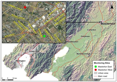
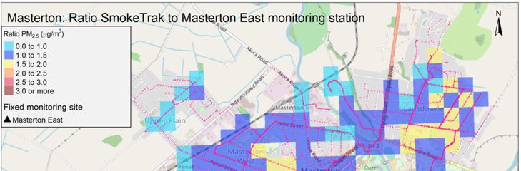
5.4.3 SmokeTrak grid cell ratio to fixed monitoring station
Figure 5.9 was produced by taking the ratio of each SmokeTrak-adjusted PM2.5
mobile measurement to what was measured at the Masterton East station over
the matching time period and then averaging all the ratios over a 200m grid.
Each grid cell therefore represents an average of all the ratios, where each grid
area was visited on at least five separate monitoring nights (sample runs).
This is a reduced dataset because some cells received fewer than five passes
with the SmokeTrak. The blue areas were on average lower or similar to what
was measured at the Masterton East air quality monitoring station. The yellow
to orange areas were, on average, higher than what was measured at Masterton
East air quality monitoring station and the dark brown areas were very elevated
compared to the Masterton East air quality monitoring station. This suggests
that some areas such as parts of Solway North may experience much higher
wood-smoke at times than measured at the air quality monitoring station.
PAGE 15 OF 30Masterton winter wood-smoke survey, 2018
Figure 5.5: SmokeTrak-adjusted PM2.5 µg/m3 (5-second averages) measured in Masterton over eight evenings in June and July 2018 (top 5%
of measurements removed), n=17,839. Points are ‘jittered’ to minimise overlapping data points
PAGE 16 OF 30Masterton winter wood-smoke survey, 2018
Figure 5.6: SmokeTrak-adjusted PM2.5 µg/m3 (5-second averages) measured in Masterton over two sampled mornings in June 2018, n=971.
Points are ‘jittered’ to minimise overlapping data points
PAGE 17 OF 30Masterton winter wood-smoke survey, 2018
Figure 5.7: 95th percentile SmokeTrak-adjusted PM2.5 µg/m3 (5-second averages) collected during the eight evening sample runs through
June and July 2018 (top 5% of measurements), n=936
PAGE 18 OF 30Masterton winter wood-smoke survey, 2018
Figure 5.8: SmokeTrak-adjusted PM2.5 µg/m3 (5-second averages) (trimmed dataset with top 5% of measurements removed) aggregated to a
200m x 200m grid, where each grid cell represents the average of measurements from at least five separate monitoring evenings. Mobile
monitoring data points shown as pink-coloured dots.
PAGE 19 OF 30Masterton winter wood-smoke survey, 2018
Figure 5.9: Ratio of mobile SmokeTrak-adjusted PM2.5 (µg/m3) measurements (top 5% removed) to PM2.5 recorded at the same time at the
Masterton East air quality monitoring station (black triangle). All measurements averaged to a 200m x 200m grid, where each grid cell
represents the average of ratios of measurements from at least five separate monitoring evenings. Mobile monitoring data points shown as
pink-coloured dots.
PAGE 20 OF 30Masterton winter wood-smoke survey, 2018
5.4.4 Limitations
As these maps were generated from a relatively small number of sample
evenings they may represent a ‘snapshot’ of air quality at a particular location
and not necessarily reflect overall winter air quality patterns. The mobile
monitoring path was restricted to roads and therefore doesn’t cover all areas
impacted by wood smoke. There is a time lag of approximately 10 seconds
between the intake of smoke and its detection by the SmokeTrak which is not
compensated for by the instrument’s software. This means that the SmokeTrak
measurement is spatially located to where the car was 10 seconds earlier. In
most cases this effect is small, but needs to be considered, particularly if the
SmokeTrak was to be used to identify individual chimneys – which was not a
monitoring objective of this study.
PAGE 21 OF 30Masterton winter wood-smoke survey, 2018
6. Conclusion
The car-based monitoring method using the SmokeTrak instrument provided
useful information on the spatial variation of wood-smoke across the Masterton
urban airshed. The method shows that with sufficient sampling runs persistent
‘hot spots’ of high wood-smoke can be identified.
On high pollution nights, peak concentrations occurred later in the evening
(after 10 pm) in the low-lying areas of Masterton East, Lansdowne and Solway
South. Concentrations of PM2.5 in these areas were likely higher than those
measured at the Masterton East monitoring station as cold air slowly moved
from higher to lower altitude areas, leading to an accumulation of wood-smoke
in the lower-lying areas.
Clusters of very high transient PM2.5 measurements were identified in some
parts of the suburbs of Solway, Kuripuni, Masterton East and Lansdowne.
More on the ground observations are needed to confirm whether these high
PM2.5 observations were due to consistently high emitting chimneys that could
be targeted for some form of assistance to reduce emissions.
Mobile-monitoring is labour-intensive and it is recommended that a further
complementary study be carried out using a distributed network of low-cost
sensors that could set up for a one to two month campaign to include the
potential hot spot areas identified in this study.
PAGE 22 OF 30Masterton winter wood-smoke survey, 2018
Acknowledgements
This project would not have been possible without the contributions of Matt Noora,
Agnes Piatek-Bednarek and Alex Carter (MDC) who assisted with the mobile
monitoring. John Innis (Tasmanian Environmental Protection Agency provided valuable
technical advice on survey design and data analysis and mapping. Roger Uys (GWRC)
helped with technical aspects of GIS and GPS measurements and provided helpful
comments on the report.
PAGE 23 OF 30Masterton winter wood-smoke survey, 2018
References
Ancelet T, Davy PK, Mitchell T, Trompetter WJ, Markwitz A, and Weatherburn DC.
2012. Identification of Particulate Matter Sources on an Hourly Time-Scale in a Wood
Burning Community. Environmental Science & Technology, 46(9), 4767–4774.
https://doi.org/10.1021/es203937y
Ancelet T, Davy PK, Trompetter WJ, Markwitz A, and Weatherburn DC. 2013.
Carbonaceous aerosols in a wood burning community in rural New Zealand.
Atmospheric Pollution Research, 4(3), 245–249.
https://doi.org/10.5094/APR.2013.026
Bivand R, Keitt T and Rowlingson B. 2018. rgdal: Bindings for the 'Geospatial' Data
Abstraction Library. R package version 1.3-4. https://CRAN.R-
project.org/package=rgdal
Bivand R and Rundel C. 2017. rgeos: Interface to Geometry Engine - Open Source
('GEOS'). R package version 0.3-26. https://CRAN.R-project.org/package=rgeos
Bivand RS, Pebesma E and Gomez-Rubio V. 2013. Applied spatial data analysis with
R, Second edition. Springer, New York. http://www.asdar-book.org/
Carslaw DC and Ropkins K. 2012. openair --- an R package for air quality data analysis.
Environmental Modelling & Software. Volume 27-28, 52-61
Chapell PR. 2014. The climate and weather of Wellington. 2nd edition. NIWA Science
and Technology Series number 65.
Innis J, Bell A, Cox E, Cunningham A, Hyde B and Smeal A. 2013. Car-based surveys
of winter smoke concentrations in some Tasmanian towns, 2010-2012. Proceedings of
the 21st CASANZ conference: Sydney, 7-11 September 2013. ISBN 9780987455321.
McGreevy A, Barnes G. 2016. Domestic wood smoke reduction in the urban
environment. Prepared for the Firewood Association of Australia Inc. Victoria,
Australia.
Mitchell T. 2016. Carterton winter air quality: 2010 to 2016. Greater Wellington
Regional Council, Publication No. GW/ESCI-T-16/96, Wellington.
http://www.gw.govt.nz/assets/council‐publications/Carterton‐winter‐air‐quality‐2010‐
to‐2016.pdf
Neuwirth E. 2014. RColorBrewer: ColorBrewer Palettes. R package version 1.1-2.
https://CRAN.R-project.org/package=RColorBrewer
Pebesma EJ and Bivand RS. 2005. Classes and methods for spatial data in R. R News 5
(2), https://cran.r-project.org/doc/Rnews/.
R Core Team. 2017. R: A language and environment for statistical computing. R
Foundation for Statistical Computing, Vienna, Austria. URL https://www.R-
project.org/.
PAGE 24 OF 30Masterton winter wood-smoke survey, 2018
Sridhar S, and Wickham L. 2013. Masterton and Carterton domestic fire emissions
inventory 2013. Prepared by Emission Impossible Ltd for Greater Wellington Regional
Council, August 2013.
Tennekes M. 2018. “tmap: Thematic Maps in R.” _Journal of Statistical Software_,
*84*(6), pp. 1-39. doi: 10.18637/jss.v084.i06
(URL:http://doi.org/10.18637/jss.v084.i06)
Todd J J. 2003. Wood-smoke handbook: Woodheaters, firewood and operator practice.
For the Natural Heritage Trust, commissioned by Environment Australia and NSW
Environment Protection Agency.
Trompetter WJ, Davy PK and Markwitz A. 2010. Influence of environmental conditions
on carbonaceous particle concentrations within New Zealand. Special Issue for the 9th
International Conference on Carbonaceous Particles in the Atmosphere, 41(1), 134–142.
https://doi.org/10.1016/j.jaerosci.2009.11.003
Trompetter WJ, Grange SK, Davy PK, Ancelet T and Markwitz A. 2010. Black carbon
transect profiles during the 2010 winter sampling campaign in Masterton, New Zealand.
CASANZ 2011 Conference, Auckland. 31 July to 2 August. Paper 216.
Wickham H. 2009. ggplot2: Elegant Graphics for Data Analysis. Springer-Verlag New
York.
Wickham H, Francois R, Henry L and Müller K. 2017. dplyr: A Grammar of Data
Manipulation. R package version 0.7.2. https://CRAN.R-project.org/package=dplyr
Wilton E. 2012. Review particulate emissions from woodburners in New Zealand.
Prepared for NIWA. Environet Ltd, Christchurch.
World Health Organization. 2006. WHO air quality guidelines for particulate matter,
ozone, nitrogen dioxide and sulfur dioxide – global update 2005. Retrieved from
http://www.who.int/phe/health_topics/outdoorair_aqg/en/
PAGE 25 OF 30Masterton winter wood-smoke survey, 2018 Appendix A1: Co-location relationship – SmokeTrak and air quality monitoring station PM2.5 measurements The SmokeTrak measures PM2.5 using an optical method (light-scattering photometer) and the instruments at the fixed monitoring stations (5014i Thermo Scientific) use beta attenuation. These two methods produce different results. The instruments at the fixed station are reference methods that are used for assessing compliance with the national environmental standards. In order to compare SmokeTrak measurements to the fixed station measurements, the vehicle containing the SmokeTrak was parked close the Masterton East station on two evenings for several hours to obtain co-located measurements. The 10-minute averages from both instruments were correlated with the SmokeTrak consistently measuring higher concentrations than the instrument at the monitoring station (Figure A1.1). Based on this relationship the 5-second SmokeTrak measurements were adjusted downwards so they can be compared to those at the fixed station. The distributions of the measurements made at the stations and of the adjusted SmokeTrak 5-second averages are shown in Figure A1.2). Figure A1.1: Correlation between SmokeTrak and the Masterton East air quality monitoring station instrument (5014i) 10 minute averages PAGE 26 OF 30
Masterton winter wood-smoke survey, 2018

Figure A1.2: Left: Boxplot SmokeTrak-adjusted PM2.5 (5-second averages) and fixed station
PM2.5 (10-minute averages) over all monitoring evenings in Masterton. The red line is the
95th percentile of SmokeTrak-adjusted measurements, n=18,775. Right: Boxplot
SmokeTrak-adjusted 5-second averages and air quality monitoring station 10-minute for
all measurements below the 95th percentile (ie, top 5% removed), n=17,839.

                                                                                               PAGE 27 OF 30
Masterton winter wood-smoke survey, 2018 Appendix A2: GPS-recorded measurements of altitude along monitoring route Figure A2.1: Altitude (m a.s.l.) measurements recorded by GPS during the mobile measurements. Dark blue shows the lowest lying areas. PAGE 28 OF 30
Masterton winter wood-smoke survey, 2018
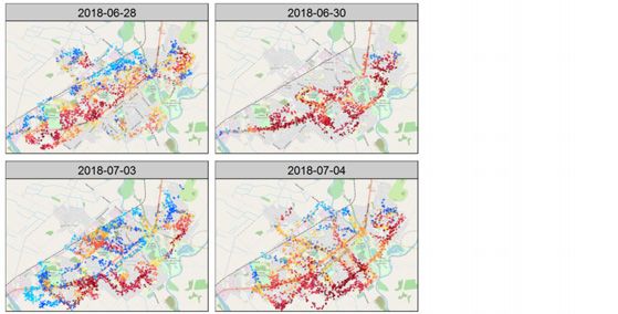
Appendix A3: Masterton SmokeTrak measurements by sample
date
Figure A3.1: Trimmed SmokeTrak-adjusted PM2.5 µg/m3 (5-second averages) measured in
Masterton over all hours between 17:00 and 23:39 (top 5% of measurements removed) by
sample date
PAGE 29 OF 30Masterton winter wood-smoke survey, 2018 Appendix A4: Masterton SmokeTrak measurements by hour Figure A4.1: Trimmed SmokeTrak-adjusted PM2.5 µg/m3 (5-second averages) measured in Masterton during all sampled evenings (top 5% of measurements removed) shown by hour of day. Note the 23:00 hour subplot is based mostly on observations during the evening of 30/06/2018 when sampling continued until 23:39. PAGE 30 OF 30
You can also read