Intermittency in phytoplankton bloom triggered by modulations in vertical stability - Nature
←
→
Page content transcription
If your browser does not render page correctly, please read the page content below
www.nature.com/scientificreports
OPEN Intermittency in phytoplankton
bloom triggered by modulations
in vertical stability
Madhavan Girijakumari Keerthi*, Marina Lévy & Olivier Aumont
Seasonal surface chlorophyll (SChl) blooms are very chaotic in nature, but traditional bloom
paradigms have climbed out of these subseasonal variations. Here we highlight the leading order
role of wind bursts, by conjoining two decades of satellite SChl with atmospheric reanalysis in the
Northwestern Mediterranean Sea. We demonstrate that weekly SChl fluctuations are in phase with
weekly changes in wind stress and net heat flux during the intial state of the bloom in winter and
early spring, thus expanding the convection shutdown hypothesis of bloom onset to subseasonal
timescales. We postulate that the mechanism reflected by this link is intermittency in vertical stability
due to short-term episodes of calm weather in winter or to stormy conditions in early spring, leading
to short-term variations in light exposure or to events of vertical dilution. This strong intermittency in
phytoplankton bloom may probably have important consequences on carbon export and trophic web
structure and should not be overlooked.
A striking characteristic of phytoplankton blooms are the fluctuating patterns in sea-surface Chlorophyll (SChl, a
proxy for phytoplankton biomass) that punctuate the transition from low abundance in winter to biomass accu-
mulation in s pring1–10. The chaotic nature and varying intensity of these subseasonal events make each seasonal
cycle unique. In some years, the temporal evolution of SChl deviates from the traditional pattern characterized
by a single seasonal peak and exhibits a succession of several p eaks8. These subseasonal events make an important
contribution to bloom variability8 and are therefore an important factor for the development of the upper trophic
levels of the food web11 as well as for the efficiency of the biological carbon pump12.
Traditional bloom onset paradigms have climbed out of these subseasonal variations by focusing on the
strongest, or latest, peak. They relate the period of rapid growth of SChl between winter and spring to the
change in vertical stability, and to the increased light exposure of the phytoplankton population associated with
it. Under these models, a sustained bloom cannot start before a seasonal tipping point is met, such as a critical
depth or critical mixing intensity10,13–20. This view is in conflict with the strong chaotic intermittency seen in
SChl time series. Incidentally, evidences of intermittent near-surface phytoplankton accumulation during spells
of calm weather in winter, with biomass being mixed down in the next storm, leading to a decrease in SChl until
weather conditions improve again, were present in the data sets used to test spring bloom models13,14 but have
been overlooked.
Here we explore the links between the surface bloom and vertical stability at intraseasonal timescales, using
two decades of satellite SChl data and atmospheric reanalysis in the Northwestern Mediterranean Sea. Our
focus on this region is motivated by a previous study that highlighted the strong intensity of subseasonal SChl
fluctuations there8. At the seasonal time scale, Ferrari et al.13 showed that surface blooms in the North Atlantic
were triggered by a change from cooling to heating in Net Heat Flux (NHF) at the end of winter, with a similar
dataset. They argued that this change resulted in a rapid shutdown of vertical convection. The physical basis
came from a preliminary numerical study which demonstrated that the reduction in air-sea fluxes at the end of
winter could be used as an indicator of reduced turbulent m ixing10. Our intention is to generalize this concept
to all time scales from seasonal to subseasonal. Intermittency in turbulent mixing being primarily driven by
intermittency in atmospheric forcing, we want to test whether subseasonal changes in SChl can be explained by
subseasonal changes in atmospheric conditions.
The seasonal phenology of SChl in the Northwestern Mediterranean Sea is well d ocumented21. As in the
North Atlantic, it has been traditionally related to changes in the mixed-layer depth (MLD)22,23, with the SChl
bloom starting as soon as the water column is more stable, and a time lag of about 1 month between the time of
maximum MLD in winter and maximum SChl in spring. As a first step, we verified that the convection shutdown
Sorbonne Université (CNRS/IRD/MNHN), LOCEAN-IPSL, Paris, France. *email: keerthi.madhavan‑girijakumari@
locean.ipsl.fr
Scientific Reports | (2021) 11:1285 | https://doi.org/10.1038/s41598-020-80331-z 1
Vol.:(0123456789)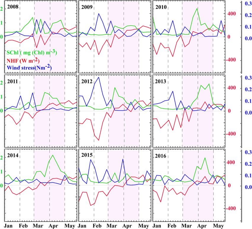
www.nature.com/scientificreports/
hypothesis of seasonal bloom i nitiation13 applied to this region. This hypothesis is easier to test and more precise
than the critical depth hypothesis14 because the surface mixed-layer is not always associated with strong rates
of turbulent m ixing1,24. As a second step, we investigated the hypothesis that subseasonal modulations in verti-
cal stability triggered by wind bursts (and reflected by temporal variations in NHF) explain subseasonal SChl
variations during the initial states of the bloom in the Northwestern Mediterranean Sea. The paper ends with a
discussion on uncertainties and wider implications of these results.
Results
Our focus is on the winter (January–February) to spring (March–April) period, which covers the entire SChl
bloom from its onset to its decay. This is also when storms are the most frequent and subseasonal variations in
SChl are intense8. We first describe the main seasonal changes in SChl between winter and spring and relate
them to changes in NHF. We then extend the analysis to subseasonal fluctuations.
The Northwestern Mediterranean Sea is one of the few regions in the world’s ocean where deep convection
occurs25. During winter, a deep-mixed patch of dense, nutrient rich water is formed during intense mixing epi-
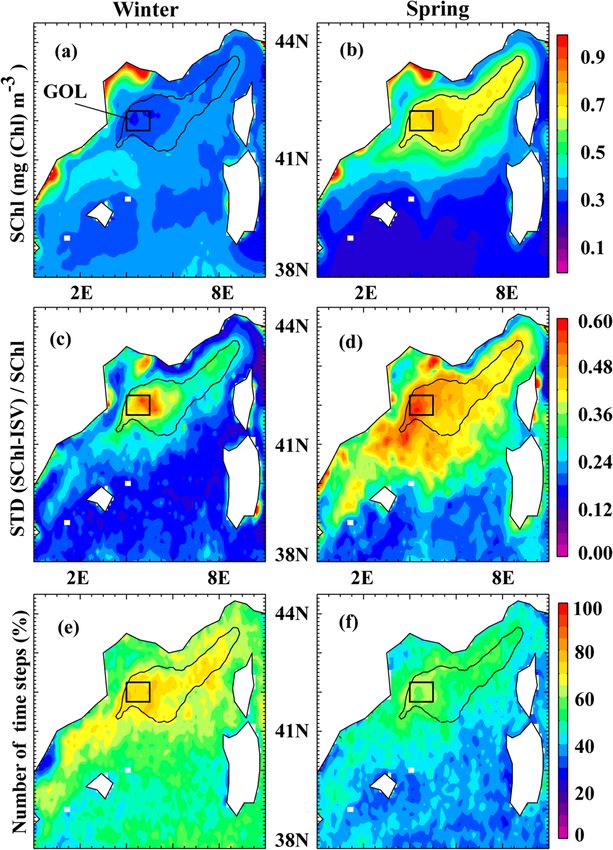
sodes and appears as a blue zone devoid of SChl in ocean color i mages26 (Fig. 1a). The air-sea heat budget shows
a mean seasonal trend from strong buoyancy losses in winter to strong gains in spring, associated with warming.
This trend drives seasonal stratification. Consequently, in spring, the pattern in SChl is the reverse figure of the
winter pattern (Fig. 1b): the largest spring SChl values mirror the lowest SChl winter values, which delineate the
convective area and the corresponding largest winter nutrient inputs27.
SChl time series between winter and spring in the core of the bloom region between 2008 and 2016 provide
a few examples of the annually repeating SChl spring bloom (GOL Box, Fig. 2). The complete time series from
1998 to 2017 is provided in Supplementary Fig. S1. SChl are generally lowest in February, increase sharply around
mid-March and decrease in April. There are numerous exceptions to this general rule, and these will be discussed
later. For now, we examine whether the main seasonal increase in SChl occurs concurrently with the change of
sign in NHF, in support of the convection shut down hypothesis13.
A general feature is that the NHF turns positive in mid-March and remains positive thereafter (Fig. 2 and
Supplementary Fig. S1). This change of sign consistently coincides with a sharp increase in SChl. This is more
quantitatively seen in Fig. 3a which shows the value of the SChl net growth rate at the time at which NHF turns
and remains positive (t = 0) and at three consecutives 8-day periods before and after t = 0 (t = − 24d, − 16d, − 8d,
8d, 16d, 24d), over the entire time series (1998–2017) and for the entire bloom region. Averaged over all events,
the net growth rate is ~ 0.1 day−1 at t = 0 but it is close to zero otherwise. Indeed, the net growth rate is always
strictly positive (between 0 and 0.2 day−1) for each individual event at t = 0, whereas before and after t = 0, net
growth rates are more equally distributed between positive and negative values. This result expands the results
of Ferrari et al.13 to the Northwestern Mediterranean Sea. Incidentally, Fig. 3a also reveals large values of the
standard deviation of the net growth rates, indicating large values of the net growth rate at times before and after
t = 0, which we will examine thereafter.
Now we examine the subseasonal events that punctuate the mean seasonal evolution. These subseasonal
variations have large intensity both during winter and during spring, although the spatial extent of the region
where their intensity is large is more limited in winter than in spring (Fig. 1c,d). Subseasonal variations induce
a large variety of typologies of the SChl evolution (Fig. 2 and Supplementary Fig. S1). The seasonal evolution
of SChl seldom shows as a single period of rapid SChl accumulation in spring. There can be early periods of
accumulation in February (2008, 2011), a series of two to three well separated periods of accumulation of similar
magnitude during spring (2008, 2015), a main period of accumulation followed by (2010, 2012) or preceded by
(2011, 2014) smaller peaks, or double-headed peaks (2009, 2013, 2016).
In order to explore the link between short term episodes of calm weather in winter or intensified mixing in
spring with intraseasonal SChl fluctuations, we examined the relationship between the time derivative of the NHF
and the net SChl growth rate, for each 8-day time step in winter and spring. The underlying assumption is that
periods of reduced mixing during winter should correspond to less negative NHF (and lower wind stress), while
periods of intensified mixing in spring correspond to lower NHF (and stronger wind stress). The comparison
of NHF and wind stress (WS) time series (Fig. 2 and Supplementary Fig. S1) clearly reveals that subseasonal
variations of NHF mirror those of the WS. One recurrent feature is that the seasonal increase in NHF is inter-
rupted by storms that last for about one time step (i.e. less than a week). These storms occur several times every
year and some were particularly strong such as in Feb 2012. Some winters were rather mild (2008, 2014, 2016),
some springs particularly stormy (2008, 2009, 2015). Over the bloom region, and from 1998 to 2017, the relative
proportion of 8-day bins during which a positive variation in NHF (or a negative variation in WS) was associated
with a positive variation in SChl or vice-versa was around 70% in winter and 55% in spring (Fig. 1e,f).
We examined separately three types of situations which we distinguished based on the sign of the NHF during
two consecutive 8-day time steps (Fig. 3b–d): (1) the unstable winter situation, when active turbulent mixing
takes place (NHF are negative during the first 8-day time step and remain negative during the following time
step), (2) the transition phase, when convection shuts down (NHF are negative during the first time step and posi-
tive during the second time step) or when convection resumes (NHF are positive during the first time step and
switch to negative during the second time step) and (3) the stable spring situation, when mixing is weak (NHF
are initially positive and remain positive). There were several years (for instance 2008, 2010 and 2013) where
the NHF oscillated between positive and negative values before transitioning to positive. During such years, in
Fig. 3a, we only accounted for the last zero-crossing to test the convection shutdown hypothesis, as in Ferrari
et al.13. In Fig. 3b, which shows the net growth rate against the time derivative of the NHF during the transition
period, we accounted for all zero-crossing events. This enabled us to extend the initial concept of the convection
shutdown hypothesis to weekly fluctuations. We recall that by definition, during the transition period, the NHF
Scientific Reports | (2021) 11:1285 | https://doi.org/10.1038/s41598-020-80331-z 2
Vol:.(1234567890)
www.nature.com/scientificreports/

                                  Figure 1.  (a,b) Surface Chlorophyll climatology (SChl, in mg Chl m−3) in the Northwestern Mediterranean Sea
                                  in winter (January–February) and spring (March–April), over the period 1998–2017. (c,d) Standard deviation
                                  (STD) of intraseasonal SChl fluctuations (SChl-ISV) in winter (resp. spring), normalized by the mean SChl
                                  in winter (resp. spring). Intraseasonal SChl fluctuations were extracted from the total signal using the Census
                                  X-11 technique, following Keerthi et al.8. (e,f) Percentage of time steps for which the time derivative in Net Heat
                                  Flux and the SChl net growth rate have the same sign, during winter and during spring. In all panels, the black
                                  contour delimitates the bloom region, which we defined as the region where the climatological spring SChl is
                                  greater than 0.65 mg (Chl) m−3. The black square marks the Gulf of Lion (GOL) box.

                                  at two consecutive time steps have opposed signs. Thus by construction in Fig. 3b, positive zero-crossings are on
                                  the right quadrant (i.e. NHF switches from negative to positive indicating a positive time derivative) and negative
                                  zero-crossing on the left quadrant of the panel (i.e. NHF switches from positive to negative corresponding to a
                                  negative time derivative). An important result for the transition period is that positive zero-crossings are always
                                  associated with positive net growth rates, showing that the convection shutdown hypothesis not only applies to
                                  the main period of net positive growth (last zero-crossing from negative to positive), but also to all subseasonal
                                  events that occur before the NHF definitely turns positive. In addition, negative zero-crossings are associated
                                  with negative net growth rates and the strength of the net SChl growth is, to a large extent, proportional to the
                                  time derivative in NHF (more specifically to changes in latent and sensible heat flux, Supplementary Fig. S2).
                                  Because of the strong correlation (~ − 0.8) between weekly changes in NHF and WS (Fig. 2), a similar relationship

Scientific Reports |   (2021) 11:1285 |                https://doi.org/10.1038/s41598-020-80331-z                                                   3

                                                                                                                                               Vol.:(0123456789)
www.nature.com/scientificreports/
Figure 2. Timeseries of Surface Chlorophyll (SChl, green curves), Net Heat Flux (NHF, red curves) and wind
stress (blue curves) averaged over the GOL box between January and May, from 2008 to 2016. The pink shading
highlights the spring period (March–April).
is found when using the rate of change in wind stress (Supplementary Fig. S2). With our initial assumption that
during winter and early spring, the rate of change in NHF measures the change in vertical stability, these results
show that during the onset phase of the bloom, subseasonal fluctuations in SChl are driven by the intermit-
tency in vertical stability: when NHF decrease, vertical stability decreases and SChl decreases, and vice versa. A
similar relationship is found during the unstable winter situation, with net positive growth when NHF increase
and net negative growth when NHF decrease (Fig. 3c and Supplementary Fig. S2). We can note that in winter
the slope is flatter, illustrating that changes in vertical stability have a weaker impact on the net growth rate
when the background situation is already strongly unstable. In contrast, during the mature phase of the bloom
(Fig. 3d), fluctuations in net SChl growth rates are only connected to negative changes in NHF; unlike during
more unstable periods, a positive change in NHF which causes even more stratification is not associated with
net growth. Another interesting difference is that the NHF derivative and the net growth rates remarkably cross
at the 0.0 point in winter and transition periods, but not in spring. This indicates that net growth is close to zero
in winter and early spring in the absence of significant variations in atmospheric forcing, but in spring it is on
average negative independently of the external atmospheric forcing. This is suggestive that mechanisms internal
to the ecosystem (such as grazing) exert a significant control on SChl in spring.
Discussion
The Northwestern Mediterranean Sea bloom shares many characteristics with the North Atlantic spring b loom21,
with the particularity that its spatial extension is constrained to the area of winter deep convection, in the center
of the cyclonic circulation of the Ligurian Sea (Fig. 1). Early modelling studies of the water column28 and subse-
bservations6,23 have suggested that, as for the North Atlantic, the seasonal accumulation in SChl
quent in-situ o
resulted from the alleviation of light limitation on phytoplankton growth, triggered by the reduction in vertical
mixing associated with the cessation of deep convection. In light of these earlier studies, we revisited the link
Scientific Reports | (2021) 11:1285 | https://doi.org/10.1038/s41598-020-80331-z 4
Vol:.(1234567890)www.nature.com/scientificreports/
Figure 3. SChl net growth rate (in day−1) (a,b) during the winter to spring transition phase: when the NHF
changes sign, (c) during the unstable winter phase: when NHF are initially negative and remain negative and (d)
during the stable spring phase: when NHF is initially positive and remains positive. (a) SChl net growth rate is
shown against time (in days) since the NHF has switched from negative to positive and has remained positive
thereafter (t_NHF = 0). The mean net growth at t = 0 is larger than at any time step before (t = − 24d, − 16d, − 8d)
or after (t = 8d, 16d, 24d). (b–d) SChl net growth rate against temporal changes in NHF. Positive (resp. negative)
changes in NHF are used as a proxy for increased (resp. decreased) vertical stability. In winter and early spring,
increased (resp. decreased) vertical stability at weekly time scale are associated with enhanced (resp. decreased)
net growth rate. SChl Growth rates are computed for individual events, i.e. at each 8-day time step and at each
0.125° × 0.125° pixel in the bloom region over 1998–2017 within the time period January–April, and are then
bin-averaged, with the vertical bars representing one standard deviation. Data of each single event before bin-
averaging are shown in Supplementary Figure S2.
between vertical stability and phytoplankton accumulation using two decades of ocean color data confronted to
two decades of atmospheric reanalysis. Our results support the convection shut down h ypothesis10 which states
that the seasonal surface bloom is initiated by the shut down of vertical mixing induced by the seasonal change
of sign in the NHF. We should note that this hypothesis does not seem to apply universally to all bloom regions
of the world’s ocean. It was clearly demonstrated in the North A tlantic13,20 but was less convincing in the North
29
Pacific and Southern Ocean . Other studies have reported that a reduction in wind speed may also lead to a drop
in turbulent mixing and cause the bloom onset, for instance around New Zealand and in the Irminger B asin18,30.
The seasonal paradigm explains the variability in the timing of bloom initiation, which is well constrained by
the time at which the net heat flux switches from negative to positive and remains positive. But it is not sufficient
to explain the strong year-to-year variability in bloom phenology. Here we argue that an overlooked complexity
is that the bloom of the Northwestern Mediterranean Sea is largely chaotic in response to the chaotic nature of
wind bursts (the so-called Mistral and Tramontane) occurring in winter and spring. In winter, the violent mix-
ing episodes leading to deep convection generally last for less than a week, and can occur several times during
the same winter with periods of calm weather in between26,31,32. During early spring, strong winds associated to
Scientific Reports | (2021) 11:1285 | https://doi.org/10.1038/s41598-020-80331-z 5
Vol.:(0123456789)www.nature.com/scientificreports/
large heat losses are able to destabilize the newly and weakly stratified water column. These storms lead to strong
intermittency in vertical stability. We demonstrated that weekly intermittency in both NHF and WS were in
phase with the chaotic fluctuations of SChl during periods of low vertical stability. When the NHF was negative
or close to zero and the wind intermittently reduced, increases in NHF were associated with increases in SChl;
when the wind increased, reductions in NHF were associated with reductions in SChl (Fig. 3). It is out of the
scope of this study to precisely characterize the link between the intensity of vertical mixing and the changes in
NHF and WS. Nevertheless our results suggest that changes in NHF and wind may be rapidly translated into
changes in vertical mixing intensity, affecting light exposure of phytoplankton and their accumulation rates.
We found a large spread in the relationship between our indexes of vertical stability and phytoplankton net
growth rates (Supplementary Fig. S2). This spread questions our hypothesis that phytoplankton net growth
rate depends essentially on vertical stability. Other factors, such as variability in phytoplankton loss rates, come
into play and may cause some deviation. Another reason is that, in addition to the atmospheric forcing, vertical
stability can be affected by the (sub-)mesoscale circulation33. Particularly in this region of deep water forma-
tion, it has been shown that eddies, which participate in the restratification following deep convection, impact
deep convection34,35, the spring phytoplankton b loom28,36 and can cause the bloom to start prior to seasonal
stratification37. In the North Atlantic subpolar gyre, Lacour et al.9 observed transient winter blooms from autono-
mous bio-optical profiling floats that they attributed to intermittent restratification by mixed-layer eddies. The
8-day resolution of the satellite SChl hinders our ability to detect shifts of less than 8 days, nevertheless there
were some years, like 2008, 2011 and 2014, where the increase in SChl was clearly ahead of time compared with
the change of sign in NHF, supporting the hypothesis of intermittent eddy-driven stratification. Nevertheless,
the strong connection between changes in net growth rates and changes in atmospheric conditions evidenced in
this study (about 70% of the time in winter Fig. 1e) suggests that cessation of wind bursts plays a leading order
role on driving winter bloom compared with purely oceanic eddy processes in this region.
During the mature phase of the bloom in April (Fig. 3d), phytoplankton net growth rates continued varying
with large subseasonal variations, but with less systematic connections with atmospheric forcing. During this
period of more steady physical conditions, other processes such as top down control or nutrient limitation come
into play, and the phytoplankton phenology moves from a physical control to a stronger biological control. It
is possible that subseasonal variations during this period ensue from intrinsic variability related to biological
interactions, due for instance to predator–prey interactions38, or competition of different phytoplankton species
for resources21,39.
We should note that previous studies that have explored the link between storminess and subseasonal fluc-
tuations in phytoplankton were focussed on summer stable conditions, during which phytoplankton growth is
limited by nutrient availablity rather than light40–44. In that case, storms tend to favor productivity by supplying
nutrients to the otherwise depleted euphotic layer. The situation explored here shows an opposite relationship:
storms are associated with reduced SChl. Two cases of weekly fluctuations emerge from our analysis. The first
is the case of intermittent cessation of harsh atmospheric conditions, which allows the development of short
blooms during periods of temporary aleviated light limitation (upper right quadrants in Fig. 3b,c, positive net
growth and positive NHF derivative). The second is the case of storms that temporarily interrupts phytoplankton
accumulation, with net growth at the surface decreasing in response to the dilution of phytoplankton by vertical
mixing (lower left quadrants in Fig. 3b–d, negative net growth and negative NHF derivative).
It is important to highlight that our analysis is based on surface chlorophyll data, and that a distinction is to
be made between the surface chlorophyll signal and the vertically integrated phytoplankton carbon biomass.
The former is easy to routinely monitor through remote sensing and is characterized by a sharp increase in
early spring when conditions become favorable. The latter is only accessible through costly and disparate in-
situ observations collected from various observing m eans7,45,46 and can show an increase that starts before the
surface bloom and at a slower rate when the integrated phytoplankton population growth rate and loss rate are
decoupled7,46,47. In the case of subseasonal SChl fluctuations, one may wonder whether they reflect variations in
total biomass, variations in carbon to chlorophyll ratios or essentially mirror dilution when the vertical extent of
mixing varies. The field experiment carried out from July 2012 to July 2013 in the Gulf of Lion (GOL box in Fig. 1)
provides some insight to these questions6. During the 2013 winter-spring transition, variations in particulate
organic matter in the mixed-layer were monitored, and mirrored those of SChl. This observation, even if limited
in time, suggests that subseasonal SChl variations can be interpreted as variations in surface carbon biomass in
winter and spring. Also, interrestingly, the 2013 bloom was interrupted by a strong wind event in mid-March
(Fig. 2). Temporal vertical profiles of chlorophyll observed during that event6 unambiguously showed that the
drop in SChl was solely due to dilution of chlorophyll well below the euphotic layer. Nevertheless a lagged effect
(by approximately one week) with increased integrated chlorophyll was also observed, suggesting the possibility
of more complex net growth dynamics for total biomass, which may result from reduced grazing due to dilution47
following the wind event.
An open question is the overall importance of subseasonal events on the functioning of the system. Our
analysis suggests that the brief and episodic variations in phytoplankton observed during the transition from
winter to spring ensue from variations in vertical stability that modulate phytoplankton growth rates. These
variations are likely to shape the composition of the entire plankton community. For instance, Lacour et al.9
reported a community shift from pico and nanophytoplankton to diatoms during transient winter blooms, that
likely trigger a similar shift in zooplankton species. A recent analysis based on profiling float measurements in the
North Atlantic also revealed short-term changes in grazing during the spring bloom transition7. These different
manners by which subseasonal variations in vertical stability affect herbivores predation and therefore growth,
are likely to influence the transfer of energy to the higher trophic levels48.
Finally, our results suggest that subseasonal events potentially make a significant contribution to the annual
export of carbon to the ocean’s interior. First, because the community shift to larger phytoplankton species should
Scientific Reports | (2021) 11:1285 | https://doi.org/10.1038/s41598-020-80331-z 6
Vol:.(1234567890)www.nature.com/scientificreports/
ump9. Second, because intermittent storms during the
be associated with large export through the gravitional p
bloom trigger export through d ilution6, through the so-called mixed-layer p
ump49. Our results show that these
strong events of mixed-layer pump export can be identified with adequate time-series of SChl and NHF, but
vertical data would be needed to quantify the quantity of organic material being exported. Given the prevalence
of SChl subseasonal events during the bloom and the important role they might have on export production and
food web dynamics, more dedicated studies are needed to improve our understanding of these events and their
consequences.
Data and methods
We analysed concomitant time series of SChl and atmospheric reanalysis (NHF and WS) over the period
1998–2017 in the bloom region of the Northwestern Mediterranean sea (delimited by the black contour in
Fig. 1). For SChl, we used the 8-day, 4 km × 4 km resolution, level 3 mapped ocean color product (release 3.1)
distributed by the European Space Agency Ocean Color Climate Change Initiative (ESA OC-CCI) available at
http://www.oceancolour.org/. Each time step represents the averaged SChl value over a period of 8 days, esti-
mated from all available daily ocean color observations during the time period. This 8-day product has excellent
data coverage in the Northwestern Mediterranean S ea8. We used WS and air-sea NHF from the ECMWF ERA
Interim reanalysis50 available at daily and 0.125° × 0.125° spatial resolution from https://apps.ecmwf.int/datas
ets/data/interim-full-daily/. NHF were computed as the sum of the shortwave radiation, long wave radiation,
latent heat flux and sensible heat flux. WS was computed from zonal and meridional surface wind components.
In order to facilitate comparison between data sets, atmospheric data were averaged over the 8-day temporal
grid of SChl and SChl data were interpolated over the spatial atmospheric grid. Our statistics are thus based on
the comparison of SChl, NHF and WS time-series at each pixel in the bloom region, with a 8-day time resolu-
tion and 0.125° spatial resolution (a total of 394 pixels and 305 time steps for the bloom region over 1998–2017).
Vertical stability is decreased during storms in response to the mechanical action of the wind and to the loss
in buoyancy that goes with it. We used time derivatives of WS and NHF as a proxy for intermittent changes in
vertical stability. Strong positive changes in WS (d(WS)/dt > 0, corresponding to d(NHF)/dt < 0) indicated the
passage of storms, while negative changes in WS (d(WS)/dt < 0, corresponding to d(NHF)/dt > 0) marked the
return to low wind conditions. In this study, results are shown using d(NHF)/dt; the corresponding analysis
using d(WS)/dt is provided in thesupplementary material.
Phytoplankton net growth rates (in units of day−1) are computed as the time derivative of SChl in log scale,
d(ln(SChl)/dt). All time derivatives (Net growth, WS, NHF) are computed between two consecutive 8-day time
steps.
All the figures in this manuscript are generated using SAXO (http://forge. ipsl.jussie u.fr/saxo/downlo
ad/xmldo
c/whatissaxo.html) based on IDL-6.4 (Interactive Data Language).
Received: 21 July 2020; Accepted: 17 December 2020
References
1. Franks, P. J. Has Sverdrup’s critical depth hypothesis been tested? Mixed layers vs. turbulent layers. ICES J. Mar. Sci 72, 1897–1907
(2015).
2. Thomalla, S. J., Fauchereau, N., Swart, S. & Monteiro, P. M. S. Regional scale characteristics of the seasonal cycle of chlorophyll in
the Southern Ocean. Biogeosciences 8, 2849–2866 (2011).
3. Thomalla, S. J., Racault, M. F., Swart, S. & Monteiro, P. M. High-resolution view of the spring bloom initiation and net community
production in the Subantarctic Southern Ocean using glider data. ICES J. Mar. Sci 72, 1999–2020 (2015).
4. Vantrepotte, V. & Mélin, F. Inter-annual variations in the SeaWiFS global chlorophyll a concentration (1997–2007). Deep Sea Res.
Part I Oceanogr. Res. Pap. 58, 429–441 (2011).
5. Salgado-Hernanz, P. M., Racault, M. F., Font-Muñoz, J. S. & Basterretxea, G. Trends in phytoplankton phenology in the Mediter-
ranean Sea based on ocean-colour remote sensing. Remote Sens. Environ. 221, 50–64 (2019).
6. Mayot, N. et al. Physical and biogeochemical controls of the phytoplankton blooms in North Western Mediterranean Sea: A
multiplatform approach over a complete annual cycle (2012–2013 DEWEX experiment). J. Geophys. Res. Oceans 122, 9999–10019
(2017).
7. Yang, B. et al. Phytoplankton phenology in the North Atlantic: Insights from profiling float measurements. Front. Mar. Sci. 7, 139
(2020).
8. Keerthi, M. G., Levy, M., Aumont, O., Lengaigne, M. & Antoine, D. Contrasted contribution of intraseasonal time scales to surface
chlorophyll variations in a bloom and an oligotrophic regime. J. Geophys. Res. Oceans 125, e2019JC015701 (2020).
9. Lacour, L. et al. Unexpected winter phytoplankton blooms in the North Atlantic subpolar gyre. Nat. Geosci. 10, 836–839 (2017).
10. Taylor, J. R. & Ferrari, R. Shutdown of turbulent convection as a new criterion for the onset of spring phytoplankton blooms.
Limnol. Oceanogr. 56, 2293–2307 (2011).
11. Platt, T., Fuentes-Yaco, C. & Frank, K. T. Spring algal bloom and larval fish survival. Nature 423, 398–399 (2003).
12. Lutz, M. J., Caldeira, K., Dunbar, R. B., & Behrenfeld, M. J. Seasonal rhythms of net primary production and particulate organic
carbon flux to depth describe the efficiency of biological pump in the global ocean. J. Geophys. Res. Oceans 112, C10011 (2007).
13. Ferrari, R., Merrifield, S. T. & Taylor, J. R. Shutdown of convection triggers increase of surface chlorophyll. J. Mar. Syst. 147, 116–122
(2015).
14. Sverdrup, H. U. On conditions for the vernal blooming of phytoplankton. J. Cons. Int. Explor. Mer 18, 287–295 (1953).
15. Huisman, J. E. F., van Oostveen, P. & Weissing, F. J. Critical depth and critical turbulence: Two different mechanisms for the
development of phytoplankton blooms. Limnol. Oceanogr 44, 1781–1787 (1999).
16. Huisman, J., Arrayás, M., Ebert, U. & Sommeijer, B. How do sinking phytoplankton species manage to persist?. Am. Nat. 159,
245–254 (2002).
17. Huisman, J. et al. Changes in turbulent mixing shift competition for light between phytoplankton species. Ecology 85, 2960–2970
(2004).
Scientific Reports | (2021) 11:1285 | https://doi.org/10.1038/s41598-020-80331-z 7
Vol.:(0123456789)www.nature.com/scientificreports/
18. Chiswell, S. M., Bradford-Grieve, J., Hadfield, M. G. & Kennan, S. C. Climatology of surface chlorophyll a, autumn-winter and
spring blooms in the southwest Pacific Ocean. J. Geophys. Res. Oceans 118, 1003–1018 (2013).
19. Brody, S. R. & Lozier, M. S. Changes in dominant mixing length scales as a driver of subpolar phytoplankton bloom initiation in
the North Atlantic. Geophys. Res. Lett. 41, 3197–3203 (2014).
20. Brody, S. R. & Lozier, M. S. Characterizing upper-ocean mixing and its effect on the spring phytoplankton bloom with in situ data.
ICES J. Mar. Sci 72, 1961–1970 (2015).
21. Mayot, N., Nival, P. and Levy, M. Primary production in the Ligurian sea. The Mediterranean Sea in the Era of Global Change 1:
30 Years of Multidisciplinary Study of the Ligurian Sea, 139–164, (2020).
22. d’Ortenzio, F. & Ribera d’Alcalà, M. On the trophic regimes of the Mediterranean Sea: A satellite analysis. Biogeosciences 6, 139–148
(2009).
23. Lavigne, H. et al. Enhancing the comprehension of mixed layer depth control on the Mediterranean phytoplankton phenology. J.
Geophys. Res. Oceans 118, 3416–3430 (2013).
24. Carranza, M. M. et al. When mixed layers are not mixed. Storm-driven mixing and bio-optical vertical gradients in mixed layers
of the Southern Ocean. J. Geophys. Res. Oceans 123, 7264–7289 (2018).
25. Herrmann, M., Somot, S., Sevault, F., Estournel, C., & Déqué, M. Modeling the deep convection in the northwestern Mediterranean
Sea using an eddypermitting and an eddy-resolving model: Case study of winter 1986–1987. J. Geophys. Res. Oceans 113, 1–25
(2008).
26. Testor, P. et al. Multiscale observations of deep convection in the northwestern Mediterranean Sea during winter 2012–2013 using
multiple platforms. J. Geophys. Res. Oceans 123, 1745–1776 (2018).
27. Herrmann, M., Diaz, F., Estournel, C., Marsaleix, P. & Ulses, C. Impact of atmospheric and oceanic interannual variability on the
Northwestern Mediterranean Sea pelagic planktonic ecosystem and associated carbon cycle. J. Geophys. Res. Oceans 118, 5792–5813
(2013).
28. Levy, M., Memery, L. & Madec, G. The onset of a bloom after deep winter convection in the northwestern Mediterranean sea:
Mesoscale process study with a primitive equation model. J. Mar. Syst 16, 7–21 (1998).
29. Cole, H. S., Henson, S., Martin, A. P. & Yool, A. Basin-wide mechanisms for spring bloom initiation: How typical is the North
Atlantic?. ICES J. Mar. Sci 72, 2029–2040 (2015).
30. Henson, S. A., Robinson, I., Allen, J. T. & Waniek, J. J. Effect of meteorological conditions on interannual variability in timing
and magnitude of the spring bloom in the Irminger Basin, North Atlantic. Deep Sea Res. Part I Oceanogr. Res. Pap 53, 1601–1615
(2006).
31. Houpert, L. et al. Observations of open-ocean deep convection in the northwestern M editerranean Sea: Seasonal and interannual
variability of mixing and deep water masses for the 2007–2013 Period. J. Geophys. Res. Oceans 121, 8139–8171 (2016).
32. Waldman, R. et al. Modeling the intense 2012–2013 dense water formation event in the northwestern Mediterranean Sea: Evalu-
ation with an ensemble simulation approach. J. Geophys. Res. Oceans 122, 1297–1324 (2017).
33. Mahadevan, A., D’Asaro, E., Lee, C. & Perry, M. J. Eddy-driven stratification initiates North Atlantic spring phytoplankton blooms.
Science 337, 54–58 (2012).
34. Waldman, R. et al. Impact of the mesoscale dynamics on ocean deep convection: The 2012–2013 case study in the northwestern
Mediterranean sea. J. Geophys. Res. Oceans 122, 8813–8840 (2017).
35. Bosse, A. et al. Scales and dynamics of Submesoscale Coherent Vortices formed by deep convection in the northwestern Mediter-
ranean Sea. J. Geophys. Res. Oceans 121, 7716–7742 (2016).
36. Lévy, M., Mémery, L. & Madec, G. The onset of the spring bloom in the MEDOC area: Mesoscale spatial variability. Deep Sea Res.
Part I Oceanogr. Res. Pap 46, 1137–1160 (1999).
37. Lévy, M., Mémery, L. & Madec, G. Combined effects of mesoscale processes and atmospheric high-frequency variability on the
spring bloom in the MEDOC area. Deep Sea Res. Part I Oceanogr. Res. Pap 47, 27–53 (2000).
38. Fussmann, G. F., Ellner, S. P., Shertzer, K. W. & Hairston, N. G. Jr. Crossing the Hopf bifurcation in a live predator-prey system.
Science 290, 1358–1360 (2000).
39. Huisman, J. & Weissing, F. J. Fundamental unpredictability in multispecies competition. Am. Nat. 157, 488–494 (2001).
40. Fauchereau, N., Tagliabue, A., Bopp, L., & Monteiro, P. M. The response of phytoplankton biomass to transient mixing events in
the Southern Ocean. Geophys. Res. Lett. 38, L17601 (2011).
41. Carranza, M. M. & Gille, S. T. Southern Ocean wind-driven entrainment enhances satellite chlorophyll-a through the summer. J.
Geophys. Res. Oceans 120, 304–323 (2015).
42. Menkès, C. E. et al. Global impact of tropical cyclones on primary production. Glob. Biogeochem. Cycles 30, 767–786 (2016).
43. Nicholson, S. A. et al. Iron supply pathways between the surface and subsurface waters of the Southern Ocean: From winter
entrainment to summer storms. Geophys. Res. Lett 46, 14567–14575 (2019).
44. Nicholson, S. A., Lévy, M., Llort, J., Swart, S. & Monteiro, P. M. Investigation into the impact of storms on sustaining summer
primary productivity in the Sub-Antarctic Ocean. Geophys. Res. Lett 43, 9192–9199 (2016).
45. Boss, E., & Behrenfeld, M. In situ evaluation of the initiation of the North Atlantic phytoplankton bloom. Geophys. Res. Lett. 37,
L18603 (2010).
46. Mignot, A., Ferrari, R. & Claustre, H. Floats with bio-optical sensors reveal what processes trigger the North Atlantic bloom. Nat.
commun. 9, 1–9 (2018).
47. Behrenfeld, M. J. Abandoning Sverdrup’s critical depth hypothesis on phytoplankton blooms. Ecology 91, 977–989 (2010).
48. Mitra, A. et al. Bridging the gap between marine biogeochemical and fisheries sciences; configuring the zooplankton link. Prog.
Oceanogr. 129, 176–199 (2014).
49. Boyd, P. W., Claustre, H., Levy, M., Siegel, D. A. & Weber, T. Multi-faceted particle pumps drive carbon sequestration in the ocean.
Nature 568(7752), 1–9 (2019).
50. Dee, D. P. et al. The ERA-Interim reanalysis: Configuration and performance of the data assimilation system. Q. J. R. Meteorol.
Soc. 137, 553–597 (2011).
Acknowledgements
The authors acknowledge the support from CNES (Centre National d’Etudes Spatiales) and ANR-SOBUMS
(Agence Nationale de la Recherché, contract number : ANR-16-CE01-0014) for this research. Keerthi M G is
supported by a postdoctoral fellowship from CNES.
Author contributions
M.G.K., M.L. and O.A. conceived and developed the study. M.G.K. performed the data analysis and made the
plots. M.L., M.G.K. and O.A. made the interpretation of the results. M.L. and M.G.K. wrote the manuscript and
O.A. reviewed it. M.L. and O.A. supervised the whole research.
Scientific Reports | (2021) 11:1285 | https://doi.org/10.1038/s41598-020-80331-z 8
Vol:.(1234567890)www.nature.com/scientificreports/
Competing interests
The authors declare no competing interests.
Additional information
Supplementary Information The online version contains supplementary material available at https://doi.
org/10.1038/s41598-020-80331-z.
Correspondence and requests for materials should be addressed to M.G.K.
Reprints and permissions information is available at www.nature.com/reprints.
Publisher’s note Springer Nature remains neutral with regard to jurisdictional claims in published maps and
institutional affiliations.
Open Access This article is licensed under a Creative Commons Attribution 4.0 International
License, which permits use, sharing, adaptation, distribution and reproduction in any medium or
format, as long as you give appropriate credit to the original author(s) and the source, provide a link to the
Creative Commons licence, and indicate if changes were made. The images or other third party material in this
article are included in the article’s Creative Commons licence, unless indicated otherwise in a credit line to the
material. If material is not included in the article’s Creative Commons licence and your intended use is not
permitted by statutory regulation or exceeds the permitted use, you will need to obtain permission directly from
the copyright holder. To view a copy of this licence, visit http://creativecommons.org/licenses/by/4.0/.
© The Author(s) 2021
Scientific Reports | (2021) 11:1285 | https://doi.org/10.1038/s41598-020-80331-z 9
Vol.:(0123456789)You can also read