Max-Margin Early Event Detectors Minh Hoai
←
→
Page content transcription
If your browser does not render page correctly, please read the page content below

Max-Margin Early Event Detectors

                                      Minh Hoai          Fernando De la Torre
                                    Robotics Institute, Carnegie Mellon University

                                                                                                           .,--(/*"
                         Abstract
                                                                                                   )#$*"              +,*,-("
                                                                                      #"$%&'("
   The need for early detection of temporal events from
sequential data arises in a wide spectrum of applications
ranging from human-robot interaction to video security.
While temporal event detection has been extensively stud-
ied, early detection is a relatively unexplored problem. This                            #/"&/.0%)'(*("$%&'("

paper proposes a maximum-margin framework for train-               Figure 1. How many frames do we need to detect a smile reliably?
ing temporal event detectors to recognize partial events,          Can we even detect a smile before it finishes? Existing event de-
enabling early detection. Our method is based on Struc-            tectors are trained to recognize complete events only; they require
tured Output SVM, but extends it to accommodate sequen-            seeing the entire event for a reliable decision, preventing early de-
tial data. Experiments on datasets of varying complexity,          tection. We propose a learning formulation to recognize partial
for detecting facial expressions, hand gestures, and human         events, enabling early detection.
activities, demonstrate the benefits of our approach. To the
                                                                   ing. They have a limitation for processing sequential data
best of our knowledge, this is the first paper in the literature
                                                                   as they are only trained to detect complete events. But for
of computer vision that proposes a learning formulation for
                                                                   early detection, it is necessary to recognize partial events,
early event detection.
                                                                   which are ignored in the training process of existing event
                                                                   detectors.
1. Introduction
                                                                       This paper proposes Max-Margin Early Event Detec-
   The ability to make reliable early detection of tempo-          tors (MMED), a novel formulation for training event detec-
ral events has many potential applications in a wide range         tors that recognize partial events, enabling early detection.
of fields, ranging from security (e.g., pandemic attack de-        MMED is based on Structured Output SVM (SOSVM) [17],
tection), environmental science (e.g., tsunami warning) to         but extends it to accommodate the nature of sequential data.
healthcare (e.g., risk-of-falling detection) and robotics (e.g.,   In particular, we simulate the sequential frame-by-frame
affective computing). A temporal event has a duration, and         data arrival for training time series and learn an event de-
by early detection, we mean to detect the event as soon            tector that correctly classifies partially observed sequences.
as possible, after it starts but before it ends, as illustrated    Fig. 2 illustrates the key idea behind MMED: partial events
in Fig. 1. To see why it is important to detect events be-         are simulated and used as positive training examples. It is
fore they finish, consider a concrete example of building a        important to emphasize that we train a single event detector
robot that can affectively interact with humans. Arguably, a       to recognize all partial events. But MMED does more than
key requirement for such a robot is its ability to accurately      augmenting the set of training examples; it trains a detector
and rapidly detect the human emotional states from facial          to localize the temporal extent of a target event, even when
expression so that appropriate responses can be made in a          the target event has yet finished. This requires monotonicity
timely manner. More often than not, a socially acceptable          of the detection function with respect to the inclusion rela-
response is to imitate the current human behavior. This re-        tionship between partial events—the detection score (con-
quires facial events such as smiling or frowning to be de-         fidence) of a partial event cannot exceed the score of an
tected even before they are complete; otherwise, the imita-        encompassing partial event. MMED provides a principled
tion response would be out of synchronization.                     mechanism to achieve this monotonicity, which cannot be
   Despite the importance of early detection, few machine          assured by a naive solution that simply augments the set of
learning formulations have been explicitly developed for           training examples.
early detection. Most existing methods (e.g., [5, 13, 16, 10,          The learning formulation of MMED is a constrained
14, 9]) for event detection are designed for offline process-      quadratic optimization problem. This formulation is the-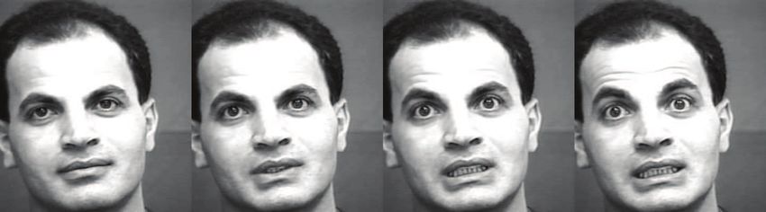
#".0%)'(*("$%&'("                                 events such as smiling and frowning, which must and can be
                                                                       detected and recognized independently of the background.
                                                                       Brown et al. [1] used the n-gram model for predictive typ-
                                                                       ing, i.e., predicting the next word from previous words.
                                                                       However, it is hard to apply their method to computer vi-
    1&%,'#*(2"                                                         sion, which does not have a well-defined language model
    )#-3#'"$%&'($"
                                                                       yet. Early detection has also been studied in the context
                                                                       of spam filtering, where immediate and irreversible deci-
Figure 2. Given a training time series that contains a complete        sions must be made whenever an email arrives. Assum-
event, we simulate the sequential arrival of training data and use     ing spam messages were similar to one another, Haider et
partial events as positive training examples. The red segments in-     al. [6] developed a method for detecting batches of spam
dicate the temporal extents of the partial events. We train a single   messages based on clustering. But visual events such as
event detector to recognize all partial events, but our method does    smiling or frowning cannot be detected and recognized just
more than augmenting the set of training examples.                     by observing the similarity between constituent frames, be-
                                                                       cause this characteristic is neither requisite nor exclusive to
oretically justified. In Sec. 3.2, we discuss two ways for             these events.
quantifying the loss for continuous detection on sequential                It is important to distinguish between forecasting and
data. We prove that, in both cases, the objective of the learn-        detection. Forecasting predicts the future while detection
ing formulation is to minimize an upper bound of the true              interprets the present. For example, financial forecast-
loss on the training data.                                             ing (e.g., [8]) predicts the next day’s stock index based on
    MMED has numerous benefits. First, MMED inher-                     the current and past observations. This technique cannot be
its the advantages of SOSVM, including its convex learn-               directly used for early event detection because it predicts the
ing formulation and its ability for accurate localization of           raw value of the next observation instead of recognizing the
event boundaries. Second, MMED, specifically designed                  event class of the current and past observations. Perhaps,
for early detection, is superior to SOSVM and other com-               forecasting the future is a good first step for recognizing
peting methods regarding the timeliness of the detection.              the present, but this two-stage approach has a disadvantage
Experiments on datasets of varying complexity, ranging                 because the former may be harder than the latter. For exam-
from sign language to facial expression and human actions,             ple, it is probably easier to recognize a partial smile than to
showed that our method often made faster detections while              predict when it will end or how it will progress.
maintaining comparable or even better accuracy.
                                                                       2.2. Event detection
2. Previous work                                                           This section reviews SVM, HMM, and SOSVM, which
  This section discusses previous work on early detection              are among the most popular algorithms for training event
and event detection.                                                   detectors. None of them are specifically designed for early
                                                                       detection.
2.1. Early detection                                                       Let (X1 , y1 ), · · · , (Xn , yn ) be the set of training time
                                                                       series and their associated ground truth annotations for the
    While event detection has been studied extensively in the
                                                                       events of interest. Here we assume each training sequence
literature of computer vision, little attention has been paid to
                                                                       contains at most one event of interest, as a training sequence
early detection. Davis and Tyagi [2] addressed rapid recog-
                                                                       containing several events can always be divided into smaller
nition of human actions using the probability ratio test. This
                                                                       subsequences of single events. Thus yi = [si , ei ] consists
is a passive method for early detection; it assumes that a
                                                                       of two numbers indicating the start and the end of the event
generative HMM for an event class, trained in a standard
                                                                       in time series Xi . Suppose the length of an event is bounded
way, can also generate partial events. Similarly, Ryoo [15]
                                                                       by lmin and lmax and we denote Y(t) be the set of length-
took a passive approach for early recognition of human ac-
                                                                       bounded time intervals from the 1st to the tth frame:
tivities; he developed two variants of the bag-of-words rep-
resentation to mainly address the computational issues, not             Y(t) = {y ∈ N2 |y ⊂ [1, t], lmin ≤ |y| ≤ lmax } ∪ {∅}.
timeliness or accuracy, of the detection process.
    Previous work on early detection exists in other fields,           Here | · | is the length function. For a time series X of
but its applicability in computer vision is unclear. Neill et          length l, Y(l) is the set of all possible locations of an event;
al. [11] studied disease outbreak detection. Their approach,           the empty segment, y = ∅, indicates no event occurrence.
like online change-point detection [3], is based on detecting          For an interval y = [s, e] ∈ Y(l), let Xy denote the subseg-
the locations where abrupt statistical changes occur. This             ment of X from frame s to e inclusive. Let g(X) denote the
technique, however, cannot be applied to detect temporal               output of the detector, which is the segment that maximizes
the detection score:                                                  To support early detection of events in time series data,
                                                                   we propose to use partial events as positive training exam-
                 g(X) = argmax f (Xy ; θ).                  (1)    ples (Fig. 2). In particular, we simulate the sequential arrival
                           y∈Y(l)
                                                                   of training data as follows. Suppose the length of Xi is li .
                                                                   For each time t = 1, · · · , li , let yti be the part of event yi
The output of the detector may be the empty segment, and if
                                                                   that has already happened, i.e., yti = yi ∩ [1, t], which is
it is, we report no detection. f (Xy ; θ) is the detection score
                                                                   possibly empty. Ideally, we want the output of the detector
of segment Xy , and θ is the parameter of the score function.
                                                                   on time series Xi at time t to be the partial event, i.e.,
Note that the detector searches over temporal scales from
lmin to lmax . In testing, this process can be repeated to                                        g(Xi[1,t] ) = yti .                 (3)
detect multiple target events, if more than one event occur.
     How is θ learned? Binary SVM methods learn θ by re-           Note that g(Xi[1,t] ) is not the output of the detector running
quiring the score of positive training examples to be greater      on the entire time series Xi . It is the output of the detector
than or equal to 1, i.e., f (Xiyi ; θ) ≥ 1, while constrain-       on the subsequence of time series Xi from the first frame to
ing the score of negative training examples to be smaller          the tth frame only, i.e.,
than or equal to −1. Negative examples can be selected
in many ways; a simple approach is to choose random                                     g(Xi[1,t] ) = argmax f (Xiy ).                (4)
segments of training time series that do not overlap with                                                 y∈Y(t)
positive examples. HMM methods define f (·, θ) as the
log-likelihood and learn θ that maximizes the total log-           From (3)-(4), the desired property of the score function is:
likelihood    of positive training examples, i.e., maximizing
P          i                                                                        f (Xiyi ) ≥ f (Xiy ) ∀y ∈ Y(t).                   (5)
    i f (X yi θ). HMM methods ignore negative training ex-
             ;                                                                                t

amples. SOSVM methods learn θ by requiring the score
                                                                   This constraint requires the score of the partial event yti to
of a positive training example Xiyi to be greater than the
                                                                   be higher than the score of any other time series segment y
score of any other segment from the same time series, i.e.,
                                                                   which has been seen in the past, y ⊂ [1, t]. This is illus-
f (Xiyi ; θ) > f (Xiy ; θ) ∀y 6= yi . SOSVM further requires
                                                                   trated in Fig. 3. Note that the score of the partial event is
this constraint to be well satisfied by a margin: f (Xiyi ; θ) ≥   not required to be higher than the score of a future segment.
f (Xiy ; θ) + ∆(yi , y) ∀y 6= yi , where ∆(yi , y) is the loss        As in the case of SOSVM, the previous constraint can
of the detector for outputting y when the desired output is        be required to be well satisfied by an adaptive margin. This
yi [12]. Though optimizing different learning objectives           margin is ∆(yti , y), the loss of the detector for outputting
and constraints, all of these aforementioned methods use           y when the desired output is yti (in our case ∆(yti , y) =
the same set of positive examples. They are trained to rec-             2|yti ∩y|
                                                                   1 − |yi |+|y|  ). The desired constraint is:
ognize complete events only, inadequately prepared for the                t

task of early detection.
                                                                              f (Xiyi ) ≥ f (Xiy ) + ∆(yti , y) ∀y ∈ Y(t).            (6)
                                                                                    t

3. Max-Margin Early Event Detectors                                This constraint should be enforced for all t = 1, · · · , li . As
   As explained above, existing methods do not train detec-        in the formulations of SVM and SOSVM, constraints are
tors to recognize partial events. Consequently, using these        allowed to be violated by introducing slack variables, and
methods for online prediction would lead to unreliable deci-       we obtain the following learning formulation:
sions as we will illustrate in the experimental section. This                             n
                                                                                1      CX i
section derives a learning formulation to address this prob-         minimize ||w||2 +       ξ,                                       (7)
lem. We use the same notations as described in Sec. 2.2.             w,b,ξ i ≥0 2      n i=1
                                                                                                                              ξi
3.1. Learning with simulated sequential data                                  s.t. f (Xiyi ) ≥ f (Xiy ) + ∆(yti , y) −        i
                                                                                          t                                   |yt |
                                                                                                                         µ    |yi |
  Let ϕ(Xy ) be the feature vector for segment Xy . We
consider a linear detection score function:                                                 ∀i, ∀t = 1, · · · , li , ∀y ∈ Y(t). (8)
                     T
                        w ϕ(Xy ) + b if y 6= ∅,
                                                                                                                            i
                                                                                                                            |y |
      f (Xy ; θ) =                                  (2)                Here | · | denotes the length function, and µ |yti | is
                        0                otherwise.
                                                                   a function ofthe proportion
                                                                                                 of the event that has occurred
                                                                                   |yti |
Here θ = (w, b), w is the weight vector and b is the bias          at time t. µ |yi | is a slack variable rescaling factor and
term. From now on, for brevity, we use f (Xy ) instead of          should correlate with the importance of correctly detecting
f (Xy ; θ) to denote the score of segment Xy .                     at time t whether the event yi has happened. µ(·) can be any
si                            t            ei                                          t       t     t      t     t
 Xi

                 #$%&""                                        01)#3'&'""      +,&,-'""
                 %'()'*&"                   #$-2$3""
                                  yti       '4'*&"
                                                                 '4'*&"      %'()'*&"

 "01*%&-$/*&5"
  f (Xiyi )> f (Xy
                 i
                   past
                        )
         t

                                                                                                                        $%&'(%$#&)*(%#+,-).*-# f (·)
                                        .'%/-'."%01-'"+,*021*" f (·)
                                                                                           Figure 4. Monotonicity requirement – the detection score of a
Figure 3. The desired score function for early event detection: the                        partial event cannot exceed the score of an encompassing partial
complete event must have the highest detection score, and the de-                          event. MMED provides a principled mechanism to achieve this
tection score of a partial event must be higher than that of any                           monotonicity, which cannot be assured by a naive solution that
segment that ends before the partial event. To learn this function,                        simply augments the set of training examples.
we explicitly consider partial events during training. At time t, the
score of the truncated event (red segment) is required to be higher                        not started. Constraint (10) requires successful recognition
than the score of any segment in the past (e.g., blue segment);
                                                                                           of partial events. Constraint (11) trains the detector to accu-
however, it is not required to be higher than the score of any future
segment (e.g., green segment). This figure is best seen in color.
                                                                                           rately localize the temporal extent of the partial events.
                                                                                               The proposed learning formulation Eq. (7) is convex, but
arbitrary non-negative function, and in general, it should be                              it contains a large number of constraints. Following [17],
a non-decreasing function in (0, 1]. In our experiments, we                                we propose to use constraint generation in optimization, i.e.,
found the following piece-wise linear function a reasonable                                we maintain a smaller subset of constraints and iteratively
choice: µ(x) = 0 for 0 < x ≤ α; µ(x) = (x − α)/(β −                                        update it by adding the most violated ones. Constraint gen-
α) for α < x ≤ β; and µ(x) = 1 for β < x ≤ 1 or                                            eration is guaranteed to converge to the global minimum. In
x = 0. Here, α and β are tunable parameters. µ(0) =                                        our experiments described in Sec. 4, this usually converges
µ(1) emphasizes that true rejection is as important as true                                within 20 iterations. Each iteration requires minimizing a
detection of the complete event.                                                           convex quadratic objective. This objective is optimized us-
    This learning formulation is an extension of SOSVM.                                    ing Cplex1 in our implementation.
From this formulation, we obtain SOSVM by not simulat-
ing the sequential arrival of training data, i.e., to set t = li                           3.2. Loss function and empirical risk minimization
instead of t = 1, · · · , li in Constraint (8). Notably, our                                   In Sec. 3.1, we have proposed a formulation for training
method does more than augmenting the set of training ex-                                   early event detectors. This section provides further discus-
amples; it enforces the monotonicity of the detector func-                                 sion on what exactly is being optimized. First, we briefly
tion, as shown in Fig. 4.                                                                  review the loss of SOSVM and its surrogate empirical risk.
    For a better understanding of Constraint (8), let us ana-
                                                                                           We then describe two general approaches for quantifying
lyze the constraint without the slack variable term and break
it into three cases: i) t < si (event has not started); ii)                                the loss of a detector on sequential data. In both cases, what
t ≥ si , y = ∅ (event has started; compare the partial                                     Eq. (7) minimizes is an upper bound on the loss.
event against the detection threshold); iii) t ≥ si , y 6= ∅                                   As previously explained, ∆(y, ŷ) is the function that
(event has started; compare the partial event against any                                  quantifies the loss associated with a prediction ŷ, if the
non-empty segment). Recall f (X∅ ) = 0 and yti = ∅ for                                     true output value is y. Thus, in the setting of offline de-
t < si , cases (i), (ii), (iii) lead to Constraints (9), (10), (11),                       tection, the loss of a detector g(·) on a sequence-event pair
respectively:                                                                              (X, y) is quantified as ∆(y, g(X)). Suppose the sequence-
  f (Xiy ) ≤ −1 ∀y ∈ Y(si − 1) \ {∅},                                                (9)
                                                                                           event pairs (X, y) are generated according to some distri-
                                                                                           bution  P (X, y), the loss of the detector g is R∆  true (g) =
  f (Xiyi )   ≥ 1 ∀t ≥ s ,   i
                                                                                   (10)    R
                                                                                                   ∆(y,  g(X))dP   (X, y).  However,   P  is unknown    so
        t
                                                                                             X ×Y
  f (Xiyi )   ≥   f (Xiy )   +   ∆(yti , y)            i
                                              ∀t ≥ s , y ∈ Y(t) \ {∅}. (11)                the performance of g(.) is described by the empirical risk
        t

Constraint (9) prevents false detection when the event has                                   1 www-01.ibm.com/software/integration/optimization/cplex-optimizer/
on the training data {(Xi , yi )}, assuming they are gener-          Area under the ROC curve: Consider testing a detec-
ated i.i.d according to P . The empirical risk is R∆emp (g) =    tor on a set of time series. The False Positive Rate (FPR) of
 1 Pn         i        i                                         the detector is defined as the fraction of time series that the
n    i=1  ∆(y   , g(X    )). It has been shown  that  SOSVM
minimizes an upper bound on the empirical risk R∆    emp [17].
                                                                 detector fires before the event of interest starts. The True
   Due to the nature of continual evaluation, quantifying        Positive Rate (TPR) is defined as the fraction of time series
the loss of an online detector on streaming data requires        that the detector fires during the event of interest. A detec-
aggregating the losses evaluated throughout the course of        tor typically has a detection threshold that can be adjusted
the data sequence. Let us consider the loss associated with      to trade off high TPR for low FPR and vise versa. By vary-
a prediction y = g(Xi[1,t] ) for time series Xi at time t        ing this detection threshold, we can generate the ROC curve
                i
                  |y |                                           which is the function of TPR against FPR. We use the area
as ∆(yti , y)µ |yti | . Here ∆(yti , y) accounts for the dif-    under the ROC for evaluating the detector accuracy.
                                                        i
ference
   i between the output y and true truncated event yt .            AMOC curve: To evaluate the timeliness of detection
    |yt |                                                        we used Normalized Time to Detection (NTtoD) which is
µ |yi | is the scaling factor; it depends on how much the
                                                                 defined as follows. Given a testing time series with the event
temporal event yi has happened. Two possible ways for ag-
                                                                 of interest occurs from s to e. Suppose the detector starts to
gregating these loss quantities is to use their maximum or
                                                                 fire at time t. For a successful detection, s ≤ t ≤ e, we de-
average. They lead to two different empirical risks for a set
                                                                 fine the NTtoD as the fraction of event that has occurred,
of training time series:                                               t−s+1
                                                                 i.e., e−s+1  . NTtoD is defined as 0 for a false detection
               n                              i              (t < s) and ∞ for a false rejection (t > e). By adjust-
            1X                                  |yt |
 R∆,µ
  max (g) =               i        i
                 max ∆(yt , g(X[1,t] ))µ               ,         ing the detection threshold, one can achieve lower NTtoD
            n i=1 t                             |yi |
                                                                 at the cost of higher FPR and vice versa. For a complete
               n                               i             characteristic picture, we varied the detection threshold and
            1X                                   |yt |
R∆,µ
 mean (g) =      mean  ∆(y  i
                            t , g(X  i
                                     [1,t] ))µ           .       plotted the curve of NToD versus FPR. This is referred as
            n i=1 t                              |yi |
                                                                 the Activity Monitoring Operating Curve (AMOC) [4].
                                                                     F1-score curve: The ROC and AMOC curves, how-
   In the following, we state and prove a proposition that
establishes that the learning formulation given in Eq. 7 min-    ever, do not provide a measure for how well the de-
                                                                 tector can localize the event of interest. For this pur-
imizes an upper bound of the above two empirical risks.
                                                                 pose, we propose to use the frame-based F 1-scores. Con-
   Proposition: Denote by ξ∗ (g) the optimal solution
                                                                 sider running a detector on a times series. At time t
        Pn variables in Eq. (7) for a given detector g,
of the slack
                                                                 the detector output the segment y while the ground truth
then n1 i=1 ξ i∗ is an upper bound on the empirical risks
                                                                 (possibly) truncated event is y∗ . The F 1-score is de-
R∆,µ              ∆,µ
  max (g) and Rmean (g).
                                                                 fined as the harmonic mean of precision and recall values:
   Proof: Consider Constraint (8) with y = g(Xi[1,t] ) and       F 1 := 2 PPrecision+Recall
                                                                              recision∗Recall
                                                                                              , with P recision := |y∩y
                                                                                                                           ∗
                                                                                                                             |
                                                                                                                               and
                                                                                                                       |y|
together with the fact that f (Xig(Xi ) ) ≥ f (Xiyi ), we
                                                                 Recall := |y∩y     |
                                                                                  ∗

                                    i[1,t]       t
                                                                               |y∗ | . For a new test time series, we can simu-
                                     |yt |                       late the sequential arrival of data and record the F 1-scores
have ξ ≥ ∆(yt , g(X[1,t] ))µ |yi | ∀t. Thus ξ i∗ ≥
       i∗          i       i
                            i
                             |y |             Pn                 as the event of interest unroll from 0% to 100%. We refer
maxt {∆(yti , g(Xi[1,t] ))µ |yti | }. Hence n1 i=1 ξ i∗ ≥        to this as the F1-score curve.
R∆,µ           ∆,µ
  max (g) ≥ Rmean (g). This completes the proof of the           4.2. Synthetic data
proposition. This proposition justifies the objective of the
learning formulation.                                               We first validated the performance of MMED on a
                                                                 synthetically generated dataset of 200 time series. Each
4. Experiments                                                   time series contained one instance of the event of inter-
                                                                 est, signal 5(a).i, and several instances of other events, sig-
    This section describes our experiments on several pub-       nals 5(a).ii–iv. Some examples of these time series are
licly available datasets of varying complexity.                  shown in Fig. 5(b). We randomly split the data into training
                                                                 and testing subsets of equal sizes. During testing we sim-
4.1. Evaluation criteria
                                                                 ulated the sequential arrival of data and recorded the mo-
   This section describes several criteria for evaluating the    ment that MMED started to detect the start of the event of
accuracy and timeliness of detectors. We used the area un-       interest. With 100% precision, MMED detected the event
der the ROC curve for accuracy comparison, Normalized            when it had completed 27.5% of the event. For comparison,
Time to Detection (NTtoD) for benchmarking the timeli-           SOSVM required observing 77.5% of the event for a posi-
ness of detection, and F 1-score for evaluating localization     tive detection. Examples of testing time series and results
quality.                                                         are depicted in Fig. 5(b). The events of interest are drawn in
i ii 0 50 100 150 200
proach; the window size was fixed to the average length of
4 4 4
2 2 2 the I-love-you sentences.
0 0 0 Inspired by the high recognition rate of HMM, we con-
0 50 0 50 0 50 100 150 200
iii iv structed the feature representation for SVM-based detec-
4 4 4
2
tors (SOSVM and MMED) as follows. We first trained a
2 2
0 0 0 Gaussian Mixture Model of 20 Gaussians for the frames
0 50 0 50 0 50 100 150 200 extracted from the I-love-you sentences. Each frame was
(a) (b) then associated with a 20 × 1 log-likelihood vector. We re-
Figure 5. Synthetic data experiment. (a): time series were created tained the top three values of this vector, zeroing out the
by concatenating the event of interest (i) and several instances of other values, to create a frame-level feature representation.
other events (ii)–(iv). (b): examples of testing time series; the This is often referred to as a soft quantization approach. To
solid vertical red lines mark the moments that our method starts to compute the feature vector for a given window, we divided
detect the event of interest while the dash blue lines are the results the window into two roughly equal halves, the mean feature
of SOSVM. vector of each half was calculated, and the concatenation of
these mean vectors was used as the feature representation of
green and the solid vertical red lines mark the moments that the window.
our method started to detect these events. The dash verti- A naive strategy for early detection is to use truncated
cal blue lines are the results of SOSVM. Notably, this result events as positive examples. For comparison, we imple-
reveals an interesting capability of MMED. For the time se- mented Seg-[0.5,1], a binary SVM that used the first halves
ries in this experiment, the change in signal values from 3 of the I-love-you sentences in addition to the full sentences
to 1 is exclusive to the target events. MMED was trained to as positive training examples. Negative training examples
recognize partial events, it implicitly discovered this unique were random segments that had no overlapping with the I-
behavior, and it detected the target events as soon as this love-you sentences.
behavior occurred. In this experiment, we represented each We repeated our experiment 10 times and recorded the
time series segment by the L2 -normalized histogram of sig- average performance. Regarding the detection accuracy, all
nal values in the segment (normalized to have unit norm). methods except SVM-[0.5,1] performed similarly well. The
We used linear SVM with C = 1000, α = 0, β = 1. ROC areas for HMM, SVM-[0.5,1], SOSVM, and MMED
were 0.97, 0.92, 0.99, and 0.99, respectively. However,
4.3. Auslan dataset – Australian sign language when comparing the timeliness of detection, MMED out-
This section describes our experiments on a publicly performed the others by a large margin. For example, at
available dataset [7] that contains 95 Auslan signs, each 10% false positive rate, our method detected the I-love-you
with 27 examples. The signs were captured from a native sentence when it observed the first 37% of the sentence. At
signer using position trackers and instrumented gloves; the the same false positive rate, the best alternative method re-
location of two hands, the orientation of the palms, and the quired seeing 62% of the sentence. The full AMOC curves
bending of the fingers were recorded. We considered de- are depicted in Fig. 6(a). In this experiment, we used linear
tecting the sentence “I love you” in monologues obtained SVM with C = 1, α = 0.25, β = 1.
by concatenating multiple signs. In particular, each mono-
4.4. Extended Cohn-Kanade dataset – expression
logue contained an I-love-you sentence which was pre-
ceded and succeeded by 15 random signs. The I-love-you The Extended Cohn-Kanade dataset (CK+) [10] contains
sentence was ordered concatenation of random samples of 327 facial image sequences from 123 subjects performing
three signs: “I”, “love”, and “you”. We created 100 training one of seven discrete emotions: anger, contempt, disgust,
and 200 testing monologues from disjoint sets of sign sam- fear, happiness, sadness, and surprise. Each of the se-
ples; the first 15 examples of each sign were used to create quences contains images from onset (neutral frame) to peak
training monologues while the last 12 examples were used expression (last frame). We considered the task of detecting
for testing monologues. The average lengths and standard negative emotions: anger, disgust, fear, and sadness.
deviations of the monologues and the I-love-you sentences We used the same representation as [10], where each
were 1836 ± 38 and 158 ± 6 respectively. frame is represented by the canonical normalized appear-
Previous work [7] reported high recognition perfor- ance feature, referred as CAPP in [10]. For comparison
mance on this dataset using HMMs. Following their suc- purposes, we implemented two frame-based SVMs: Frm-
cess, we implemented a continuous density HMM for I- peak was trained on peak frames of the training sequences
love-you sentences. Our HMM implementation consisted while Frm-all was trained using all frames between the on-
of 10 states, each was a mixture of 4 Gaussians. To use set and offset of the facial action. Frame-based SVMs can
the HMM for detection, we adopted a sliding window ap- be used for detection by classifying individual frames. In1 1 1
HMM Frm−peak
0.9 Seg−[0.5,1] 0.9 Frm−all 0.9
SOSVM SOSVM
0.8 0.8 0.8
MMED MMED
Normalized Time to Detect
Normalized Time to Detect
0.7 0.7 0.7
0.6 0.6 0.6
F1 score
0.5 0.5 0.5
0.4 0.4 0.4
0.3 0.3 0.3
Seg−[1]
0.2 0.2 0.2
Seg−[0.5,1]
0.1 0.1 0.1 SOSVM
MMED
0 0 0
0 0.2 0.4 0.6 0.8 1 0 0.2 0.4 0.6 0.8 1 0 0.2 0.4 0.6 0.8 1
False Positive Rate False Positive Rate Fraction of the event seen
(a) Auslan, AMOC (b) CK+, AMOC (c) Weizmann, F1 curve
Figure 6. Performance curves. (a, b): AMOC curves on Auslan and CK+ datasets; at the same false positive rate, MMED detects the event
of interest sooner than the others. (c): F1-score curves on Weizmann dataset; MMED provides better localization for the event of interest,
especially when the fraction of the event observed is small. This figure is best seen in color.
disgust
contrast, SOSVM and MMED are segment-based. Since
a facial expression is a deviation of the neutral expression,
we represented each segment of an emotion sequence by the
difference between the end frame and the start frame. Even
0.00 0.53 0.73 1.00
though the start frame was not necessary a neutral face, this (a) fear
representation led to good recognition results.
We randomly divided the data into disjoint training and
testing subsets. The training set contained 200 sequences
with equal numbers of positive and negative examples. For
reliable results, we repeated our experiment 20 times and 0.00 0.44 0.62 1.00
(b)
recorded the average performance. Regarding the detec-
tion accuracy, segment-based SVMs outperformed frame- Figure 7. Disgust (a) and fear (b) detection on CK+ dataset. From
based SVMs. The ROC areas (mean and standard deviation) left to right: the onset frame, the frame at which MMED fires, the
for Frm-peak, Frm-all, SOSVM, MMED are 0.82 ± 0.02, frame at which SOSVM fires, and the peak frame. The number in
0.84 ± 0.03, 0.96 ± 0.01, and 0.97 ± 0.01, respectively. each image is the corresponding NTtoD.
Comparing the timeliness of detection, our method was sig-
nificantly better than the others, especially at low false pos- was represented by the ID of the corresponding codebook
itive rate. For example, at 10% false positive rate, Frm- entry and each segment of a time series was represented by
peak, Frm-all, SOSVM, and MMED can detect the expres- the histogram of temporal words associated with frames in-
sion when it completes 71%, 64%, 55%, and 47% respec- side the segment.
tively. Fig. 6(b) plots the AMOC curves, and Fig. 7 displays We trained a detector for each action class, but consid-
some qualitative results. In this experiment, we used a lin- ered them one by one. We created 9 long video sequences,
ear SVM with C = 1000, α = 0, β = 0.5. each composed of 10 videos of the same person and had the
event of interest at the end of the sequence. We performed
4.5. Weizmann dataset – human action
leave-one-out cross validation; each cross validation fold
The Weizmann dataset contains 90 video sequences of 9 trained the event detector on 8 sequences and tested it on
people, each performing 10 actions. Each video sequence the leave-out sequence. For the testing sequence, we com-
in this dataset only consists of a single action. To measure puted the normalized time to detection at 0% false positive
the accuracy and timeliness of detection, we performed ex- rate. This false positive rate was achieved by raising the
periments on longer video sequences which were created threshold for detection so that the detector would not fire
by concatenating existing single-action sequences. Follow- before the event started. We calculated the median normal-
ing [5], we extracted binary masks and computed Euclidean ized time to detection across 9 cross validation folds and
distance transform for frame-level features. Frame-level averaged these median values across 10 action classes; the
feature vectors were clustered using k-means to create a resulting values for Seg-[1], Seg-[0.5,1], SOSVM, MMED
codebook of 100 temporal words. Subsequently, each frame are 0.16, 0.23, 0.16, and 0.10 respectively. Here Seg-[1] wasa segment-based SVM, trained to classify the segments cor- References
responding to the complete action of interest. Seg-[0.5,1]
[1] P. F. Brown, P. V. deSouza, R. L. Mercer, V. J. D. Pietra, and
was similar to Seg-[1], but used the first halves of the ac-
J. C. Lai. Class-based n-gram models of natural language.
tion of interest as additional positive examples. For each Computational Linguistics, 18(4), 1992.
testing sequence, we also generated a F1-score curve as de- [2] J. Davis and A. Tyagi. Minimal-latency human action recog-
scribed in Sec. 4.1. Fig. 6(c) displays the F 1-score curves nition using reliable-inference. Image and Vision Comput-
of all methods, averaged across different actions and dif- ing, 24(5):455–472, 2006.
ferent cross-validation folds. MMED significantly outper- [3] F. Desobry, M. Davy, and C. Doncarli. An online kernel
formed the other methods. The superiority of MMED over change detection algorithm. IEEE Transactions on Signal
SOSVM was especially large when the fraction of the event Processing, 53(8):2961–2974, 2005.
observed was small. This was because MMED was trained [4] T. Fawcett and F. Provost. Activity monitoring: Notic-
to detect truncated events while SOSVM was not. Though ing interesting changes in behavior. In Proceedings of the
SIGKDD Conference on Knowledge Discovery and Data
also trained with truncated events, Seg-[0.5,1] performed
Mining, 1999.
relatively poor because it was not optimized to produce cor-
[5] L. Gorelick, M. Blank, E. Shechtman, M. Irani, and R. Basri.
rect temporal extent of the event. In this experiment, we Actions as space-time shapes. Transactions on Pattern Anal-
used the linear SVM with C = 1000, α = 0, β = 1. ysis and Machine Intelligence, 29(12):2247–2253, 2007.
[6] P. Haider, U. Brefeld, and T. Scheffer. Supervised clustering
of streaming data for email batch detection. In International
5. Conclusions Conference on Machine Learning, 2007.
[7] M. Kadous. Temporal classification: Extending the classi-
This paper addressed the problem of early event detec- fication paradigm to multivariate time series. PhD thesis,
tion. We proposed MMED, a temporal classifier specialized 2002.
in detecting events as soon as possible. Moreover, MMED [8] K.-J. Kim. Financial time series forecasting using support
provides localization for the temporal extent of the event. vector machines. Neurocomputing, 55(1-2):307–319, 2003.
MMED is based on SOSVM, but extends it to anticipate se- [9] T. Lan, Y. Wang, and G. Mori. Discriminative figure-centric
quential data. During training, we simulate the sequential models for joint action localization and recognition. In In-
arrival of data and train a detector to recognize incomplete ternational Conference on Computer Vision, 2011.
[10] P. Lucey, J. F. Cohn, T. Kanade, J. Saragih, Z. Ambadar, and
events. It is important to emphasize that we train a sin-
I. Matthews. The extended Cohn-Kanade dataset (CK+): A
gle event detector to recognize all partial events and that complete dataset for action unit and emotion-specified ex-
our method does more than augmenting the set of training pression. In CVPR Workshop on Human Communicative Be-
examples. Our method is particularly suitable for events havior Analysis, 2010.
which cannot be reliably detected by classifying individ- [11] D. Neill, A. Moore, and G. Cooper. A Bayesian spatial scan
ual frames; detecting this type of events requires pooling statistic. In Neural Information Processing Systems. 2006.
information from a supporting window. Experiments on [12] M. H. Nguyen, T. Simon, F. De la Torre, and J. Cohn. Action
datasets of varying complexity, from synthetic data and sign unit detection with segment-based SVMs. In IEEE Confer-
language to facial expression and human actions, showed ence on Computer Vision and Pattern Recognition, 2010.
that our method often made faster detections while main- [13] S. M. Oh, J. M. Rehg, T. Balch, and F. Dellaert. Learn-
taining comparable or even better accuracy. Furthermore, ing and inferring motion patterns using parametric segmen-
tal switching linear dynamic systems. International Journal
our method provided better localization for the target event,
of Computer Vision, 77(1–3):103–124, 2008.
especially when the fraction of the seen event was small. In
[14] A. Patron-Perez, M. Marszalek, A. Zisserman, and I. Reid.
this paper, we illustrated the benefits of our approach in the High Five: Recognising human interactions in TV shows. In
context of human activity analysis, but our work can be ap- Proceedings of British Machine Vision Conference, 2010.
plied to many other domains. The active training approach [15] M. Ryoo. Human activity prediction: Early recognition of
to detect partial temporal events can be generalized to detect ongoing activities from streaming videos. In Proceedings of
truncated spatial objects [18]. International Conference on Computer Vision, 2011.
[16] S. Satkin and M. Hebert. Modeling the temporal extent of
Acknowledgments: This work was supported by the National Sci-
actions. In European Conference on Computer Vision, 2010.
ence Foundation (NSF) under Grant No. RI-1116583. Any opin-
[17] I. Tsochantaridis, T. Joachims, T. Hofmann, and Y. Al-
ions, findings, and conclusions or recommendations expressed in
tun. Large margin methods for structured and interdependent
this material are those of the author(s) and do not necessarily re-
output variables. Journal of Machine Learning Research,
flect the views of the NSF. The authors would like to thank Y. Shi
6:1453–1484, 2005.
for the useful discussion on early detection, L. Torresani for the
[18] A. Vedaldi and A. Zisserman. Structured output regression
suggestion of F1 curves, M. Makatchev for the discussion about
for detection with partial truncation. In Proceedings of Neu-
AMOC, T. Simon for AU data, and P. Lucey for providing CAPP
ral Information Processing Systems, 2009.
features for the CK+ dataset.You can also read