Real-time on-Board Manycore Implementation of a Health Monitoring System: Lessons Learnt - ERTS 2018
←
→
Page content transcription
If your browser does not render page correctly, please read the page content below
1

 Real-time on-Board Manycore Implementation
of a Health Monitoring System: Lessons Learnt
                                  Moustapha Lo, Nicolas Valot
                                      Airbus Helicopters
                             Florence Maraninchi, Pascal Raymond
       Univ. Grenoble Alpes, CNRS, Grenoble INP∗ , VERIMAG, 38000 Grenoble, France

    Abstract—Maintenance has long been a predomi-                  The current implementation of the HMS is not
nant activity in the industrial sector. Measuring and           embedded in the helicopter. An embedded acqui-
analyzing physical signals on the machines allows to            sition unit records the vibrations during the flight
provide a diagnosis on their health state. The more             without any loss (the recording frequency must be
recent Health Monitoring Systems (HMS) allow to
                                                                at least equal to the sensors sampling frequency).
optimize the maintenance operations by performing
preventive maintenance. The existing HMS are based
                                                                Signal processing algorithms that define the various
on various signal-processing algorithms applied to              health indicators are computed on-ground. This
vibration data gathered during flights, in order to             requires a huge storage capacity, and a high network
compute health indicators. The computation of the               bandwidth for data offloading.
indicators is done on-ground, once a full data set has             According to [7], the helicopter S-92 designed by
been offloaded.                                                 Sikorsky is, since March, 2017, the first helicopter
    In this paper, we report on experiments made                that has the ability to transmit in real-time raw
to turn these on-ground computations into on-board
                                                                vibration data. Vibration data are transmitted to
real-time computations, using a many-core processor.
                                                                a ground support team that performs maintenance
There are two main issues to be addressed: (i) the
management of the flow of inputs from sensors;                  operations. In others words, the real-time imple-
(ii) the (hopefully tolerable) errors we make when              mentation is not embedded in the helicopter. It is a
transforming an on-ground algorithm that can treat              real-time but on-ground computation.
data globally, into an on-board real-time algorithm                We study how to provide an on-line embedded
that is necessarily incremental. We show that the               version of the existing on-ground HMS application
error is indeed acceptable.                                     for several reasons. First, the existing application
  Index terms— on-ground, on-board, real-time,                  runs on the PC of the helicopter operator/customer,
many-core, global or incremental algorithms, Health             and cannot be trusted entirely by the helicopter
Monitoring Systems.                                             manufacturer, who has to recommend periodic and
                                                                potentially costly maintenance sessions. If the HMS
                   I. I NTRODUCTION                             is computed on-line, it will inherit the critical-
   The HMS function monitors the vibration of                   ity level of the on-board computing unit, and be
the helicopter system components like gear boxes,               more reliable for the manufacturer. It is one of
transmission shafts, rotors, and bearings. Vibrations           the enablers to replace periodic maintenance with
are measured by sensors and the data are then                   predictive maintenance. Second, it will save time
provided to a computation unit that performs signal             between flights, and therefore increase the heli-
processing to compute health indicators. Some of                copter availability.
the HMS indicators are intended to detect mechan-                  Our purpose is to build an embedded real-time
ical fatigue occurring during helicopter operation.             implementation of the HMS. The health indicators
The interpretation of the indicators in terms of                will be computed on-board. Because of the comput-
mechanical defects, and the very choice of the                  ing requirements of the signal processing algorithms
indicators to be computed, are based on previous                involved, it is necessary to choose an embedded
expertise and empirical studies of the helicopters.             processor that guarantees high performance and the
                                                                ability to be used in certified equipment. According
  This work was supported by the CAPACITES research
                                                                to [1], the benefits of the MPPA family of proces-
project, supported by the French authorities through the “In-
vestissements d’Avenir” program.                                sors for critical real-time systems are: predictable
  * Institute of Engineering Univ. Grenoble Alpes               computation and responses times, low power, and
2
high performance. speed ratio w.r.t. the speed of the reference shaft it
The first challenge is the need to transform a depends on.
global algorithm into an incremental one. With the Figure 1 shows two reference shafts: the main
on-ground global algorithms, we consider the full and the tail rotors. Two monitored shafts are con-
data set to compute indicators (e.g., we may use a nected to the main rotor: IGB and OGB, with a
global average). The embedded real-time algorithm rotational speed ratio rm = 2 (they rotate twice
should be able to treat data as soon as they become faster). Two monitored shafts are connected to the
available, because it is impossible to store them tail rotor, TDS1 (Tail Drive Shaft left) and TDS2
before computing the indicators. The transformation (Tail Drive Shaft right), with a rotational speed ratio
of the algorithms will necessarily introduce some rt = 4 (they rotate 4 times faster).
errors, w.r.t. the on-ground global algorithm con-
sidered as the reference implementation. phase sensor
The second challenge is the real-time aspect: we accelerometer
main
focus on inputs, and the constraint of computing rotor
connection/speedup ratio
health-indicators sufficiently fast with respect to the
monitored shaft
volume of data determined by the input frequency
rm = 2
and the number of sensors.
In this paper we are not concerned by the tech- TDS1 tail rotor
IGB
niques that can be used to map the entire compu-
tations onto the computing units of the many-core OGB rt = 4
TDS2
processor. We carefully examine the whole chain
between sensor data and the indicators, through
the acquisition card, the bus connecting it to the Fig. 1: The Mechanical System and the sensors
processor, and the I/O interface of the processor. We
perform experiments with a simple mapping, and B. Acquisition Unit
derive various dimensioning indications, related to The acquisition unit is a piece of equipment that
the number of sensors, the sampling frequency (i.e., acquires the sensor data, and provides a flow of
the volume of data), and the number of indicators inputs for the computations. During a flight, it per-
to be computed. forms one or several acquisition sessions. A session
Section II describes the mechanical system, the is characterized by the choice of enabled accelerom-
sensors, and the maintenance decisions. Section III eters, the sampling frequency, and the sampling
details the different steps of the existing global size (number of samples per accelerometer acquired
algorithm used on-ground to compute health in- during the session). Each session is stored in a file
dicators. Section IV explains the problems faced and contains vibration samples of accelerometers
when transforming the existing algorithms into real- and tops from the phase sensor. Suppose we have
time embedded ones. Section V focuses on the only one phase sensor on the tail rotor, and one
architecture of the many-core processor MPPA-256. accelerometer on a rotating element with speed
Section VI reports on our implementation experi- ratio 4. The acquisition unit builds a sequence of
ments on the Kalray MPPA processor and finally tuples (v, t), where v is a vibration measure, and t
section VII lists lessons learnt and further work. is a Boolean, corresponding to the phase sensor.
The sequence of values occurring between two
II. M ECHANICAL S YSTEM , ACQUISITION U NIT, successive rising edges of t corresponds to the data
AND I NDICATORS A NALYSIS gathered for 4 revolutions of the monitored element.
The sampling frequency is in the range [1−31]k Hz.
A. Mechanical System The top is very important: although the speed of the
The mechanical system involves phase sensors rotating parts varies, the top allows the measures to
and accelerometers. Phase sensors are placed on be gathered per revolution of the monitored rotating
reference shafts. They observe a tooth placed on part.
the rotating part, in such a way that a top signal Moreover, the data are not delivered one sample
can be generated at each revolution, and sent to at a time. The acquisition unit fills a buffer (the
the rest of the system. Various accelerometers are size of which corresponds to 100 ko, typically).
placed on the rotating elements to monitor their vi- The buffer is then read by the computation part,
brations. Each monitored shaft has a fixed rotational sufficiently often so as not to lose samples. In3
the on-line version, the size of the data packets based on that observation, and performed after date
exchanged between the acquisition card and the 4. This is the reason why the OM1 indicator then
many-core processors has to be large enough, to decreases to 1.5g at date 5.
ensure that the over-cost of the transmission w.r.t. There is a trend towards using machine learning
to the payload is not too big. We examine this point techniques in order to replace the human diagnosis
in section VI-B. based on indicators by automatic decision meth-
ods [5]. The machine learning algorithms should
C. Computation of the HMS Indicators and Main- be trained with existing data from previous flights,
tenance Decisions and corresponding recorded human decisions.
For a given acquisition file and monitored shaft,
the existing off-line application computes a set of D. Evaluation Criteria for the Online Version
frequency indicators (OM1, OM2, ...) and tem- When transforming the on-ground algorithms
poral indicators (RMS,RMSR,Kurtosis, Skewness, into embedded real-time ones, we need to compare
...). For instance, OM1 allows to detect the mis- the new version to a reference one. What really
alignment of the monitored shaft (i.e., the relative matters is the decision taken by the human operator,
position deviation of the shaft from the collinear based on the evolution of the indicators as shown
rotation axis). Maintenance decisions are taken by on Fig. 2. The ultimate criteria is that, for the same
considering the evolution of indicators at successive data, the on-line version leads to the same decisions
acquisition dates. Acquisition dates can come from as the on-ground global version.
the same flight, or different flights, but always at the However, in the experiments reported in this
same helicopter flight regime, in order to be com- paper, we cannot only look at the final result,
parable. The helicopter regime is characterized by because we cannot ask the human operators what
a value IAS (Indicator Air Speed) between IAS min they would have decided based on the results we
and IAS max, which are configuration parameters compute. Instead, we carefully tracked all the steps
for the helicopter. of the algorithms (from the acquisition of sensor
Figure 2 illustrates the evolution of the indicator data to the computation of the indicators), in order
OM1 depending on the acquisition date. The x axis to detect potential discrepancies as early as pos-
represents the acquisition dates from 1 to 5, and the sible in the complete chain. This provides general
y axis gives the indicator OM1 (in g unit). guidelines on what to check when transforming any
on-ground global algorithm into on-line real-time
OM1 programs. The differences between the two versions
(g)
my have different impact depending on the nature
Threshold
of the indicators (temporal of frequency domains,
2
typically).
III. E XISTING GLOBAL ALGORITHM
maintenance
1 The existing global algorithm uses as inputs
the vibration data acquired during the flight. The
acquisition file contains vibration samples of ac-
date1 date2 date3 date4 date5 celerometers and the tops of the phase sensor. The
Fig. 2: Evolution of indicator OM1, for a given global algorithm is used to calculate the raw signal
flight regime. that will be used as inputs to compute the indicators.
The human operators are provided with a web A. Steps of the Global algorithm
interface that essentially shows pictures similar to There are several shafts to monitor and the in-
that of Fig. 2. A threshold value is set, based on dicators which allow to monitor the vibration level
human expertise. It may depend on a particular are computed using samples of each revolution of a
helicopter and operating conditions. If the indicator given shaft. Because indicators are associated with
is above the threshold, it means a defect has been monitored shaft revolutions, we must be able to
detected. In figure 2, the threshold has been set to delimit the beginning and the end of each revolution
2g . The value of the indicator has been above 2g at of the monitored shaft. This operation is done by
dates 3 and 4. A maintenance operation was decided first detecting the reference tops in the acquisition4
of a new revolution of the reference shaft (main
or tail rotor). The rotation speed of the reference
shaft is not constant. That is why, in figure 3, the
discrete time scale given by the samples interval between two rising edges is not constant.
For example, the 2nd revolution of the reference
shaft is longer than the 1st revolution. It means the
phase sensor shaft slows down during the 2nd revolution. A lower
speed of the reference shaft implies a higher number
1st rev. 2nd rev. 3rd rev. of samples. Here, in particular, the first revolution
has 22 samples, while the second one has 25.
2) Estimating the tops of the monitored shaft
Estimated revolutions of the monitored shaft (r = 2)
(case of an integer ratio): Once the positions of
the reference revolutions have been detected, each
s1
s1
of them has to be split into r equal parts, where r
s1 is the speed ratio of the monitored shaft (as shown
s2 on Figure 1).
Estimated revolutions of the monitored shaft (r = 2.3) On figure 3, the first case corresponds to the
Fig. 3: Estimated tops of the monitored shaft with integer ratio r = 2. Each revolution is split into
integer or non integer ratational speed ratios. 2 equal parts.
Notice that dividing the reference shaft revolution
into equal monitored shaft revolutions implies that
we consider the speed to be constant during one ref-
file, then estimating the position of the tops of the erence revolution (some knowledge about previous
monitored shaft, knowing the rotational speed ratio revolutions and a bound on the acceleration could be
between the reference rotor and the monitored shaft. used to perform a more accurate division, but the
This allows to gather the samples per revolution reference global algorithm does not do that). The
of the monitored shaft. Notice that, although the division consists in placing virtual tops of the mon-
sampling frequency is of course constant, since the itored shaft on the discrete base scale, as defined
speed is not constant, the number of samples per above. This involves some rounding operations.
revolution varies. A linear interpolation is then used 3) Estimating the tops of the monitored shaft
to obtain the same number of values per revolution, (case of an non integer ratio): Estimating the tops
for all revolutions of the same acquisition file. A of the monitored shaft is more complicated when
synchronous average provides the raw signal for one the speedup ratio is not an integer. The second
revolution. part of figure 3 shows an example with r = 2.3.
We now examine each of the steps in more de- The estimated tops of the monitored shaft are no
tails. In the sequel, all the pictures and text are based longer aligned with the tops of the reference rotor.
on the same discrete base scale which is that of As in the previous case we assume the speed is
the individual samples (the accelerometers and the constant during one reference revolution. Hence
phase sensor being sampled at the same frequency). each of them now has to be divided into 2.3 equal
It is important to notice that, when estimating the parts. Knowing the number of samples of the 1st
beginning and end of a monitored shaft revolu- revolution, it is divided by r = 2.3, which gives
tion, we compute the position as a integer index the number of samples s1 for a monitored shaft
on this time scale. This involves some rounding revolution.
operations. Previous experiments have shown that The problem is that, for the revolution of the
the overall computation of the indicators is not monitored shaft that spreads across two successive
too sensitive to these rounding operations, with the revolutions of the reference rotor, we cannot assume
existing application. We will anyway reproduce the that the speed is still constant. Hence the first 0.3
same computations of the indices in the on-line portion of the monitored shaft revolution is com-
application, using the same rounding operations. puted assuming a given speed s1 , and the remaining
1) Detecting the tops of the reference shaft: (1 − 0.3) portion assuming a new speed s2 (the
The principle of a phase sensor is illustrated on number of samples of the second revolution, divided
the figure 3. A phase sensor signal has two values by r = 2.3).
0 or 1. Each rising edge indicates the beginning Estimating the positions of the virtual tops of5 the monitored shaft can be done by starting at these interpolated revolutions, which gives the sig- the beginning of the first reference revolution, and nal to be analyzed. then adding successive segments of the appropriate 6) Indicators: Finally, the frequency and tem- size. The size of the segment may change at each poral indicators can be computed on this average reference revolution, and a decision has to be made signal. for the size of the segments that spread across two reference revolutions. B. Versions of the algorithm and summary of the In cases like the one just described, the global potential sources of discrepancies reference algorithm is based on a quite tricky deci- In our experiments, we consider several versions sion: if the end of the last complete monitored shaft of the algorithms: revolution that is entirely included in the reference 1) The Java implementation of the current on- revolution is sufficiently close to the boundary be- ground HMS function, of which we only have tween two reference revolutions, then the first speed the binary (s1 in the example) is used to determine its length; 2) A version in C, obtained by recoding the tex- otherwise the second speed (s2 ) is used. tual specification (still using the global average Moreover, in order to determine how close we are speed in order to determine the monitored shaft to the boundary, the global algorithm is based on revolutions, as explained in section III-A3) the global average speed, as observed on the entire 3) A version in C prepared for the embedded acquisition file. This gives the average number of implementation, obtained by modifying the samples that should be observed in a monitored previous one as little as possible (but having to shaft revolution (the size of the segment). If more replace the global average by an average “until than half of that number has been observed before now”) the boundary, this means we are sufficiently close to 4) The C code that will run on the embedded the boundary, and we use s1 to compute the exact platform, which must take into account the length of that particular revolution; otherwise we constraints due to the connection of the em- use s2 . bedded computing platform to the acquisition Although it’s unavoidable to introduce rounding card. errors in the estimation of the tops of the monitored The main potential source of discrepancies be- shaft, we may question the use of the global average tween those 4 versions is the use of the global or speed to decide on the length of any particular incremental average speed to estimate the position monitored revolution. The average speed on the of the tops of the monitored shaft. We will focus two reference revolutions involved could seem more on this source of errors in the selection of tests to appropriate. be performed. Typically, this error will be bigger In our objective of respecting the global reference for acquisition sessions in which the speeds varies algorithm, we must notice that this use of the global a lot. average is a source of discrepancy between the Concerning the potential rounding errors for the two versions. We will replace it by the average placement of the monitored shaft revolutions on until now, which can be computed incrementally. the discrete base scale, we managed to reproduce The validation criteria mentioned in Section II-D is exactly the same sequence of indices as the existing that this difference does not have too much impact application. on the final decision (through the complete chain: We also have to check that the interpolation placement of the monitored virtual tops, linear inter- algorithm and implementation produce the same polation, computation of the average signal for one sets of values. revolution, and finally computation of the indicators and their presentation to the human decision). IV. O NLINE C OMPUTATION OF THE I NDICATORS 4) Interpolation: In the previous steps, we have A. The on-line computation: management of inputs determined the beginning and end of each moni- For the sake of simplicity, we present the de- tored shaft revolution. They do not have the same sign of an on-line version of the health indicator number of samples. A linear interpolation is per- considering the simple case in which there is a formed, in order to get a fixed number of samples. single phase sensor (on the tail rotor), and a single 5) Synchronous average: The preparation of data accelerometer, on a rotating element (TDS1) with ends with the computation of the average of all speed ratio 4 (rotating 4 times faster than the tail
6

rotor). Vibration samples are acquired at 15630Hz.                                                        tions of the monitored shaft. For each of them, we
This is enough to show the impact of the connection                                                       produce a fixed number “IT” of samples, by linear
of the MPPA to the acquisition card, with the                                                             interpolation, assuming that the rotation angular
samples arriving in packets.                                                                              velocity of the reference shaft is constant during one
   More complex cases (several sensors, or non-                                                           revolution. We now have arrays of rm × IT points.
integer speed ratios), are refinements of this pre-                                                       The computation of the indicators starts from there.
sentation. When several sensors are used, we have                                                            Since the speed varies between two tops of the
to perform transpositions on the flow of inputs.                                                          phase sensor (i.e., NRi 6= NRi+1 ), and rm is not
   Figure 4 illustrates how the flow of inputs is read                                                    always an integer, there will be sets of samples
in chunks, and how its samples are then grouped                                                           corresponding to one revolution of the monitored
according to the position of the tops. It also shows                                                      shaft, which spread across a top. In the current
the earliest time at which the grouped data is                                                            on-ground computations, the interpolated points are
available for further treatments.                                                                         placed according to the global speed average. This
                                                                                                          is clearly not feasible in the on-line version, where
        VIBRATION CHUNK SIZE                                                  tops                        we use a incrementally computed average until
step1                                                                                                     now, instead.
                                                                                         t
step2                                                                                                        V. T HE K ALRAY MPPA-256 M ANY- CORE
        NR 0   NR 1             NR 2               NR 3               NR 4                                                 P ROCESSOR
                                                           Not all many-core architectures are suitable for
                                                                                         NR 4
                 NR 0

                                  NR 1

                                                     NR 2

                                                                             NR 3

step3                                                   avionic  systems. Some processors are designed to
                                                      t
                      rm × IT

                                                                                                rm × IT
                                                                               rm × IT
                                         rm × IT

                                                            rm × IT

                                                        achieve high average performance, but offer no
step4                                                   guarantees on individual executions. In particular,
                                                     t the sources of non-predictability of timing are nu-
                                                        merous: they can be due to the complexity of
            Fig. 4: Preparation of inputs
                                                        the cores themselves, or to the access to shared
                                                        resources like buses, networks-on-chip (NoCs), and
   step1 represents the discrete samples, taken at
                                                        the memory.
frequency fs in the range [1 − 31]k Hz. step2
                                                           Determining precisely the worst-case execution
illustrates the transmission of packets of size
                                                        time (WCET) for a many-core architecture is very
VIBRATION CHUNK SIZE from the acquisition unit
                                                        challenging due to the many contention points due
to the MPPA processor. Packets are composed of
                                                        to shared resources. For example, the experiments
samples of shafts to be monitored, and tops of the
                                                        described in [6] examine the memory access laten-
reference shaft (denoted by small circles). Since the
                                                        cies for read and write operations while increasing
speed varies, the number of tops in a given packet
                                                        the number of interfering cores. On the Freescale
varies.
                                                        P4080, the latency of a read (respectively write)
   On step3 we gather samples per revolution (i.e.,
                                                        operation varies from 41 to 604 cycles (respectively
between 2 tops). The data are available a bit later
                                                        39 to 1007 cycles) depending on the total number
than the end of the packet. The vertical rectangle
                                                        of cores running competing tasks.
is an array of samples of size NR0 , then NR1 , etc.
                                                           Some recent developments in the microprocessor
Notice that NR3 and NR4 are available late, and at
                                                        industry address this problem specifically. This is
the same time, due to the absence of tops in the
                                                        the case of the Kalray MPPA-256 (Multi-Purpose
fourth packet of size VIBRATION CHUNK SIZE.
                                                        Processing Array). This type of processors reduces
   One packet of size VIBRATION CHUNK SIZE
                                                        the number of contention points (they do not remove
can represent 0 to K complete revolutions of the
                                                        all of them). Each core is a simple VLIW architec-
reference shaft. K is bounded by
                                                        ture, which allows predictability. In particular, the
                                        fs              dynamic optimizations present in a lot of off-the-
        VIBRATION CHUNK SIZE /(                )
                                     60 × vref          shelf microprocessors, like branch prediction and
where fs is the sampling frequency (Hz) and vref is out-of-order execution are forbidden. According
the rotational speed of the reference shaft (given in to [2], the benefits of the Kalray platform for critical
revolutions/minute).                                    real-time systems are: deterministic computation,
   step4 shows the interpolation phase: when an deterministic and predictable response times, low
array NRi is available, it represents rm = 4 revolu- power and high performance.
7
Computing VI. MPPA I MPLEMENTATION E XPERIMENTS
IO Core Cluster
IO DDR
A. Time-stamping tool
For our experiments, we need to gather precise
timing data from the MPPA target. The MPPA
IO cluster, and its internal clusters, each have an
HOST internal clock running at 400Mhz. These counters
have the same period, but not the same phase (they
are mesosynchronous). The maximum observable
PCIe offset is around 100 cycles. This means that, when
taking a time-stamp T0 in the IO cluster, and a
IO Cluster 16 PE Clusters time-stamp T1 in the internal cluster, the difference
Fig. 5: Abstract view of the MPPA-256 Many-core T1 − T0 cannot be more accurate than 100 cycles
Architecture (adapted from [1]) (250ns).
The Kalray software development kit (SDK) al-
lows time measurements on a simulator of the K1
architecture (the cores of the MPPA). But we need
to perform on-target measurements. Kalray also
provides a target trace capability, but the tracing
is too intrusive. We designed a lightweight tracing
mechanism, by adding time-stamps to the data-
flow before/after each data transmission to/from a
processing element (PE). For this we need to change
the type of the data transmitted.
Instrumentation at the software level always has
a impact on the execution. In some cases, it can
change the timing significantly and even reorder
events. We addressed this problem in the following
Fig. 6: MPPA-256 Compute Cluster (extracted way: although adding the time-stamps to the data
from [1]) does change the behavior of the system, we observe
that the changes are essentially the ones that would
be observed with larger data (transmission time,
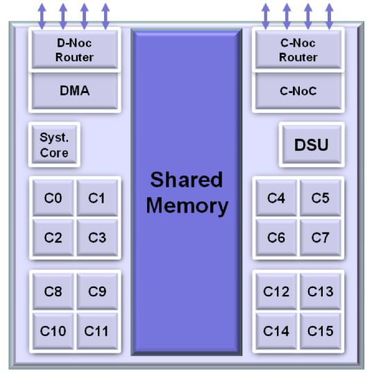
The MPPA-256 by Kalray is an array of 16 packet storage). The only timing effect that would
computing clusters and 4 specialized Input/Output not be observed with larger data is the time it takes
(IO) clusters connected by a NoC (Network on to compute the time-stamps themselves, but this can
Chip). The global architecture of the MPPA-256 is safely be neglected.
depicted in figure 5. Each square box corresponds The number of time-stamps that are necessary to
to a computing cluster. The four I/O clusters are perform useful measurements has to be confronted
represented on the four sides (east, west, north and to the cost of transmitting data on the network
south). Two of them are connected to a PCIe con- on chip. First, we choose the granularity, i.e., the
troller and the two others to an Ethernet controller. minimum packet size with which we associate time-
Each IO cluster has 4 cores. stamps to follow the route. The chosen granularity
A computing cluster is illustrated in figure 6. is set to one input sample processed by each core
It is composed of 16 computing cores (each core PE. To measure the MPPA latency, the latency of
is called a Processing Element or PE), one sys- the entire system (MPPA + host), and the computing
tem core (Resource Management), one NoC Rx duration on each worker, we need around 20 time-
(receiver) interface, one NoC Tx (transmitter) in- stamps. Each cluster has a Debug System Unit
terface, one DMA (Direct Memory Access) and (DSU) offering a 64-bit counter for time-stamping.
one DSU (Debug System Unit). They access con- We assume that our measures do not exceed 10
currently the 2MB shared memory. The overall seconds. For measuring up to 10s with the 2.5ns
architecture provides separate memory banks, and MPPA clock period, we need a 32-bit counter. With
reservation mechanisms on the NoC, which also all our experiments, the time-stamp overhead in the
contribute to predictability. data transmitted is estimated to be around 1%.8
B. Dimensioning Experiments 1.9
In [3], we show that the communication through 1.8
the IO cluster becomes the main bottleneck of the 1.7
system. We implement a pipeline architecture with 1.6
a double-buffer communication to parallelize the 1.5
communication and the internal cluster processing. 1.4
Another case study on the same platform described 0 50 100 150 200 250
in [4] had to address the same problem. Number of TDS1 revolutions
In order to observe the end-to-end latency, we
made an experiment where data is received by the Fig. 7: Evolution of indicator OM1 according to the
MPPA, and sent back to the host, without any number of revolutions of TDS1
computation.
The experiment is performed for increasing sizes
of data chunks, and 100 times for each size. The Online OM1 at step k is calculated by averaging all
MPPA latency remains less than 200 µs for sizes the k−1 previous shaft revolutions. OM1 converges
ranging from 4 to about 10000 bytes. from the 50th shaft revolution (k = 50) in Figure 7.
Since the size of one sample data is 4 bytes When k = 50, OM1 is equal to 1.84g . The relative
(a tuple made of a vibration measure and a phase error of OM1 computed in two different manner
sensor), we can choose any size lower (and close) to (on-ground versus on-board) is equal to 0.9%.
10000/4 = 2500 for the size of packets to be sent Comparing two OM1 values (on-ground and on-
by the HOST to the IO cluster. We actually choose board) does not make sense. People who analyze
VIBRATION CHUNK SIZE = 2048 = 8192/4 for the indicators results are not interested in absolute
the advantage of manipulating power-2 sized arrays. values of indicators but in the trend of indicators.
In other words, given the same set of samples, the
C. On-line HMS experiment results of indicators given by the two methods must
have the same trend.
Once chosen the data chunk size for transmission,
2) Comparison of on-ground and on-line OM1
we have set up an experiment to mimic the on-
indicator: In this experiment, we monitor the equip-
line computation of indicators. On the MPPA side,
ment input drive shaft left, whose rotational speed
we use 2 threads on the IO cluster core, ioreader
ratio is rt = 16.82 (it rotates 16.82 times faster than
and iowriter, and a Worker thread running on
the tail rotor). The purpose of this experiment is to
a computation core. The ioreader transmits the
compare the indicator OM1 in two cases. The first
vibration data coming from the host to the Worker
case corresponds to the OM1 indicator calculated
thread that computes the indicators, and iowriter
using the global algorithm (recall, a single value of
sends back indicators to the host.
OM1 is calculated after interpolating and averaging
On the host side, the host mimics the actual
all the monitored shaft revolutions). However, in
sensors by sending packets of vibration data stored
the case of the incremental algorithm, one OM1
in files. Those data were collected in real operation
is calculated at each monitored revolution by using
conditions from a servicing H 175 aircraft, and
a growing window. We compare the last value of
correspond to the acquisition of 224 monitored shaft
the incremental OM1 indicator and the OM1 com-
revolutions.
puted using the global algorithm. The experiment is
1) OM1 on-line indicator results: The OM1 in-
performed on 20 raw vibration files acquired during
dicator is computed as follows:
the same flight conditions. Figure 8 shows the OM1
indicator computed using different vibration files
2 × Module(FFT(AverageSignal))
with the global and incremental algorithms. We
where AverageSignal represents the average signal note that the error is tolerable in the case of OM1
of all 224 monitored shaft revolutions in the off-line indicator. For instance, the global and incremental
version of the application. The on-ground OM1 is OM1 computed at date1 are respectively equal to
equal to 1.823g . 3.013763g and 3.012429g . The two OM1 values
Unlike the on-ground version where only one are not exactly the same but the difference is very
OM1 is computed by using the average signal of small. Finally, the maximum relative difference af-
224 shaft revolutions, the on-board version com- ter computing OM1 indicator using 20 raw vibration
putes OM1 by using a growing window of samples. files is equal to 2.65%.9
3.2
+
+ ++
3 +
+ +
+ + +
2.8
+
+
2.6 +
+
+
+ +
2.4 +
+
2.2 +
global OM1 +
incremental OM1
2
date1 date5 date10 date15 date20
acquisitions date
Fig. 8: Comparison of on-ground and on-line OM1 indicator
10
9 +
8
7
6 +
+ +
5 +
+ +
+
4 + +
++ + +
+ ++ + + global RMSR +
+
3 incremental RMSR
date1 date5 date10 date15 date20
acquisitions date
Fig. 9: Comparison of on-ground and on-line RMSR indicator
3) Comparison of on-ground and on-line RMSR second step, harmonics specified in the V argument
indicator: The RMSR (Root Mean Square Resid- are removed. The third step consists in computing
ual) indicator is calculated as follows: the reverse FFT of the residual frequency spectrum.
4 Finally, the root mean square is calculated using the
residual temporal signal. This experiment has the
z }| {
3
same parameters as the previous one (same acqui-
z }| {
RM S(F F T −1 (Remove(F F T (AverageSignal), V )))
| {z } sition file and monitored shaft) and the purpose is to
1
| {z } compare the RMSR indicator calculated using the
2
global and the incremental algorithm. We replace
AverageSignal denotes the average of all moni- the global AverageSignal of the existing HMS by
tored shaft revolutions and V is the set of harmonics the average signal “until now”. Figure 9 shows that
to remove from the spectrum. The computation of the difference between the 2 versions is very small.
the RMSR indicator can be divided into four parts. The maximum difference is observed at date5 and
The first part consists in calculating the Fast Fourier equals to 4%.
Transform using the AverageSignal. During the10
VII. C ONCLUSION AND F UTURE W ORK which the HMS application can share the Kalray
with another application, raising questions about the
We have transformed an off-line on-ground com- criticality level of several applications sharing the
putation of health indicators, in which the global same platform.
average of a signal is used, into an on-line embed- We will also present the results of the new incre-
ded real-time computation of the same indicators, mental algorithms (not necessarily running on the
in which the average is done on a growing window. embedded platform) to the experts in charge of the
We used these experiments in order to validate the maintenance decisions. As mentioned previously,
error induced on the result of the computation, their decision should be the same. Some experts
and to provide dimensioning information for the have been already asked to look at the results, but
implementation of the full application. the complete procedure has not been conducted in
The lessons learnt are detailed below. First, any full for now.
globally computed value has to be transformed A longer-term prospect is to experiment with
into some feasible incremental version (the same machine learning techniques applied in the domain
function computed on either a sliding window, or a of predictive maintenance, and to explore the idea
growing window). There is no way to decide, based of implementing such a technique on the Kalray
on the algorithm alone, whether the discrepancies MPPA, to be connected to the computation of
produced are acceptable or not. The original de- the indicators. The coupling of these computations
signers of the signal processing algorithms have to would give an on-ground real-time surveillance and
be consulted, to assess the impact of this change on maintenance decision.
the results. The complete approach we followed can
be used as guidelines for the transformation of other R EFERENCES
signal processing applications, which are likely to
[1] B. de Dinechin, R. Ayrignac, P.-E. Beaucamps, P. Couvert,
exhibit the same kind of algorithms. B. Ganne, P. de Massas, F. Jacquet, S. Jones, N. Chaise-
For the future, if the idea of computing such martin, F. Riss, and T. Strudel. A clustered manycore
algorithms on an embedded platform is adopted, it processor architecture for embedded and accelerated ap-
plications. In High Performance Extreme Computing
means that the very first design of the algorithms Conference (HPEC), 2013 IEEE, pages 1–6, Sept 2013.
has to take this constraint into account: global [2] B. D. De Dinechin, D. Van Amstel, M. Poulhiès, and
averages, for instance, will be forbidden. G. Lager. Time-critical computing on a single-chip mas-
sively parallel processor. In Design, Automation and Test
Second, some tools on the execution platform in Europe Conference and Exhibition (DATE), 2014, pages
would really help. The host PC (which is used first, 1–6. IEEE, 2014.
before the actual acquisition card is connected to [3] M. Lo, N. Valot, F. Maraninchi, and P. Raymond. Imple-
the MPPA) could be real-time. It would allow more menting a real-time avionic application on a many-core
processor. In 42nd European Rotorcraft Forum, Lille,
precise estimations of the overall final behavior, France, sep 2016.
without the need for the acquisition card, in early [4] D. Madroñal, R. Lazcano, R. Salvador, H. Fabelo, S. Or-
stages of development. A precise timing tracing tool tega, G. Callico, E. Juarez, and C. Sanz. Svm-based
real-time hyperspectral image classifier on a manycore
is also needed (either with help from the hardware
architecture. Journal of Systems Architecture, 80:30–40,
for real executions, or with a cycle-accurate simu- 2017.
lator of the execution platform). We designed our [5] Mathworks. Predictive Maintenance with MATLAB; Avoid
own timestamps mechanism, knowing that, for the costly equipment failures by using sensor data analytics.
Mathworks, 2016.
application under study, intrusiveness is limited. But [6] J. Nowotsch, M. Paulitsch, D. Bühler, H. Theiling, S. We-
this should be studied again for another application, gener, and M. Schmidt. Multi-core interference-sensitive
which is not satisfactory. wcet analysis leveraging runtime resource capacity en-
forcement. In Real-Time Systems (ECRTS), 2014 26th
Further work will be done along several lines.
Euromicro Conference on, pages 109–118. IEEE, 2014.
First, we will finish the development and test of the [7] Sikorsky. Sikorsky, phi, metro demo real-time hums on
full HMS application on the Kalray MPPA, con- s-92. 3 2017.
nected to the real acquisition card; the full HMS in-
volves several sensors, takes input values at various
sampling frequencies, and takes into account several
distinct speed ratios with respect to the reference
shaft. Given the computing power of the MPPA,
it may work satisfactorily without optimizations.
The next step would be to develop solutions inYou can also read