The Wall: The Earth in True Natural Color from Real-Time Geostationary Satellite Imagery
←
→
Page content transcription
If your browser does not render page correctly, please read the page content below
remote sensing
Article
The Wall: The Earth in True Natural Color from
Real-Time Geostationary Satellite Imagery
Louis Gonzalez 1,∗         and Hirokazu Yamamoto 2
 1    LOA—Laboratoire d’Optique Atmosphérique, University of Lille, CNRS, UMR 8518, F-59000 Lille, France
 2    Geological Survey of Japan, National Institute of Advanced Industrial Science and Technology, 1-1-1-C7,
      Higashi, Tsukuba 305-8567, Japan; hirokazu.yamamoto@aist.go.jp
 *    Correspondence: louis.gonzalez@univ-lille.fr

 Received: 24 June 2020; Accepted: 20 July 2020; Published: 24 July 2020

 Abstract: We present “The Wall”, the first web-based platform that animates the Earth in true natural
 color and close to real-time. The living planet is displayed both during day and night with a pixel
 resolution of approximately 1 km and a time frequency of 10 min. The automatic processing chains
 use the synchronized measurements provided by three geostationary satellites: the METEOSAT
 Second Generation (MSG2), Himawari-8, and GOES-16. A Rayleigh scattering correction is applied,
 and a cloud of artificial neural networks, chosen to render “true natural color” RBG composites, is
 used to recreate the missing daytime bands in the visible spectrum. The reconstruction methodology
 is validated by means of the TERRA/AQUA “Moderate Resolution Imaging Spectroradiometer”
 (MODIS) instrument reflectance values. “The Wall” is a dynamic broadcasting platform from which
 the scientific community and the public can trace local and Earth-wide phenomena and assess their
 impact on the globe.

 Keywords: geostationnary satellites; MSG2 SEVIRI; Himawari-8 AHI; GOES-16; MODIS Terra/Aqua;
 true natural color imagery; atmospheric correction; artificial neural network

1. Introduction
      For many years geostationary satellites have surrounded and observed the Earth. In the last decade,
their resolution has improved to 1 km at nadir. At the same time, real-time reception of imagery has
become increasingly practical through satellite downlinks and online-accessible archives. However, little
effort has been devoted to the creation of images showing the whole Earth in the splendor of its natural
color. One of the main reasons is that often one or more components of the visible spectrum is not
measured by the sensors on-board the satellites. In this application, we have selected three geostationary
satellites to tile the entire globe: (1) The MSG2 “Spinning Enhanced Visible and Infrared Imager” (MSG2
SEVIRI) instrument managed by EUMETSAT was launched in 2002, and offers a resolution of 3 km at
nadir. It covers Europe, Africa, and the Middle East. However, the blue and green visible bands (0.4 and
0.5 µm) are missing and make this satellite almost blind over the spectral range of human vision. (2) The
NASA GOES-16 series “Advanced Baseline Imager” (ABI) [1] instrument covers the American continent.
Launched in 2016, and managed by NOAA, it has a resolution of 1 km at nadir but it lacks the visible
green band. (3) The Himawari-8 [2,3] “Advanced Himawari Imager” (AHI) instrument managed by the
Japan Meteorological Agency (JMA) was launched in 2014. This instrument captures all three visible
bands with a resolution of 1 km at nadir and covers the Western Pacific region. These three instruments
offer detailed and quantitative monitoring of a wide array of surface and atmospheric parameters [1,4].
Although the tracking of atmospheric and land-surface phenomena usually requires the interrogation
and combination of multiple spectral bands, we think it is also desirable for the human eye to view the
spectral data in natural color RGB composites to help the analysis of the image components.

Remote Sens. 2020, 12, 2375; doi:10.3390/rs12152375                        www.mdpi.com/journal/remotesensing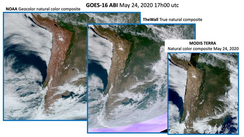
Remote Sens. 2020, 12, 2375 2 of 16
True color renderings of geostationary data can be assessed from the comparison with the orbiting
satellite imagers that hold three visible reflectance bands at approximately 0.4, 0.5 and 0.6 µm, hereafter
called RGB visible bands. In this work, we will use Moderate Resolution Imaging Spectroradiometer
(MODIS) as a reference.
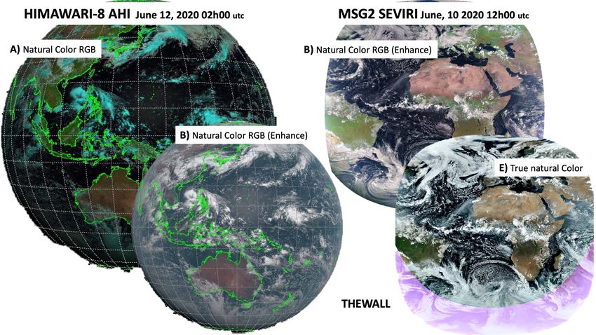
Today, several RGB composite terminologies are used: ”Natural color RGB”, ”Natural color RGB
(enhance)”, ”True color reproduction image”, and ”GeoColor”, as displayed in Figure 1, all trying to mimic
with more or less success what we think is ”True natural color” corresponding to the human vision.
Himawari-8 AHI uses the visible bands at 0.4697, 0.5094 and 0.6363 µm to directly build RGB images
called ”true color reproduction” images [3,5] (see inset (C) of Figure 1). Both Himawari-8 AHI and MSG2
SEVIRI create so-called ”natural color RGB” composites [6] (see inset (A) of Figure 1) using the bands
at 1.6, 0.8 and 0.6 µm, in which the clouds appear blue-green. Alternatively, the clouds are replaced
by white levels, leading to the ”natural color RGB (Enhance)” composite (see inset (B) of Figure 1).
The best RGB rendering is the ”GeoColor” approach for GEOS-16 (see inset (D) of Figure 1), for which
the missing green band is reconstructed either from correlations to adjacent bands or from a lookup
table constructed from Himawari-8 AHI green band [7,8].
The project is named “The Wall” as a huge billboard broadcasting over the globe the best possible
color rendering of geostationary satellite images and animations to the public and to the scientific
community. It is thus necessary to create ”true natural color” images for the three complementary
satellites (GOES-16 ABI, MSG2 SEVIRI, and Himawari-8 AHI), using visible bands which, in cases
where they are lacking on sensors like MSG2 SEVIRI and GOES-16 ABI, have to be reconstructed.
In the published NASCube (North African Sandstorm Survey) project and web platform [9], we have
demonstrated that artificial neural networks (ANNs) are very powerful to reconstruct reflectance
signals of the MSG2 SEVIRI instrument. ANNs were also used to track sandstorms over the Sahara
and Middle East and to estimate their optical thicknesses. We propose hereafter to apply this ANN
methodology to predict the missing green band for the GOES-16 ABI. The reconstruction will be
validated by comparison with the NASA MODIS products.
Figure 1. Cont.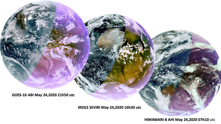
Remote Sens. 2020, 12, 2375                                                                                  3 of 16

      Figure 1. Illustrations of existing color renderings labeled as (A) natural color RGB, (B) natural color
      RGB (Enhance), and (C) True color reproduction image created for Himawari-8 AHI. (D) GeoColor created
      for GOES-16 ABI; (E) true natural color RGB composites from this work for “The Wall” application
      (Himawari-8 AHI, MSG2 SEVIRI and GOES-16 ABI).

2. Methodology to Process the Geostationary Satellite Data
     The aim of the study is to present a homogeneous visualization of the main atmospheric and terrestrial
phenomena during day and night times, using data acquired simultaneously from three instruments with
measurement characteristics that differ in terms of wavelengths, pixel sizes, and acquisition time delays.
To perform this task, we have collected the level 1B data products, and calibrated and geolocated radiances
expressed in radiance units W sr−1 m−2 over the Full Disk (FD).
     We first present the specifications of the spectral bands used for each satellite (see Section 2.1).
Section 2.2 explains the construction of the pseudocolor composites in night-time from several thermal
infrared bands. Section 2.3 details the atmospheric corrections applied to the used spectral visible
and near-infrared (NIR) bands. It also focuses on the key algorithms designed and implemented to
reconstruct the missing visible bands for GOES-16 ABI and MSG2 SEVIRI, and finally build ”true
natural color” composite images.

2.1. Spectral Bands and Satellite Specifications of the Level 1B Data Products

2.1.1. Satellites with 1 km Resolution at Nadir
     Both Himawari-8 AHI and GOES-16 ABI have a 1 km resolution at nadir and an acquisition
delay time of 10 min. Himawari-8 AHI monitors the West Pacific ((144.418°W, 64.903°E)/(75.348°S,
75.348°N)). It is managed by the Japan Meteorological Agency (JMA) with on the on-board instrument
AHI imager. The data is distributed by the National Institute of Information and Communications
Technology (NICT) Science Cloud [10,11]. We have processed 6 of the 16 available bands, referenced
by their central wavelength: 0.4697, 0.5094, 0.6363, 3.8823, 8.5878, and 9.6329 µm. The first three map
the visible range as displayed in Figure 2.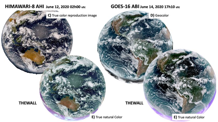
Remote Sens. 2020, 12, 2375                                                                                    4 of 16

   1.0

                                                                     HIMAWARI-8 AHI
  0.0

  0.0        ?                                                           GOES-16 ABI

  0.0       ??                                                           MSG2 SEVIRI

  0.0                                                                    MODIS
    0.40             0.60           0.80           1.00           1.20           1.40          1.60           1.80
                                                          λ[µm]

        Figure 2. Normalized spectral response functions of Himawari-8 AHI, GOES-16 ABI, MSG2 SEVIRI
        (solid lines), and MODIS (dotted lines) visible and near-infrared (VNIR) bands, shifted along the y-axis
        for the sake of clarity. The questions marks indicate the missing visible bands in GOES-16 ABI and
        MSG2 SEVIRI imagers.

     To map the American continent, we have used the GOES-16 ABI-EAST region ((156.299°W, 6.299°E)/
(81.328°S, 81.328°N)) which is managed by the National Environmental Satellite, Data, and Information
Service (NESDIS) with the on-board ABI and distributed by the Google Cloud Platform [12]. We have
processed 6 of the 16 bands, referenced by their central wavelengths: 0.4702, 0.6365, 0.8639, 3.8905, 8.4444
and 9.6072 µm. Note that the green visible band is missing in this instrument.

2.1.2. MSG2 SEVIRI Data with 3 km Resolution at Nadir
     The MSG2 geostationary platform, equipped with MSG2 SEVIRI instrument, provides observations
of Europe, Africa, Middle East, etc. ((81.236°W, 81.236°E)/(81.144°S, 81.144°N)), every 15 min since
2004. The satellite is managed by the European Organization for the Exploitation of Meteorological
Satellites (EUMETSAT). We have processed 6 out of the 12 distributed spectral channels, referenced by
their central wavelengths: 0.6, 0.8, 1.6, 3.9, 8.7 and 9.7 µm. Note that both the blue and green visible
bands are missing as indicated in Figure 2.

2.2. Night-Time RGB Composite
     The RGB rendering of night-time images is not straightforward. One option is to render them in
gray levels. In “The Wall”, we currently offer two empirical algorithms designed with the primary aim
of keeping a visual day/night white color transition of the clouds for the NIR bands shown in Figure 3.
The final night composite is sufficiently sensitive to show in the video animations the propagation of the
thermal changes over the Earth surface. The first algorithm is taken from that used for the NASCube
project [9] and is directly applied to GOES-16 ABI. The second algorithm is a linear combination of
bands applied to Himawari-8 AHI images. The results are close enough to offer a smooth visualization
over the whole globe.
     The three MSG2 SEVIRI (3.9, 8.7 and 9.7 µm) and GOES-16 ABI (3.8905, 8.4444 and 9.6072 µm) radiances
are used to build the RGB (0; 255) Pseudo-Night Composites (PNC) for each instrument acquisition. The final
image is directly computed by means of a linear-log transformation of the corresponding radiance values ρi :

                                                    log (10000 × ( ai − bi ρi )) − mini
                              PNC (λi ) = 256 ×                                         .                            (1)
                                                             (maxi − mini )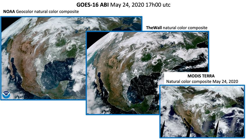
Remote Sens. 2020, 12, 2375                                                                                5 of 16

     For Himawari-8 AHI, the RGB PNC is constructed from the following three bands (3.8823, 8.5878
and 9.6329 µm), and the final image is computed using a linear transformation of the corresponding
radiance values:

                                         PNC (λi ) = 256 × ( ai − bi ρi )                                      (2)

     The ai , bi , mini , and maxi parameters are listed in Table 1. They were empirically adjusted to yield
the best contrast for the resulting night images, as illustrated in Figure 4. Figures 5 and 6 illustrate
the ability of the night composite to highlight the ground hot spots. In Figure 5, the active bushfires
that raged in early 2020 in Australia are visible as dark spots on the night RGB image. In Figure 6,
the activity of the Klyuchevskaya volcano in the Kamchatka Peninsula appears as a blue hot spot.

      1.0

                                                   HIMAWARI-8 AHI
     0.0

                                                   GOES-16 ABI
     0.0

                                                   MSG2 SEVIRI
     0.0
       3.00            4.00       5.00          6.00              7.00        8.00           9.00      10.00
                                                        λ[µm]

      Figure 3. Normalized spectral response functions of Himawari-8 AHI, GOES-16 ABI, and MSG2
      SEVIRI infrared bands in µm, shifted along the y-axis for the sake of clarity. These bands are used to
      build the Pseudo-Night Composites.

      Table 1. Parameters for the linear-log and linear transformations to the Pseudo Night Composites for
      MSG2 SEVIRI, GOES-16 ABI, and Himawari-8 AHI satellites.

                    λi (µm)   PNC Channel              ai                bi          mini    maxi
                              MSG2 SEVIRI
                    3.88      R                        0.004975          1.308458    7.5         9.5
                    8.58      G                        0.002165          1.246753    7.7         9.5
                    9.63      B                        0.004202          1.899160    7.5         9.5
                              GOES-16 ABI
                    3.89      R                        0.000338          1.007768    7.5         9.5
                    8.44      G                        0.000501          1.046115    7.7         9.5
                    9.60      B                        0.001000          1.176000    7.5         9.5
                              Himawari-8 AHI
                    3.9       R                    −1.269036             0.842010          N/A
                    8.7       G                    −0.119018             1.118907          N/A
                    9.7       B                    −0.181937             1.250030          N/A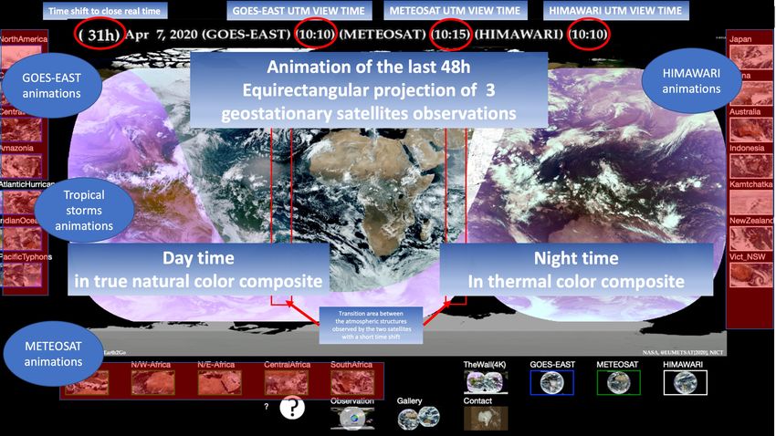
Remote Sens. 2020, 12, 2375                                                                                     6 of 16

      Figure 4. Examples of day and night RGB composites for GOES-16 ABI (left), MSG2 SEVIRI (middle),
      and Himawari-8 AHI (right) data for the same day 24 May 2020.

      Figure 5. Day and night views of the January 2020 bushfires raging on Victoria region’s eastern coast in
      Australia, which were captured by Himawari-8 AHI. The fire activity is visible at night as dark/blue spots.

      Figure 6. Night views of the active Klyuchevskaya volcano in the Kamchatka Peninsula in May 2020,
      captured by Himawari-8 AHI.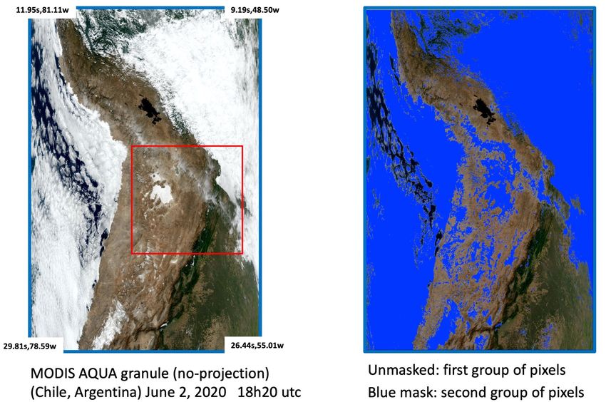
Remote Sens. 2020, 12, 2375                                                                             7 of 16

2.3. Daytime RGB Composite
     Daytime reflectance values are rendered with a ”True Natural Color RGB Composite” (TNCC) that
is built from visible reflectance data. For MSG2 SEVIRI and GOES-16 ABI, we had to reconstruct the
missing visible bands with a cloud of ANNs, which is applied to the spectral bands that have been
corrected for atmospheric effects as described below.

2.3.1. Atmospheric Corrections
     To obtain natural colors from the recorded reflectance values, the minimum atmospheric correction
required is the compensation for the Rayleigh scattering contribution, to which a correction for ozone
aerosols was added according to the 6S radiative transfer code (6sV2.1) [13]. The corrections are
identical to that applied for the NASCube study [9], but we list them here for the sake of completeness.
Let Lm (W sr−1 m−2 ) be the Top-Of-Atmosphere (TOA) radiance in band m and ρm the TOA reflectance,
calculated as

                                              ρm = πLm /µs Es ,                                            (3)

with µs = cos θs , where θs is the solar zenith angle, and with Es the solar flux at the top of the
atmosphere. The Rayleigh and ozone corrections assuming a Lambert’s law of the surface reflectance
defines ρm as

                                                     T (µs ) T (µv )ρs

                                    ρm = TO3 ρ atm +                     ,                                 (4)
                                                      1 − ρs · Salb

where ρS stands for the surface reflectance, Salb is the spherical albedo of the atmosphere, and µv = cos θv ,
with θv the view zenith angle as defined in the 6S reference manual [14,15]. In Equation (4), TO3 accounts
for the light absorption on the direct downward and upward paths through the stratospheric ozone layer:

                                                                1        1
                              TO3 = exp − AO3 · µO3 ·                +               ,                     (5)
                                                              cos θs   cos θv

where µO3 is the ozone absorber amount for each satellite wavelength, and AO3 is the ozone absorption
coefficient by Shettle et al. [16], tabulated in steps of 200 cm−1 between 13.000 and 24.200 cm−1 and by
steps of 500 cm−1 between 27.500 and 50.000 cm−1 .
     The other terms of Equation (4) correspond to atmospheric effects and are estimated assuming both
a black surface and a pure molecular atmosphere. ρ atm is the atmospheric reflectance that corresponds
to the light directly scattered by the atmosphere. It is computed by the analytical expressions [14]
that reproduce Chandrasekhar isotropic scattering values [17]. T (µs ) and T (µv ) are the transmission
fluxes of the atmosphere on the path between the sun and the surface, and, respectively, between the
surface and the sensor. Both are estimated from the Delta–Eddington approximation [18], such as

                                             (2/3 + µ) + (2/3 − µ) · e−τ/µ
                                   T (µ) =                                 ,                               (6)
                                                       (4/3 + τ )

where µ is the cosine of the solar and/or observational zenith angle and τ is the optical thickness.
For a pure molecular atmosphere and for some observation conditions (µs , µv , and ρS ), numerical
figures of ρm were derived directly (independently) from the “successive orders of scattering” code
of Lenoble et al. [19]. By reporting these contributions to the left-hand side of Equation (4), Salb
can be derived, leading to Salb = 0.0497, 0.0198, and 0.0012 for wavelengths 0.615, 0.810 and 1.64 µm,
respectively. Assuming that (ρs · Salb )  1 in Equation (4), the surface reflectance can be computed as

                                                   (ρm/TO3 − ρ atm )
                                           ρ∗s =                     ,                                     (7)
                                                    T (µs ) T (µv )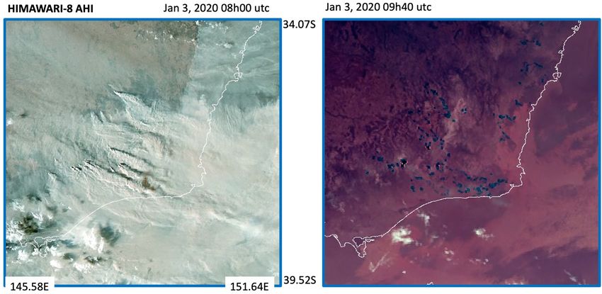
Remote Sens. 2020, 12, 2375                                                                         8 of 16

from where, the surface reflectance is computed as

                                                          ρ∗s
                                             ρs =                   .                                  (8)
                                                     1 + Salb · ρ∗s

2.3.2. RGB Visible Composites
    Once all three visible bands are fetched or reconstructed, the daytime RGB composite TNCC can
be built by log-transforming the 0.4, 0.5 and 0.6 µm (0; 255) RGB visible bands colors:

                                                   log (10000 × ( ai − bi ρi )) − mini
                              TNCC (λi ) = 256 ×                                       ,               (9)
                                                            (maxi − mini )

with mini and maxi values in the range of 5.8 to 9.6, respectively.

2.3.3. Reconstruction of the Missing Green Band for GOES-16 ABI
     The details of the ANN methodology used to reconstruct the missing blue and green bands (0.4
and 0.5 µm) of the MSG2 SEVIRI sensors are given in Ref. [9]. The use of an ANN is clearly superior to
any lookup table, or other band correlation algorithm, as our true natural color composites for MSG2
SEVIRI images appear more natural than the MSG Natural Color RGB (Enhance)-distributed product
(see Figure 1), the reference being MODIS imagery as discussed later in the paper.
     Fine-tuning the parameters of an ANN (Stuttgart Neural Network Simulator (SNNS) [20]) to
faithfully reconstruct GOES-16 ABI green reflectances turned out to be a tricky process. We have
designed an ANN that takes as training inputs the three MODIS 0.469, 0.645 and 0.858 µm (spectrally
close to the GOES-16 ABI bands, 0.47, 0.636 and 0.863 µm, as seen from Figure 2), and the green MODIS
band at 0.555 µm as target values. This ANN is a fully connected feedforward network [21]. The ANN
topology we present yields the best green retrieval out of many tests we carried out. It consists of two
hidden layers with 8 nodes each (See Figure 7). The training data set is composed of a selection of
about thirty MODIS granules for which we hand-selected representative areas such as water, ocean
colors, deserts, rocks, white and bright surfaces, etc. Once trained, the network was tested on various
MODIS granules and the training ANN data set was enlarged with those showing inaccurate—poor
correlation with respect to MODIS real green reflectances—reconstructed green values.
     From our recent experience with the design of ANNs for aerosol optical depth retrievals and with
the reconstruction of the lacking ASTER blue band [9,22], we have demonstrated that the training and
accuracy of ANNs are improved if applied to specific classes of reflectance values. Thus, our new
algorithm uses MODIS values that are classified according to the empirically chosen values x defining
two main groups:
                                    2
              x = ρ MODIS (0.469) + (ρ MODIS (0.469) + ρ MODIS (0.645) + ρ MODIS (0.858)) ,          (10)
                                    3
the first one corresponding to water, dark areas, and vegetation (x < 0.2), and the second one to desert
or cloudy areas (x > 0.2). Figure 8 is an example of the pixel classification over one MODIS granule,
the first group being the unmasked pixels and the second group appearing in blue.
      The histograms of the two groups of all MODIS input values are shown in Figure 9. Each of the two
histograms is split to generate subclasses of pixel values defining the inputs of ANNs. The determination
of the number of data by classes (bins) was carried out in stages by monitoring both the convergence
of the networks and the quality of the green retrieval over the MODIS granules composing the training
data sets. It soon became clear that the first group requires 1536 networks and converges with an average
number of 6000 pixels per bin and the second group requires 1256 networks and converges with an
average number of 3000 pixels per bin. For each bin of the histograms of Figure 9, a dedicated ANN
with the architecture defined before (3 inputs, 2 hidden layers with 8 nodes each, and 1 output value, see
Figure 7), is designed. Altogether, an ensemble of 2792 ANNs is trained.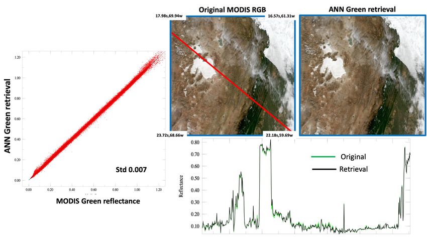
Remote Sens. 2020, 12, 2375                                                                                 9 of 16

                              Input          Hidden             Hidden             Output
                              layer           layer              layer              layer

          ρ(0.469 µm)

          ρ(0.645 µm)
                                                                                              ρ(0.555 µm)
          ρ(0.858 µm)

      Figure 7. Topology of the artificial neural network (ANN) with one input layer taking 0.469, 0.645 and
      0.858 µm as the reflectance values and 0.555 µm as the target value.

      Figure 8. Illustration of the pixel classification of the training Moderate Resolution Imaging
      Spectroradiometer (MODIS) data. Unmasked pixels enter the first group (x < 0.2), while the second
      group (x > 0.2) is marked in blue. The red-selected area is used for subsequent correlation plots shown
      in Figures 10 and 11.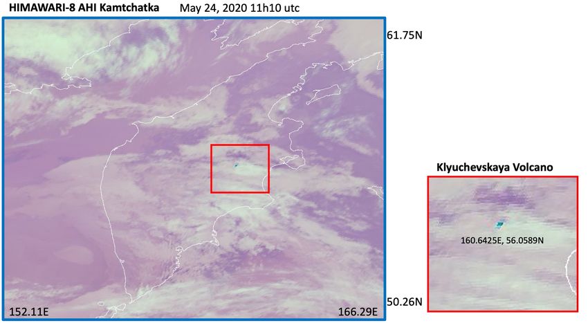
Remote Sens. 2020, 12, 2375                                                                                                                                                  10 of 16

                                                                                                                0.47
             0.20
                                                                 Bin width: 0.000156                            0.42                                   Bin width: 0.001433
             0.18
                                                                                                                0.37
             0.16
                                                                                                                0.32
             0.14

                                                                                                     Pixels %
                                                                                                                0.27
  Pixels %

             0.12
                                                                                                                0.22
             0.10
                                                                                                                0.17
             0.08
                                                                                                                0.12
             0.06
                                                                                                                0.07
             0.04
                                                                                                                0.02
             0.02
                0.00   0.02   0.04   0.06   0.08   0.10   0.12   0.14      0.16        0.18   0.20                 0.20     0.40    0.60    0.80    1.00            1.20          1.40

                        (a) Histogram for x < 0.2 values.                                                                 (b) Histogram for x > 0.2 values.
  Figure 9. Histograms of the two x-value groups (Equation (10)) of MODIS data to define the ANNs’ inputs.

             Figure 10. Illustration of the green reconstruction over the South American red-selected area in Figure 8.
             The left image is a RGB MODIS granule; the right image is the same but using the ANN reconstructed
             green band. The green and black curves represent the green reflectances across the red marked transects,
             for the original and reconstructed images, respectively.

             Figure 11. Correlation plots between the GOES-16 ABI and MODIS red, green, and blue reflectance
             values for two reprojected images over the same region in South America marked in red in Figure 8.
             The GOES-16 ABI and MODIS images are taken within few minutes. The “GOES-16 Ret” green
             reflectance values were predicted by the cloud of ANNs.
Remote Sens. 2020, 12, 2375 11 of 16
3. Results and Discussion
3.1. Validation of the ANN Green Reconstruction for GOES-16
To assess the quality of the ANN green reconstruction for GOES-16, we have considered a MODIS
granule far away in time from the ANN training data set shown in Figure 8, and we focus on the
red-selected area. The correlation plot drawn on the left-hand side of Figure 10 shows the excellent
correlation between the native MODIS green reflectance values and the ones predicted by the cloud
of ANNs over the full granule. To further illustrate the accuracy of the green reconstruction, we also
present, on the same figure, the plots of the green reflectance values over the red transect. The green
(original) and black (ANNs retrieval) curves are in nearly perfect agreement, illustrating that the 1 km
MODIS resolution is preserved.
In Figure 11, we have drawn the correlation plots between the GOES-16 ABI and MODIS red,
green, and blue reflectance values for two reprojected images over the same region of South America
(Chile/Argentina) taken within few minutes. As the images do not perfectly spatially overlap, we note
some spreading in the correlations for the red and blue bands that directly mirror into the spreading of
the correlation of the green reflectance values. In conclusion, both Figures 10 and 11 fully validate the
ANN-based green reconstruction methodology for GOES-16 ABI.
Figures 12 and 13 allow to compare the same scenes, in natural color components, as rendered
by MODIS, GOES-16 ABI with our ANN reconstructed green channel, and with the GeoColor
RGB composite. As MODIS has three visible wavelengths, it must approach the reality. These
figures convincingly illustrate that our RGB composite faithfully reproduces the MODIS RGB colors.
The matching is nearly perfect over rocks and desert areas, while we may pinpoint differences
over vegetated areas, due to the lack of Bidirectional Reflectance Distribution Function (BRDF)
correction effects.
Figure 12. Comparison of our GOES-16 true natural color RGB composite to the GeoColor natural color
composite and MODIS data, all taken over South America on 24 May 2020.Remote Sens. 2020, 12, 2375 12 of 16
Figure 13. Comparison of our GOES-16 true natural color RGB composite to the GeoColor natural color
composite and MODIS data, all taken over North America on 24 May 2020.
3.2. Description of ”The Wall” Processing Chain and Web Visualization Platform
Table 2 lists the current web-based platforms that present imagery of the MSG2 SEVIRI,
Himawari-8, and GOES-16 geostationary satellites. “The Wall” is the first platform to present
synchronized views of these three satellites. It acquires the data of the three geostationary satellites as
they are made available on the distribution platforms. The Level1B data are processed according to the
flowchart in Figure 14 within a few minutes to generate all the animated global mosaics and subsets.
The acquisition step uses simultaneously on three Linux-based computing nodes with 24 cores each,
while the data processing is carried out on a computing node with 32 cores and 96 GB of RAM. “The
Wall” web platform (http://earth2day.com/TheWall) homepage presents a global animation of the
Earth in plate-Carree projection, in which the views of the three satellites are alive, as illustrated by the
snapshot in Figure 15. The central panel is surrounded by focuses on specific Earth regions. In addition,
a gallery (see Table 3) shows exceptional events and will be updated periodically. “The Wall” gives
quick access to various areas of the globe, where the user can admire the dancing clouds over the
equatorial regions, measure the strength of frequent immense desert sandstorms, the extent of the
large forest fires, and the path of tropical storms. Being able to see the Earth alive on a wall gives us all
a vision of both its finite size and its fragility.Remote Sens. 2020, 12, 2375 13 of 16
Figure 14. “The Wall” flowchart. “The Wall” system is divided in three levels. The first level is devoted
to the data acquisition from the three geostationary satellites (EUMETCAST distribution, Google Cloud
Platform, and the NICT Science Cloud [10,11]). The second level computes the RGB true natural color
composites. The third one creates all the animated global mosaics and subsets.
Figure 15. Snapshot of “The Wall” website at http://earth2day.com/TheWall.Remote Sens. 2020, 12, 2375 14 of 16
Table 2. An incomplete list of web-based platforms for geostationary satellite imagery.
GOES-16 satellite
GOES-16 imagery
https://www.goes-r.gov/multimedia/dataAndImageryImagesGoes-16.html#GOES-EastOperational
NOAA GOES image viewer
https://www.star.nesdis.noaa.gov/GOES/fulldisk.php?sat=G17
GOES-16 and Himawari-8 satellites
SSEC Geostationary Satellite Imagery
https://www.ssec.wisc.edu/data/geo/#/animation
Himawari-8 satellite
NICT
https://himawari8.nict.go.jp/
JAXA EORC
https://www.eorc.jaxa.jp/ptree/index.html
Meteorological Satellite Center of JMA
https://www.data.jma.go.jp/mscweb/data/himawari/index.html
MSG2 SEVIRI
ICARE
https://www.icare.univ-lille.fr/data-access/browse-images/geostationary-satellites/
METEOSAT
http://www.meteo-spatiale.fr/src/images_en_direct.php
NASCube
http://nascube.univ-lille1.fr/
Table 3. List of events presented in “The Wall” gallery.
Events and hyperlinks to
http://earth2day.com/TheWall/Gallery/gallery.html
A huge sandstorm crossing the Atlantic in June 2020
http://earth2day.com/TheWall/Gallery/Movies/SANDSTORM20200611140020200620160016F.html
Huge fires in Canada in June 2019
http://earth2day.com/TheWall/Gallery/Movies/NORTHAMERIC2201905280000201906032355.html
One km accuracy image showing multiple fires in Amazonia in August 2019
http://earth2day.com/TheWall/Gallery/Movies/AMAZONI1km201908110000201908172300.html
Wild fires in the South East of Australia in January 2020
http://earth2day.com/TheWall/Gallery/Movies/VICT_OSW202001010000202001080700.html
Huge sand storm covering Australia in January 2020
http://earth2day.com/TheWall/Gallery/Movies/AUSTRALI2202001100600202001130600.html
Huge sand storm starting in Mongolia and crossing China toward Japan in May 2020
http://earth2day.com/TheWall/Gallery/Movies/MONGOLIASANDSTORM202005110600202005130540.html
4. Conclusions and Perspectives, and “The Wall” Website
“The Wall” is the first attempt to provide an operational platform to visualize in nearly real-time
all the atmospheric events occurring on our planet (±70.0°). The platform can be easily tuned to the
needs of the user and can be extended to include additional algorithms, such as BRDF corrections.
The ANN-based reconstruction of the missing visible bands can be implemented in a straightforward
manner to postprocess any image from the geostationary archives. The system has been running for
several months with minimal human maintenance. We are eagerly waiting for the launch of the next
generation of METEOSAT (MTG-I) by the end of 2021, which has an onboard "Flexible Combined
Imager (FCI)” instrument. This will make “The Wall” homogeneous in spatial resolution and will
allow a complete synchronization of its animations.Remote Sens. 2020, 12, 2375 15 of 16
Author Contributions: Conceptualization, methodology, software, and validation, L.G.; resources, L.G. and
H.Y.; writing—review and editing, L.G. and H.Y. All authors have read and agreed to the published version of
the manuscript.
Funding: This research received no external funding.
Acknowledgments: All MODIS products are courtesy of the online Data Pool at the NASA Land Processes
Distributed Active Archive Center (LP DAAC), USGS/Earth Resources Observation and Science (EROS) Center,
Sioux Falls, South Dakota. We wish to thank Eumetsat and Eumetcast for providing access to the MSG2 SEVIRI
instrument measurements. Himawari-8 AHI data is obtained from NICT Science Cloud Himawari Satellite Project
operated by the National Institute of Information and Communications Technology (NICT).
Conflicts of Interest: The authors declare no conflicts of interest.
Abbreviations
The following abbreviations are used in this manuscript.
ABI Advanced Baseline Imager
AHI Advanced Himawari Imager
MODIS Moderate Resolution Imaging Spectroradiometer
MSG2 SEVIRI Meteosat Second Generation Spinning Enhanced Visible and Infrared Imager
NICT National Institute of Information and Communications Technology
PNC Pseudo Night Composite
TNCC True Natural Color Composite
References
1. Schmit, T.J.; Griffith, P.; Gunshor, M.M.; Daniels, J.M.; Goodman, S.J.; Lebair, W.J. A Closer Look at the ABI
on the GOES-R Series. Bull. Am. Meteorol. Soc. 2017, 98, 681–698. [CrossRef]
2. Bessho, K.; Date, K.; Hayashi, M.; Ikeda, A.; Imai, T.; Inque, H.; Kumagai, Y.; Miyakawa, T.; Murata, H.;
Ohno, T.; et al. An Introduction to Himawari-8/9—Japan’s New-Generation Geostationary Meteorological
Satellites. J. Meteorol. Soc. Jpn. Ser. II 2016, 94, 151–183. [CrossRef]
3. Murata, H.; Saitoh, K.; Sumida, Y. True Color Imagery Rendering for Himawari-8 with a Color Reproduction
Approach Based on the CIE XYZ Color System. J. Meteorol. Soc. Jpn. Ser. II 2018, 96B, 211–238. [CrossRef]
4. Schmit, T.J.; Lindstrom, S.S.; Gerth, J.J.; Gunshor, M.M. Applications of the 16 Spectral Bands on the
Advanced Baseline Imager (ABI). J. Oper. Meteorol. 2018, 6, 34–46. [CrossRef]
5. Himawari Real-Time Image. Available online: https://www.data.jma.go.jp/mscweb/data/himawari/sat_
img.php (accessed on 13 June 2020).
6. Natural Colour Enhanced RGB—MSG—0 Degree. Available online: https://navigator.eumetsat.int/
product/EO:EUM:DAT:MSG:NCL_ENH (accessed on 13 June 2020).
7. Miller, S.D.; Schmidt, C.C.; Schmit, T.J.; Hillger, D.W. A case for natural colour imagery from geostationary
satellites, and an approximation for the GOES-R ABI. Int. J. Remote Sens. 2012, 33, 3999–4028. [CrossRef]
8. Miller, S.D.; Lindsey, D.T.; Seaman, C.J.; Solbrig, J.E. GeoColor: A Blending Technique for Satellite Imagery.
J. Atmos. Ocean. Technol. 2020, 37, 429–448. [CrossRef]
9. Gonzalez, L.; Briottet, X. North Africa and Saudi Arabia Day/Night Sandstorm Survey (NASCube).
Remote Sens. 2017, 9, 896. [CrossRef]
10. Murata, K.T.; Pavarangkoon, P.; Higuchi, A.; Toyoshima, K.; Yamamoto, K.; Muranaga, K.; Nagaya, Y.;
Izumikawa, Y.; Kimura, E.; Mizuhara, T. A web-based real-time and full-resolution data visualization for
Himawari-8 satellite sensed images. Earth Sci. Inform. 2018, 11, 217–237. [CrossRef]
11. Murata, K.T.; Watanabe, H.; Ukawa, K.; Muranaga, K.; Suzuki, Y.; Yamamoto, K.; Kimura, E. A Report of the
NICT Science Cloud in 2013. J. Jpn. Soc. Inf. Knowl. 2014, 24, 275–290.
12. Google Cloud Platform for GOES-16 ABI. Available online: https://console.cloud.google.com/marketplace/
product/noaa-public/goes-16?pli=1 (accessed on 13 June 2020).
13. Vermote, E.F.; Kotchenova, S.Y.; Tanré, D.; Deuzé, J.L.; Herman, M.; Roger, J.C.; Morcrette, J.J. 6SV Code.
2015. Available online: http://6s.ltdri.org/2015 (accessed on 13 June 2020).
14. Vermote, E.; Tanré, D. Analytical expressions for radiative properties of planar Rayleigh scattering media,
including polarization contributions. J. Quant. Spectrosc. Radiat. Transf. 1992, 47, 305–314. [CrossRef]Remote Sens. 2020, 12, 2375 16 of 16
15. Vermote, E.F.; Tanré, D.; Deuzé, J.L.; Herman, M.; Morcrette, J.-J. Second Simulation of the Satellite Signal in
the Solar Spectrum, 6S: An overview. IEEE Trans. Geosci. Remote Sens. 1997, 35, 675–686. [CrossRef]
16. Shettle, E.P.; Kneizys, F.X.; Gallery, W.O. Suggested modification to the total volume molecular scattering
coefficient in lowtran: Comment. Appl. Opt. 1980, 19, 2873–2874. [CrossRef]
17. Chandrasekhar, S. Radiative Transfer; Dover Publications, Inc.: New York, NY, USA, 1960.
18. Joseph, J.H.; Wiscombe, W.J.; Weinman, J.A. The Delta-Eddington Approximation for Radiative Flux Transfer.
J. Atmos. Sci. 1976, 33, 2452–2459. [CrossRef]
19. Lenoble, J.; Herman, M.; Deuzé, J.L.; Lafrance, B.; Santer, R.; Tanré, D. A successive order of scattering code
for solving the vector equation of transfer in the earth’s atmosphere with aerosols. J. Quant. Spectrosc. Radiat.
Transf. 2007, 107, 479–507. [CrossRef]
20. Zell, A.; Mache, N.; Hübner, R.; Mamier, G.; Vogt, M.; Schmalzl, M.; Herrmann, K.U. SNNS (Stuttgart
Neural Network Simulator). In Neural Network Simulation Environments; Springer: Boston, MA, USA, 1994;
pp. 165–186.
21. Miikkulainen, R. Topology of a Neural Network. In Encyclopedia of Machine Learning; Sammut, C., Webb, G.I.,
Eds.; Springer US: Boston, MA, USA, 2010; pp. 988–989. [CrossRef]
22. Gonzalez, L.; Vallet, V.; Yamamoto, H. Global 15-Meter Mosaic Derived from Simulated True-Color ASTER
Imagery. Remote Sens. 2019, 11, 441. [CrossRef]
© 2020 by the authors. Licensee MDPI, Basel, Switzerland. This article is an open access
article distributed under the terms and conditions of the Creative Commons Attribution
(CC BY) license (http://creativecommons.org/licenses/by/4.0/).You can also read