2D Analytical Model for the Directivity Prediction of Ultrasonic Contact Type Transducers in the Generation of Guided Waves - KTU ePubl
←
→
Page content transcription
If your browser does not render page correctly, please read the page content below
sensors
Article
2D Analytical Model for the Directivity Prediction
of Ultrasonic Contact Type Transducers
in the Generation of Guided Waves
Kumar Anubhav Tiwari *            ID
                                       , Renaldas Raisutis, Liudas Mazeika and Vykintas Samaitis
 Prof. K. Barsauskas Ultrasound Research Institute, Kaunas University of Technology, K. Baršausko St. 59,
 LT-51423 Kaunas, Lithuania; renaldas.raisutis@ktu.lt (R.R.); liudas.mazeika@ktu.lt (L.M.);
 vykintas.samaitis@ktu.lt (V.S.)
 * Correspondence: k.tiwari@ktu.lt; Tel.: +370-6469-4913

 Received: 22 February 2018; Accepted: 24 March 2018; Published: 26 March 2018

 Abstract: In this paper, a novel 2D analytical model based on the Huygens’s principle of wave
 propagation is proposed in order to predict the directivity patterns of contact type ultrasonic
 transducers in the generation of guided waves (GWs). The developed model is able to estimate the
 directivity patterns at any distance, at any excitation frequency and for any configuration and shape
 of the transducers with prior information of phase dispersive characteristics of the guided wave
 modes and the behavior of transducer. This, in turn, facilitates to choose the appropriate transducer
 or arrays of transducers, suitable guided wave modes and excitation frequency for the nondestructive
 testing (NDT) and structural health monitoring (SHM) applications. The model is demonstrated for
 P1-type macro-fiber composite (MFC) transducer glued on a 2 mm thick aluminum (Al) alloy plate.
 The directivity patterns of MFC transducer in the generation of fundamental guided Lamb modes
 (the S0 and A0) and shear horizontal mode (the SH0) are successfully obtained at 80 kHz, 5-period
 excitation signal. The results are verified using 3D finite element (FE) modelling and experimental
 investigation. The results obtained using the proposed model shows the good agreement with those
 obtained using numerical simulations and experimental analysis. The calculation time using the
 analytical model was significantly shorter as compared to the time spent in experimental analysis
 and FE numerical modelling.

 Keywords: analytical model; directivity pattern; guided wave; macro-fiber composite (MFC);
 Lamb mode; shear horizontal; ultrasonic non-destructive testing

1. Introduction
      The ultrasonic guided wave (UGW) technology is widely used for structural health monitoring
(SHM) and non-destructive testing (NDT) of elongated structures [1,2]. Various types of guided waves
(GWs) are available, such as Rayleigh or surface waves and Lamb waves which can propagate in
bounded media. In comparison to other UGW testing methods, Lamb wave testing is fast and more
sensitive to the surface and internal defects over the thickness of the structure. [3–5]. Although UGW
testing is an effective technique for the inspection of defects a few meters away from the transmitting
transducers, defects may be located at longer distances [6,7]. Many contact and non-contact type
ultrasonic transducers are being used for the generation and reception of GWs [8,9]. The contact
transducers are used to make a direct contact with the test structure. Although contact methods
are limited to their scanning speed and coverage area, they are still popular due to possibilities
of easy handling of a transducer, moving the transducer on the surface of the structure being
inspected and covered by coupling medium and high acoustic impedance matching between the

Sensors 2018, 18, 987; doi:10.3390/s18040987                                     www.mdpi.com/journal/sensors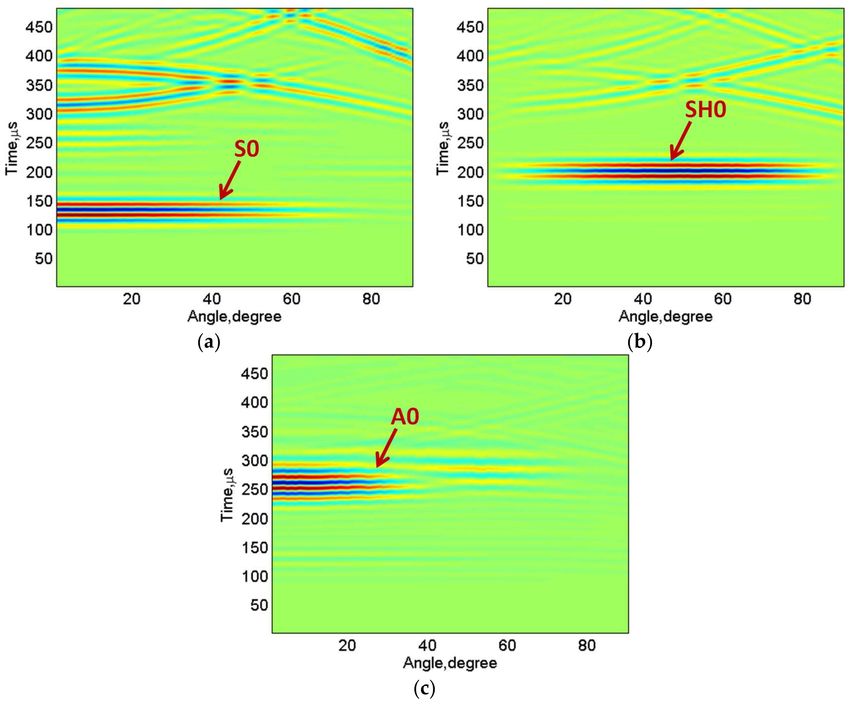
Sensors 2018, 18, 987                                                                                              2 of 17

transducer and object. Moreover, the contact transducers can be easily designed, configured or
adjusted depending on the type of defects or damages and the availability of access region of the
structure. Thus, the contact transducers are widely used in the various field of NDT such as the
detection of flaws with straight beam test, inspection of delamination or disbonds in composites
and many thickness gauging applications [10–13]. In this research work, the focus was kept on the
contact-type ultrasonic transducers for the generation of GWs.
      The contact-type ultrasonic transducers or the transducers glued to the surface of the structure
generating the GWs are required for the accurate inspection of the defects at larger propagation
distances from a fixed location on the structure. For a specific medium, a transducer operating as
a transmitter or a receiver has a unique directivity pattern. The transducer beam width for a particular
medium is the ratio of its diameter to the operating wavelength of UGW. Thus, a transducer with larger
size (diameter) produces a narrower beam in comparison to the smaller sized transducers. The major
amount of wave energy is contained by the main lobe of a directivity pattern while side lobes signify
the undesired radiations, reflections etc.
      Figure 1 shows a transducer glued on an object under inspection to demonstrate the effect of directivity
pattern on the probability of the defect estimation. The directivity pattern as a function of polar angle is also
illustrated to show the region of maximum radiation (main lobe) and the undesired radiations (side lobes).
It can be clearly observed from Figure 1 that defect-A and defect-C cannot be inspected from the presented
arrangement of the transmitting transducer as they are not in the region of coverage (directivity) of the
transducer. Hence, in order to analyze the parameters of defects A and C, the directivity pattern should be
altered. It can be achieved by selecting the one or more of the following options.

•     The location of the transducer can be changed;
•     The excitation frequency of a transducer can be changed;
•     The type of wave mode (e.g., the S0, A0 or SH0 in low-frequency (LF) ultrasonic) can be changed;
•     The utilization of the transducers array or different configuration of transducers can also be
      an alternative;

      Figure 1. Explaining the directivity pattern of a directional transducer glued on the object under inspection.

     Therefore, its directivity pattern is one of the most important characteristics of a transducer.
A prior information about the directivity pattern of a transducer before its usage can contribute to
choosing a suitable excitation frequency at which a transducer must be excited and appropriate wave
mode for the analysis of defects using ultrasonic non-destructive testing (NDT). It also leads to select
the optimum number of transducers or configuration of transducers to be used for the testing of
large and complex structures. This leads to reduce the overall cost of the SHM system. Moreover,
the transmitting wave modes (the S0, A0 or SH0 in the case of LF ultrasonic) of interest can also be
chosen as per requirements. Hence, the transmission/reception of unwanted wave modes can be
avoided in order to minimise the coherent noise.
     There are many theoretical, numerical and practical approaches developed for the analysis of directivity
patterns of ultrasonic transducers [14–18]. Haig et al. estimated the directivity patterns of the S0, A0 and
SH0 wave modes for macro-fiber composite (MFC) transducer glued on 10 mm thick steel plate using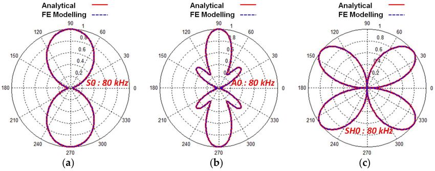
Sensors 2018, 18, 987                                                                                   3 of 17

finite element (FE) modelling, and further validated by the experimental analysis [19]. In the latest research
performed by Lowe et al. the behavior and directivity patterns of a flexible shear mode transducer were
analysed by FE modelling and laboratory experiments for the SHM applications using LF guided waves [20].
Conjusteau et al. demonstrated the applicability of directivity information in the quantitative tomography
and the construction of optoacoustic images [21]. Conjusteau et al. measured the spectral directivity
of ultrasonic transducers with a laser point source in order to construct the optoacoustic image [21].
The required directivity can also be achieved by forming the array of transducers. Wang et al. found that
the weaker directivity of micro-electromechanical systems (MEMS)-based capacitive ultrasonic transducer
can be significantly increased by forming a linear array of such transducers [22].
      The previously developed FE and experimental methods are limited to transducers of a specific
shape and configuration, the dispersive characteristics of the propagation medium and the excitation
frequency. Moreover, the numerical models and experimental analysis to predict the directivity
patterns of a transducer takes much longer time as compared to the analytical approach. Therefore,
a simplified, versatile and fast processing analytical model in order to predict the directivity pattern of
any contact-type ultrasonic transducer in any medium of know dispersive characteristics was required
to improve the ultrasonic NDT and SHM of the structures.
      The objective of the presented research work was to develop an efficient and fast processing 2D
analytical model for the estimation of directivity pattern of contact-type ultrasonic transducer by knowing
the behavior of a transducer and dispersive characteristics of the propagating medium. The transducer may
be of any shape and can be excited at any frequency. This work is the extension of a previously published
research article in the conference proceeding [23]. The article is organized as follows. Section 2 demonstrates
the procedure for the development of the 2D analytical model and its explanation by analyzing the P1-type
macro-fiber composite (MFC) transducer glued on an Al alloy plate. The finite element (FE) modelling
using ANSYS for the verification of results is explained in Section 3. The experimental approach with special
scanning and signal processing methods to estimate the directivity characteristics (only for the A0 Lamb
mode) is described in Section 4. The directivity patterns obtained by the developed analytical and numerical
modelling along with its comparison with the experimental results are demonstrated in Section 5. Finally,
the conclusions of the research are presented in Section 6.

2. Development of 2D Analytical Model
     A versatile and simplified 2D analytical model based on Huygens’s principle was developed.
The model can estimate and predict the directivity patterns of arbitrary contact-type GW transducers
in any propagation medium, at any excitation frequency, and at any distance assuming that the behavioral
characteristics of transducer and dispersive characteristics of the propagating medium are known. Based
on the Huygens’s principle proposed by C. Huygens, the points on the wavefront can be assumed as the
sources of wavelets which travel with the velocities of excited wave modes [24,25]. The basic methodology
and specific underlying assumptions associated with the analytical modelling are described as follows:

•     The ultrasonic contact type transducer of any shape and size can be assumed as uniformly
      distributed point sources on a 2D surface.
•     Create the equally spaced arbitrarily receiving points (elements) along the half-circle (0◦ to 180◦ )
      at the required distance (radius) from the center of the transducer (origin).
•     Calculate the distance vectors from all point sources to each arbitrary receiving element and
      integrate them.
•     Compute the theoretical phase velocity characteristics of the propagating modes in a medium by
      the “Disperse” [26] computational package.
•     Calculate the transfer function which is the multiplication of phase and attenuation components
      and depends on the excitation frequency, distance vector and the phase velocity of the propagating
      wave modes.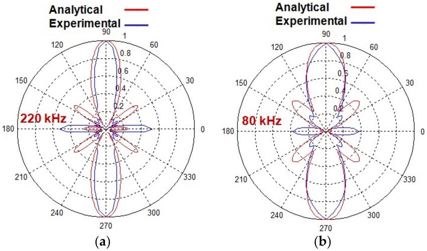
Sensors 2018, 18, 987                                                                                          4 of 17

•     The input signal is necessary to be multiplied by the correction factor (amplitude factor and
      direction factor). The amplitude factor depends on the type of propagating modes (e.g., the S0, A0,
      and SH0 in LF ultrasonic) and describes the signal distribution along the structure of transducer.
      The direction factor corresponds to the direction of propagating wave modes. The detailed
      description of the correction factor is discussed in Section 2.1.
•     Take an account the diffraction in distances and calculate the distance diffraction factor.
•     Calculate the output spectrum by multiplying the transfer function, corrected input signal
      spectrum (Fourier transform of the input signal after multiplying by correction factor) and
      the distance-dependent diffraction factor.
•     Calculate the output signal (B-scan or series of A-scans) in time-domain to estimate the directivity
      pattern of a transducer (by plotting the normalized peak-to-peak amplitudes of the propagating
      particular modes in the polar coordinates).

2.1. Description of 2D Analytical Modelling
     The description of the model is illustrated in Figure 2. It should be noted that a transducer with
a rectangular shape is analyzed in the analytical model. However, the basic principle entirely depends
on the calculation of distances between the point sources on the 2D surface of the transducer and
the arbitrary receiving points. Thus, the model will work for the transducer possessing any shape
and configuration. The two-dimensional (2D) coordinate system was used in modelling and origin
was assumed to be at the center of the transducer. The length (L) and width (w) of the rectangular
transducer section are in the direction along the y-axis and x-axis respectively.
     The transducer section was divided into n different line segments (n = 1, 2 ... N) with the step size
of dL along its length (L). In order to form the point sources along the 2D structure of a transducer,
each of the line segments was split into a series of m points (m = 1, 2 ... M) with the separation distance
of dw along the width. The coordinates of the transmitting point sources (xm , yn ) are described as [23]:

                             xm = (m − 1) · dw − w/2, yn = (n − 1) · dL − L/2                                     (1)

      It should be noted that high resolution in the results (directivity patterns) can be achieved by
keeping the dL and dw as shorter as possible. On another hand, simulation time of the model can be
reduced with higher values of the dL and dw. Therefore, an optimal value can be selected depending
on the spatial size of transducer considered for the modelling.
      The k arbitrary receiving elements (k = 1, 2 ..., K) were created along the half-circle of radius R from
the origin (center of the transducer) to construct the directivity pattern in the polar coordinates. If θk is the
angular position of receiving points along the half circle (0◦ to 180◦ ) with respect to the origin (θk = [(k−1) ·dθ],
dθ is the angular step), the coordinates of receiving elements can be expressed as [23]:

                                        xk = R · cos(θk ), yk = R · sin(θk )                                      (2)

                                 Figure 2. Description of 2D analytical modelling.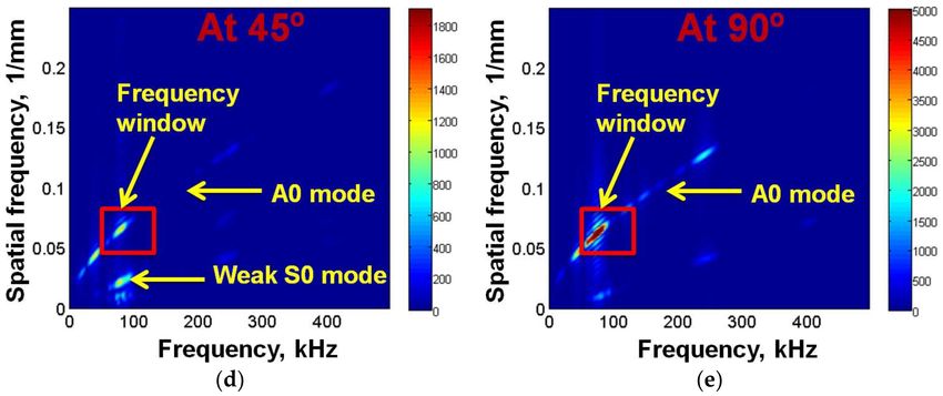
Sensors 2018, 18, 987                                                                                                     5 of 17

      In the next step, the distance between the point sources to each receiving point was calculated.
The distance vector (dk,n,m ) to the kth receiving element from the mth point source presented on the nth
line segment of the transducer and the respective angles (θ k,n,m ) were calculated as follows:
                                                       q
                                       dk,n,m =            ( x k − x m )2 + ( y k − y n )2                                   (3)

                                                                         yk − yn

                                                 θk,n,m = tan−1                                                              (4)
                                                                         xk − xm
      The transfer function H (f, dk,n,m , Vph ) was estimated as [27]:

                                                                                           2·π · f ·dk,n,m
                                                                                      −j
                                                                −α( f )·dk,n,m               Vph ( f ,h)
                               HT ( f , dk,n,m , Vph ) = e                       ·e                                          (5)

where α(f ) is the attenuation coefficient which is frequency (f ) dependent and can be assumed to be
zero for the isotropic lossless medium, VPh is the phase velocity which depends on the excitation
frequency (f ) and the thickness (h) of the propagation medium.
     Depending on the propagating GW wave modes, the correction factor (CF ) to be multiplied to the
input excitation signal uE (t) can be calculated as follows:

                                                   CF = A F · DF (θk,n,m )                                                   (6)

where AF is the amplitude factor which depends on the signal distribution along the structure of
a transducer, DF is the direction factor which is the function of θ k,n,m for a specific GW mode.
     The corrected input signal (uEC (t)) corresponding to the particular GW mode can be calculated as:

                                                   u EC (t) = u E (t) · CF                                                   (7)

      The output signal in the frequency domain at kth receiving element is then calculated as:

                                             N     M
                                                                                                                  1
                        UR,k ( f , θk ) =   ∑ ∑         UEC ( f ) · HT ( f , dk,n,m , Vp h ) · p
                                                                                                                 dk,n,m
                                                                                                                             (8)
                                            n =1 m =1

where UEC (f) is the spectrum of the corrected input signal uEC (t) which is calculated by obtaining
the Fourier transform (UEC (f) = FT [uEC (t)]), UR,k (f, θ k ) is the spectrum of the received signal at
                                                                                  √
kth receiving element, θ k is the angle in degree at kth receiving point and 1/ dk,n,m is the distance
diffraction factor [28].
     The inverse Fourier transform (FT−1 ) is then applied to construct the waveform of the received
signal at kth receiving element in the time domain:

                                            u R,k (t, θk ) = FT −1 [UR,k ( f , θk )]                                         (9)

     The peak-to-peak amplitudes (App (θ k )) and the normalized peak-to-peak amplitudes of the A-scan
signals (Anpp (θ k )) at the receiving points can be calculated as follows:

                                A pp (θk ) = max[u R,k (t, θk )] − min[u R,k (t, θk )]                                     (10)

                                                            A pp (θk )

                                             Anpp (θk ) =                                                                  (11)
                                                          max[ A pp (θk )]
    The normalized amplitude Anpp (θ k ) can be plotted in the polar coordinate system by varying the
angle θ k , from 0◦ to 180◦ in order to construct the directivity pattern for a specific GW mode.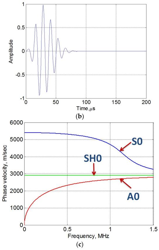
Sensors 2018, 18, 987                                                                            6 of 17

2.2. Demonstration of Analytical Model in the Case of P1-Type MFC Transducer
     In order to demonstrate the model for practical applications, the MFC transducer manufactured
by Smart Material Corporation [29] was analyzed to estimate the directivity patterns by the proposed
analytical model. The MFC consists of rectangular piezoceramic fiber rods, which are sandwiched
between layers of electrodes. These electrodes basically make an interdigitated pattern so that voltage
can be transferred to and from the rods. As MFC is a thin, low weight, flexible and easily molded
small sheet, it can be mounted/glued to the surface of the object or embedded into the multi-layered
composite structures of arbitrary configuration. Generally, MFCs operate in two modes: d33 mode
or elongation and d31 mode or contraction [29]. In this research work, P1-type MFC transducer
(M-2814-P1) with dimensions (28 × 14 mm) was selected which operates in d33 (elongation) mode
and can actuate and sense ultrasonic waves along the length of the MFC. One of the best features of
MFC transducer is that MFC is an efficient transmitter and receiver of the asymmetric (A0) and the
symmetric (S0) modes of guided Lamb waves at LF ultrasonic [30,31]. Apart from the fundamental
Lamb wave modes (the A0 and S0), the fundamental shear horizontal mode (SH0) is another kind of
guided wave which is completely non-dispersive [19]. The S0 (in the direction of wave propagation)
and SH0 (in the perpendicular direction of wave propagation) modes are mainly distributed in-plane
and the A0 mode is out-of-plane. As P1-type MFC operates in elongation mode, the S0 mode is the
most dominant.
     The task was to calculate the directivity of P1-type MFC transducer glued on 2 mm thick aluminum
(Al) alloy plate at the distance of 300 mm from the center of MFC transducer in the generation of GW
modes (the S0, A0, and SH0). The plate of Al alloy was assumed to be infinite dimensions, therefore
the length and width of it are not considered. The transducer was excited using 80 kHz, 5-period
burst signal with a Gaussian envelope and the sampling frequency of 1.6 MHz was used to record
the received samples. A photo image of the MFC transducer, excitation signal and the phase velocity
dispersion curves of the GW modes in 2 mm Al plate are shown in Figure 3. The phase velocities
of the S0, SH0 and A0 modes at 80 kHz excitation frequency were estimated as 5409 m/s, 2903 m/s,
and 1183 m/s respectively.

                                            Figure 3. Cont.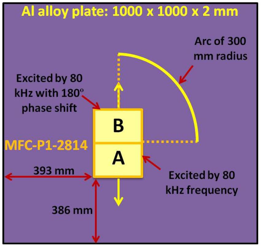
Sensors 2018, 18, 987                                                                                             7 of 17

      Figure 3. MFC transducer and guided waves: photo of P1-type MFC transducer (a), excitation signal of
      80 kHz, 5-period burst (b) and phase velocity dispersion curves of GW modes in 2 mm thick Al alloy plate (c).

     The MFC transducer was divided into 29 equal segments along its length (28 mm) with
a separation distance of 1 mm. Each segment was analyzed as the 15 point sources along the
width (14 mm) of MFC which lead the total number of point sources along the structure equal
to 435. On another hand, total 181 arbitrary receiving elements placed at a distance of 300 mm
from the center of MFC were located along the half-circle at the angular positions varying from
0◦ to 180◦ . The attenuation coefficient α(f ) was assumed to be zero for the Al (isotropic and lossless
medium) plate. The correction factor (CF ) to be included for the specific mode is described in Figure 4.
Figure 4a illustrates that the particle displacements in both halves of the P1-type MFC are in opposite
direction along its length (in y-axis) due to its operation in elongation (d33) mode. Hence the
approximated value of the amplitude factor (AF ) was assumed to be equal to 1 and −1 at the edges of
MFC (all point sources of first and last line segments) along its length (y-axis) which was decreased
linearly towards the axis (center of MFC) where its value was set to zero.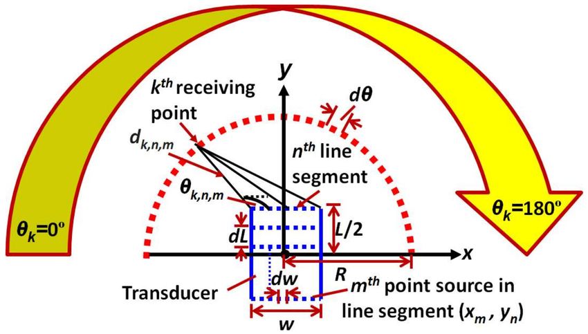
Sensors 2018, 18, 987                                                                                      8 of 17

      Figure 4. Calculation of correction factor (CF ) for P1-MFC transducer: The particle displacements in
      excited P1-type MFC transducer (a), The correction factor CF (multiplication of the amplitude factor
      (AF ) and direction factor for a specific GW mode (A0 or S0)) (b).

     For the estimation of the direction factor (DF ), the theory of GW modes and the behavior of
transducer were utilized. If θ k,n,m is the angle between the point source and a receiving element,
the direction factor (DF ) for the S0 and SH0 will be calculated by sin (θ k,n,m ) and cos (θ k,n,m ) respectively
and illustrated in Figure 4b. The direction factor DF for the out-of-plane A0 mode will be unity. Therefore,
the correction factor (CF ) for each mode was calculated from Equation (6) as [32,33]:

               CF (S0) = A F (y) · sin(θk,n,m ),CF (SH0) = A F (y) · cos(θk,n,m ), CF ( A0) = A F (y)         (12)

3. Numerical Simulation Using FE
     The numerical simulation was performed by developing the finite element (FE) model using the
“ANSYS” commercial software for the verification of analytical results. The 3D model of Al-alloy
plate (1000 × 1000 × 2 mm) with the mechanical properties incorporated in Table 1 was developed
using SOLID 64 elements which are widely used for three-dimensional modelling of solid structures.
Each element contained 8 nodes with a degree of freedom (DOF) equals to three: translation in x, y and
z directions. Each element size was 1 mm. It should be noted that MFC was not modeled explicitly
and only the behavior of the MFC was analyzed in order to develop the transducer section on Al alloy
plate [34]. The appropriate force (excitation signal) of a five-period burst and frequency of 80 kHz with
the Gaussian envelope (Figure 3b) was applied for investigating the wave propagation effects at the
distance of 300 mm from the center of MFC transducer.

                                 Table 1. Mechanical properties of Al-alloy plate.

                                Symbol          Quantity         Numerical Value
                                    E       Young’s modulus           71 GPa
                                    ρ           Density             2780 kg m−3
                                    υ        Poisson’s ratio            0.33

    For the calculation of directivity pattern, it was required that excitation zone and its behavior
should be similar to the MFC-P1-2814. As the MFC-P1-2814 works in elongation or d33 mode, the upper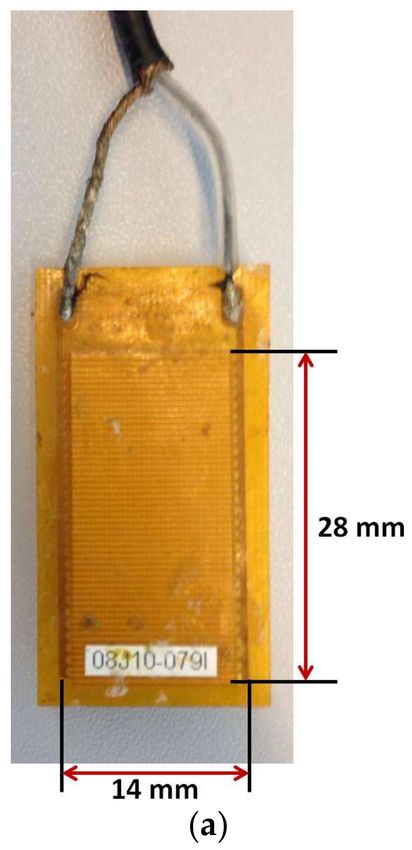
Sensors 2018, 18, 987                                                                              9 of 17

and lower half of MFC transducer (28 × 14 mm) was excited by 80 kHz signals but in opposite phase.
The sampling frequency was kept at 1.6 MHz. Due to symmetry associated with MFC structure and
for shortening the simulation time, only a quarter-circle of 300 mm radius was selected to locate the
receiving elements as illustrated in Figure 5. The transmitting zone (MFC) was positioned at 393 mm
distance from the left side and at 386 mm distance from the bottom side of Al plate. The post-processing
and the node selection to develop the quarter arc of 300 mm radius were performed in MATLAB.
     The solution was obtained using numerical integration and in this way, the particle velocity
distribution in the whole simulated structure at different time instants was obtained. To construct
the directivity pattern of S0 mode and SH0 mode, the resultant particle velocity signals (in-plane)
in direction of propagation and in the perpendicular direction to the propagation had to be
determined. The out-of-plane signal to construct the directivity pattern of the A0 mode was the
same as a y-component signal of the ANSYS model. The calculation of resultant signals to construct
the directivity pattern is presented in Figure 6.
     Let assume, that Sz , Sx, and Sy are the three components of received particle velocity signals in
the z-direction (along with the length of MFC), x-direction (along with the width of MFC) and in
the y-direction (out-of-plane) respectively at the receiving points along the arc of 30 cm in ANSYS 3D
modelling. These signal components are shown in Figure 6a. It must be noted that resultant out-of-plane
signal (RA0 ) to construct the directivity pattern of A0 mode was equal to the Sy. The in-plane resultant
signals in the direction of propagation (RS0 ) and perpendicular to the direction of propagation (RSH0 )
were calculated by analyzing the projection of Sz and Sx on RS0 and RSH0 respectively. The graphical
representation to calculate these signals are shown in Figure 6b and can be described as follows [25,26]:

                                       RS0 = Sz · sin θ + Sx · cos θ                                   (13)

                                      RSH0 = Sz · cos θ − Sx · sin θ                                   (14)

                                                R A0 = Sy                                              (15)

where θ is the angle in degree from positive x-axis to the direction of wave propagation.

      Figure 5. Description of numerical modelling of P1-type MFC transducer glued on Al alloy plate
      using FE.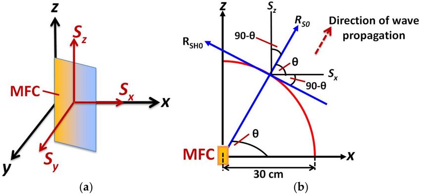
Sensors 2018, 18, 987                                                                                             10 of 17

      Figure 6. Calculation of resultant signals in FE numerical modelling: Showing signal components of
      particle velocity (Sx, , Sy and Sz ) along the axis (a) and resultant/received signals in the direction of
      propagation (RS0 ) and perpendicular to the direction of propagation (RSH0 ) (b).

     The B-scans images of the S0 (the signal RS0 ), SH0 (the signal RSH0 ) and A0 (the signal RA0 ) waves
were acquired in the computational package MATLAB and shown in Figure 7a–c. It can be clearly
observed that the S0 mode was the fastest with an approximate time of arrival of 100 µs and the
A0 was the slowest with an approximate time of arrival 225 µs. By applying the appropriate time
windows on the respective B-scans, each mode (the S0, A0 or SH0) can be extracted to construct the
directivity patterns.

      Figure 7. The B-scan images of particle velocity components in the direction of propagation (the S0) (a),
      perpendicular to the direction of propagation (the SH0) (b), and in the direction of propagation (the A0) (c).
Sensors 2018, 18, 987 11 of 17
4. Experimental Investigation
In order to validate the results obtained by the analytical and FE modelling, the experimental
investigation was performed to estimate the directivity of P1-type MFC transducer glued at the center
of Al alloy plate. The mechanical properties and the geometry of the Al alloy plate were similar as
described in the part of FE modelling (Section 3). The signal of 5-period burst, amplitude of 20 V and
frequency of 80 kHz was used to excite the MFC transducer. During the experiments, the point-type
wideband ultrasonic transducer with a conical protection layer (diameter < 0.3 mm) and bandwidth
up to 350 kHz at −6 dB level was used as a contact type receiver to receive the GW modes at 100 MHz
sampling frequency with minimum distortions [11]. The mechanical scanning unit was used for the
positioning of the receiving transducer in the polar coordinate system.
As the point-type receiver operates in thickness mode, the A0 mode in comparison to other
modes was captured more effectively. Therefore, during experiments, the directivity of only A0
mode was estimated for the comparative analysis with the modelling results. The experimental
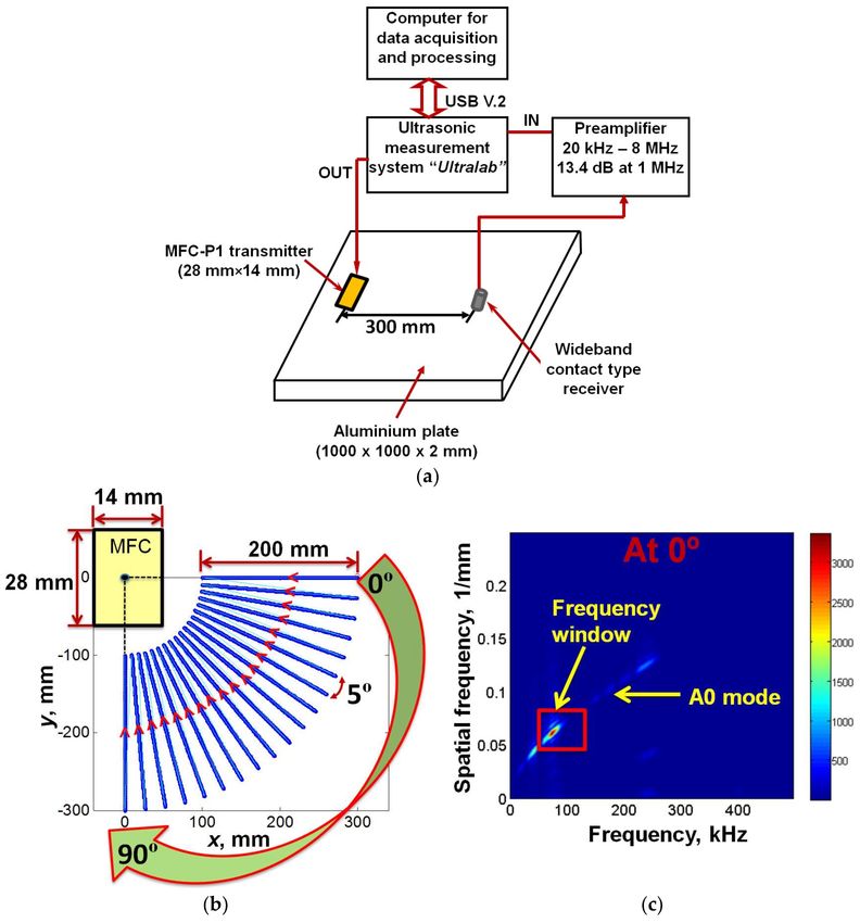
set-up is shown in Figure 8a. The experiment was performed using the Ultralab low-frequency
(LF) ultrasonic measurement system, which has been developed at Ultrasound Institute of Kaunas
University of Technology.
Figure 8. Cont.Sensors 2018, 18, 987 12 of 17
Figure 8. Experimental analysis and post-processing: Experimental set-up showing the glued MFC on
Al alloy plate and the initial position of a point-type contact transducer (dimensions are not in scale)
connected with LF ultrasonic system (a), showing the scanning process to acquire 19 B-scans at each
5◦ in the angular direction from 0◦ to 90◦ (b), showing the application of frequency window on the
dispersion curves of the first (at 0◦ ), tenth (at 45◦ ) and nineteenth (at 90◦ ) B-scans for selecting the
appropriate signals at excitation frequency of 80 kHz (c–e).
The pitch-catch technique (MFC transmitter was fixed and receiving transducer was scanned) was
performed for the experiment as only one side of the object had to be accessed during the experimental
investigation. The receiving transducer was initially positioned at 300 mm from the MFC along its
width. The received signals were acquired along the quarter circle (0 to 90◦ ) to construct the directivity
pattern of the A0 mode. In order to capture the GW modes with minimum interference of neighboring
modes and minimum distortion, a special scanning procedure and signal processing was used as
illustrated in Figure 8b–e. The entire process can be described as follows:
• The quarter circle having the radius of 300 mm and the angular direction from 0 to 90◦ was
divided into the 19 points located at each 5◦ as shown in Figure 8b. The linear scanning was
performed by moving the contact-type transducer up to the 200 mm with a scanning step of
0.5 mm from each point towards the MFC transducer.
• In this way, 19 B-scan images were recorded in total within the angular direction from 0◦ to 90◦ .
The sampling frequency of 100 MHz was used.
• The two-dimensional Fourier transform (2D-FFT) was applied to each B-scan for the transformation of
measurements in distance-time into the spatial frequency-frequency [32,35]. Figure 8c–e shows the
dispersion curve generated after applying the 2D-FFT on first B-scan (at 0◦ ), tenth B-scan (at 45◦ ) and
nineteenth B-scan (at 90◦ ).
• Although the propagation medium (Al alloy) is isotropic, the MFC is not a point-type transducer and
generates not only the fundamental guided Lamb modes (the S0 and A0) but the non-dispersive GW
mode (the SH0) is also generated. Therefore, the dispersive characteristics obtained for all 19 B-scans
were not similar. In order to select the signals of interest, a rectangular window within the frequency
range of 60–110 kHz and spatial frequency range of 0.04–0.075 1/mm was applied on each of the
transformed B-scan signal (2D-FFT). The window was selected in such a manner that possible values
of signal energies in each case were contained. The application of frequency window on the dispersion
curves of the first (at 0◦ ), tenth (at 45◦ ) and nineteenth (at 90◦ ) B-scans are shown in Figure 8b–e.
• Finally, the maximum energy of all 19 signals in the selected window was estimated in order to
construct the directivity pattern in the polar coordinates (from 0◦ to 90◦ ).
The experiment and the signal processing was repeated for the excitation signal of 220 kHz, 5-period.Sensors 2018, 18, 987 13 of 17
5. Results
The directivity characteristics of GW modes possessing in-plane components (the S0 and SH0)
and out-of-plane components (the A0) were estimated at 80 kHz, 5-period excitation signal in the case
of P1-type MFC transducer glued on 2 mm Al alloy plate. The normalized directivity characteristics
obtained from the analytical modelling (Section 2.2) and FE (Section 3) analysis were exactly matched
as shown in Figure 9. It should be noted that directivity patterns were constructed and plotted in
the polar coordinates from 0◦ to 360◦ . The symmetry of the MFC structure facilitated to utilize the
mirror image of pattern across the axes. It means that directivity characteristics calculated in the
polar coordinates from 0 to 90◦ are similar to those calculated from 270◦ to 360◦ . In a similar way,
the directivity characteristics obtained in the polar coordinates from 0◦ to 180◦ would be similar to
those calculated in the range from 180◦ to 360◦ .
Figure 9. Normalized directivity characteristics of the S0 (a), A0 (b) and SH0 (c) guided wave modes
at 80 kHz, 5-period excitation signal for the P1-type MFC transducer glued on 2 mm Al alloy plate
obtained by analytical and FE modelling.
The P1-type MFC operates in the elongation or d33 mode. Hence, the GW mode in the direction
of propagation (the S0) is most dominant and directional in comparison to the A0 and the SH0 mode
(Figure 9a–c). As shown in Figure 9a, the most of the wave energy associated with the S0 and A0
modes was observed towards 0◦ and 90◦ (longitudinal or in the direction of propagation). However,
the A0 mode contained the side lobes with significant beam-width at 40◦ , 140◦ , 220◦ and 320◦ and
the smaller side lobes at 0 and 180◦ apart from the major lobes (Figure 9b). The beam-width of major
lobes in the case of A0 was also narrower as compared to the S0 mode. The number of wavelengths (λ)
or signal distributions along the dimension of the transducer has an important role in the shape of
directivity patterns. For the 80 kHz frequency, the wavelength for the S0 mode (λ = 67 mm) is almost
2.5 times of the length (28 mm) of MFC transducer. On another hand, it is equal to almost half of the
length of MFC (λ = 14.83 mm) in the case of A0 mode. Although SH0 travels along the perpendicular
direction of wave propagation (along the width of MFC) but upper and lower halves of MFC vibrating
in opposite directions suppress the wave intensity along the 0◦ and 180◦ and therefore the SH0 waves
possess the wave intensities at 40◦ , 140◦ , 220◦ and 320◦ in the resulting pattern (Figure 9c). Thus,
the specific directivity characteristics of the SH0 mode are necessary to be taken into account during
application of P1-type MFC transducers in NDT tasks.
The experimental result of the directivity pattern (only for the A0) was obtained at 80 kHz and
5-period excitation signal in order to perform the comparison with the results obtained by analytical
modelling. The comparative result is shown in Figure 10a. The analytical results exhibit the sufficient
resemblance with the results obtained from the experimental investigation. The same number of
lobes (2 major lobes at 90◦ and 180◦ and 6 side lobes at 0◦ , 40◦ , 140◦ , 220◦ and 320◦ ) is visible in bothSensors 2018, 18, 987 14 of 17
patterns. The size and shape of the major lobes in both analytical and experimental results were almost
similar but the significant variation in the size of side lobes was observed. At 0◦ and 180◦ , side lobes
possessing more wave energy was observed in the experimental directivity pattern as compared to the
analytical result. On another hand, the analytical results exhibited the more wave energy of side lobes
at 40◦ , 140◦ , 220◦ and 320◦ .
The experimental analysis described in Section 4 was repeated again by exciting the MFC
transducer at 220 kHz and 5-period excitation signal. The comparison of the experimentally and
analytically obtained directivity patterns for the A0 mode at 220 kHz is shown in Figure 10b. The shape
of major lobes and number of lobes of both directivity patterns are sufficiently matched but as observed
in Figure 10a, the size of side lobes does not show the significant similarities. However, the analytical
result again shows the good compromise with the experimental result. Although beam width of
the major lobe at 220 kHz (Figure 10b) is narrower as compared to that of 80 kHz (Figure 10a),
the number of side lobes is increased. The number of side lobes in the case of 220 kHz was observed
as 10. The difference between the analytical and experimental results is due to the fact that the
signal distributions (Amplitude correction factor (AF )) along the structure of MFC transducer were
approximately considered depending on the behaviour of the transducer. The consideration of wave
patterns (signal wavelengths) along the structure of transducer could improve the results of analytical
modelling in future research.
Figure 10. Comparative analysis of normalized directivity patterns of the A0 wave mode obtained
by analytical modelling and experimental investigation at 80 kHz, 5-period excitation signal (a) and
220 kHz, 5-period excitation signal (b).
6. Conclusions
The fast processing 2D analytical model has been developed in order to predict the directivity
patterns of contact type ultrasonic transducers by knowing the behavior of the transducer and the
dispersive characteristics of the propagating medium. The model is valid to estimate the directivity
pattern at any distance excitation frequency. The proposed model will not only facilitate to select
the position and the number of transducers but also leads to selecting the specific transducer and
wave modes for the inspection of a particular type of defects using ultrasonic NDT. The novelty of the
presented research work can be summarized as follows:
• Development of a 2D analytical model of contact type transducers based on Huygens’s principle
capable to draw the directivity patterns within a far shorter processing time as compared to the
finite element modelling and experimental investigation.Sensors 2018, 18, 987 15 of 17
• Explanation of model for p1-type macro fiber composite (P1-type MFC) transducer manufactured
by Smart Material excited by 80 kHz, 5-period excitation signal. The propagation medium was
2 mm aluminum alloy plate. Verification of the results was performed using FE modelling.
• Special experimental scanning and signal processing approach was also proposed in order to
estimate the directivity patterns of P1-type MFC transducer glued on 2 mm Al alloy plate and
exciting the fundamental modes with the lower interference of additional reverberations.
The directivity patterns of the S0, A0 and SH0 modes generated by P1-type MFC transducer at
80 kHz frequency were perfectly matched with the results obtained using FE modelling.
The directivity patterns of the A0 mode estimated by experimental investigation at 80 kHz and
220 kHz excitation frequencies were also similar to the analytical results except for the small differences
in the beam-width of the main lobe and length of the side lobes. The reasons for differences are related
to the signal distribution along the MFC structure and the amplitude correction factor (AF ) assumed
in the development of analytical modelling. The approximated magnitudes of amplitude correction
factor were assumed in the analytical modelling in accordance with the expected behavior of the
transducer. In the future research, the signal distributions along the structure of MFC transducer can
be improved by analyzing the number of signal wavelengths of propagating fundamental modes
in more details and therefore the accuracy for setting the values of amplitude correction factor can
be increased. Moreover, it should be noted that the total simulation time of the proposed analytical
model was significantly shorter in comparison to the time spent on experimental investigation and
FE modelling.
Acknowledgments: This work was performed at Ultrasound Research Institute of the Kaunas University of
Technology, Lithuania.
Author Contributions: Kumar Anubhav Tiwari developed the analytical model and implemented the algorithm
in MATLAB, performed the experimental investigation, analysed the numerical simulation results in MATLAB
and wrote the manuscript. Renaldas Raisutis contributed to the experimental analysis, edited the article and
supervised the entire research. Liudas Mazeika helped and guided to develop the analytical model, helped for
the post-processing of results of numerical simulation in MATLAB. Vykintas Samaitis performed the numerical
simulations in ANSYS.
Conflicts of Interest: The authors declare no conflict of interest.
References
1. Mitra, M.; Gopalakrishnan, S. Guided wave based structural health monitoring: A review. Smart Mater. Struct.
2016, 25, 053001. [CrossRef]
2. Raghavan, A.; Cesnik, C.E.S.; Raghavan, A.; Cesnik, C.E.S. Review of Guided-Wave Structural Health
Monitoring. Shock Vib. Dig. 2007, 39, 91–114. [CrossRef]
3. Draudvilienė, L.; Raišutis, R.; Žukauskas, E.; Jankauskas, A. Validation of Dispersion Curve Construction
Techniques for the A0 and S0 Modes of Lamb Waves. Int. J. Struct. Stab. Dyn. 2014, 14, 1450024. [CrossRef]
4. Toyama, N.; Takatsubo, J. Lamb wave method for quick inspection of impact-induced delamination in
composite laminates. Compos. Sci. Technol. 2004, 64, 1293–1300. [CrossRef]
5. Edalati, K.; Kermani, A.; Seiedi, M.; Movafeghi, A. Defect detection in thin plates by ultrasonic lamb wave
techniques. Int. J. Mater. Prod. Technol. 2006, 27, 156. [CrossRef]
6. Loveday, P.W.; Long, C.S. Long range guided wave defect monitoring in rail track. AIP Conf. Proc. 2014,
1581, 179–185. [CrossRef]
7. Zhang, K.; Han, Z.D.; Yuan, K.Y. Long Range Inspection of Rail-Break Using Ultrasonic Guided Wave Excited
by Pulse String. Adv. Mater. Res. 2013, 744, 505–510. [CrossRef]
8. Tiwari, K.; Raisutis, R. Comparative analysis of non-contact ultrasonic methods for defect estimation of
composites in remote areas. CBU Int. Conf. Proc. 2016, 4, 846–851. [CrossRef]
9. Nakamura, K. Ultrasonic Transducers: Materials and Design for Sensors, Actuators and Medical Applications;
Woodhead Publishing: Cambridge, UK, 2012; Volume 1, pp. 3–183. ISBN 9781845699895.
10. Liu, T.; Kitipornchai, S.; Veidt, M. Analysis of acousto-ultrasonic characteristics for contact-type transducers
coupled to composite laminated plates. Int. J. Mech. Sci. 2003, 43, 1441–1456. [CrossRef]Sensors 2018, 18, 987 16 of 17
11. Vladišauskas, A.; Šliteris, R.; Raišutis, R.; Seniūnas, G.; Žukauskas, E. Contact ultrasonic transducers for
mechanical scanning systems. Ultragarsas (Ultrasound) 2010, 65, 30–35.
12. Lee, J.R.; Park, C.Y.; Kong, C.W. Simultaneous active strain and ultrasonic measurement using fiber acoustic
wave piezoelectric transducers. Smart Struct. Syst. 2013, 11, 185–197. [CrossRef]
13. Tiwari, K.A.; Raisutis, R.; Samaitis, V. Hybrid Signal Processing Technique to Improve the Defect Estimation
in Ultrasonic Non-Destructive Testing of Composite Structures. Sensors 2017, 17, 2858. [CrossRef] [PubMed]
14. Qi, W.; Cao, W. Finite element study on 1-D array transducer design. IEEE Trans. Ultrason. Ferroelectr. Freq. Control
2000, 47, 949–955. [CrossRef] [PubMed]
15. Leeman, S.; Healey, A.J.; Costa, E.T.; Nicacio, H.; Dantas, R.G.; Maia, J.M. Measurement of transducer
directivity function. In Medical Imaging 2001: Ultrasonic Imaging and Signal Processing; International Society
for Optics and Photonics: Bellingham, WA, USA, 2001; Volume 4325, pp. 47–54.
16. Voelz, U. Four-dimensional directivity pattern for fast calculation of the sound field of a phased array
transducer. In Proceedings of the 2012 IEEE International Ultrasonics Symposium, Dresden, Germany,
7–10 October 2012; pp. 1035–1038.
17. Li, D.; Chen, H. Directivity calculation for acoustic transducer arrays with considering mutual radiation
impedance. In International Conference on Graphic and Image Processing (ICGIP 2012); International Society for
Optics and Photonics: Bellingham, WA, USA, 2013; Volume 8768, p. 876864.
18. Umchid, S. Directivity Pattern Measurement of Ultrasound Transducers. Int. J. Appl. Biomed. Eng. 2009, 2,
39–43.
19. Haig, A.; Sanderson, R.; Mudge, P.; Balachandran, W. Macro-fibre composite actuators for the transduction
of Lamb and horizontal shear ultrasonic guided waves. Insight-Non-Destr. Test. Cond. Monit. 2013, 55, 72–77.
[CrossRef]
20. Lowe, P.S.; Scholehwar, T.; Yau, J.; Kanfoud, J.; Gan, T.-H.; Selcuk, C. Flexible Shear Mode Transducer for
Structural Health Monitoring using Ultrasonic Guided Waves. IEEE Trans. Ind. Inform. 2017, PP. [CrossRef]
21. Conjusteau, A.; Ermilov, S.; Su, R.; Brecht, H.; Fronheiser, M.; Oraevsky, A. Measurement of the spectral
directivity of optoacoustic and ultrasonic transducers with a laser ultrasonic source. Rev. Sci. Instrum. 2009,
80, 093708. [CrossRef] [PubMed]
22. Wang, H.; Wang, X.; He, C.; Xue, C. Design and Performance Analysis of Capacitive Micromachined
Ultrasonic Transducer Linear Array. Micromachines 2014, 5, 420–431. [CrossRef]
23. Tiwari, K.A.; Raisutis, R.; Mazeika, L.; Samaitis, V. Development of a 2D analytical model for the prediction
of directivity pattern of transducers in the generation of guided wave modes. Procedia Struct. Integr. 2017, 5,
973–980. [CrossRef]
24. Jenkins, F.A.; Watson, W.W. Huygens’ principle. Access Sci. 2014. [CrossRef]
25. Coleman, C. Huygen’s principle applied to radio wave propagation. Radio Sci. 2002, 37. [CrossRef]
26. Pavlakovic, B.N.; Lowe, M.; Alleyne, D.; Cawley, P. Disperse: A general purpose program for creating
dispersion curves. In Annual Review of Progress in Quantitative NDE; Thompson, D.O., Chimenti, D.E., Eds.;
Plenum Press: New York, NY, USA, 1997; pp. 185–192. [CrossRef]
27. He, P. Simulation of ultrasound pulse propagation in lossy media obeying a frequency power law.
IEEE Trans. Ultrason. Ferroelectr. Freq. Control 1998, 45, 114–125. [CrossRef] [PubMed]
28. Morin, D. Interferance and Diffraction. In Waves; Harvard University Press: Cambridge, MA, USA, 2010;
Chapter 9; pp. 1–38. Available online: www.people.fas.harvard.edu/~djmorin/waves/interference.pdf
(accessed on 27 March 2016).
29. Macro Fiber Composite (MFC). Available online: http://www.smart-material.com/MFC-product-main.html
(accessed on 20 March 2017).
30. Wilkie, W.K.; Bryant, R.G.; High, J.W.; Fox, R.L.; Hellbaum, R.F.; Jalink, A.; Little, B.D.; Mirick, P.H. Low-cost
piezocomposite actuator for structural control applications. In Smart Structures and Materials 2000: Industrial
and Commercial Applications of Smart Structures Technologies; International Society for Optics and Photonics:
Bellingham, WA, USA, 2000; Volume 3991, pp. 323–335. [CrossRef]
31. Ren, G.; Jhang, K. Application of Macrofiber Composite for Smart Transducer of Lamb Wave Inspection.
Adv. Mater. Sci. Eng. 2013, 2013, 281575. [CrossRef]
32. Su, Z.; Ye, L.; Lu, Y. Guided Lamb waves for identification of damage in composite structures: A review.
J. Sound Vib. 2006, 295, 753–780. [CrossRef]Sensors 2018, 18, 987 17 of 17
33. Rose, J. Ultrasonic Waves in Solid Media; Cambridge University Press: Cambridge, UK, 2014; pp. 76–287.
ISBN 9781107273610.
34. Samaitis, V.; Mažeika, L. Influence of the Spatial Dimensions of Ultrasonic Transducers on the Frequency
Spectrum of Guided Waves. Sensors 2017, 17, 1825. [CrossRef] [PubMed]
35. Alleyne, D.; Cawley, P. A two-dimensional Fourier transform method for the measurement of propagating
multimode signals. J. Acoust. Soc. Am. 1991, 89, 1159–1168. [CrossRef]
© 2018 by the authors. Licensee MDPI, Basel, Switzerland. This article is an open access
article distributed under the terms and conditions of the Creative Commons Attribution
(CC BY) license (http://creativecommons.org/licenses/by/4.0/).You can also read