Ionospheric detection of gravity waves induced by tsunamis - CORE
←
→
Page content transcription
If your browser does not render page correctly, please read the page content below
Geophys. J. Int. (2005) 160, 840–848                                                                           doi: 10.1111/j.1365-246X.2005.02552.x

                 Ionospheric detection of gravity waves induced by tsunamis

                 Juliette Artru,1 Vesna Ducic,2 Hiroo Kanamori,1 Philippe Lognonné2
                 and Makoto Murakami3
                 1 SeismologicalLaboratory MC 252-21, California Institute of Technology, Pasadena, CA 91125, USA. E-mail: juliette@gps.caltech.edu
                 2 Institut
                          de Physique du Globe de Paris, Département de Géophysique Spatiale et Planétaire, UMR7096, 4 avenue de Neptune,
                 94107 Saint-Maur-des-Fossés, France
                 3 Crustal Deformation Laboratory, Geographical Survey Institute, Tsukuba, Japan

                 Accepted 2004 December 8. Received 2004 December 3; in original form 2004 July 23

                                                                                                                                                                        Downloaded from http://gji.oxfordjournals.org/ at California Institute of Technology on November 11, 2014
                                                        SUMMARY
                                                        Tsunami waves propagating across long distances in the open-ocean can induce atmospheric
                                                        gravity waves by dynamic coupling at the surface. In the period range 10 to 20 minutes, both
                                                        have very similar horizontal velocities, while the gravity wave propagates obliquely upward
                                                        with a vertical velocity of the order of 50 m s−1 , and reaches the ionosphere after a few hours. We
                                                        use ionospheric sounding technique from Global Positioning System to image a perturbation
                                                        possibly associated with a tsunami-gravity wave. The tsunami was produced after the M w =
                                                        8.2 earthquake in Peru on 2001 June 23, and it reached the coast of Japan some 22 hours later.
                                                        We used data from the GEONET network in Japan to image small-scale perturbations of the
                                                        Total Electron Content above Japan and up to 400 km off shore. We observed a short-scale
                                                        ionospheric perturbation that presents the expected characteristics of a coupled tsunami-gravity
                                                        wave. This first detection of the gravity wave induced by a tsunami opens new opportunities
                                                        for the application of ionospheric imaging to offshore detection of tsunamis.
GJI Seismology

                                                        Key words: atmospheres, Global Positioning System (GPS), ionosphere, tsunamis.

                                                                                               of 104 compared to the ground velocity, and is therefore detectable
                 1 I N T RO D U C T I O N
                                                                                               on ground-based or ground-satellite measurements (Blanc 1985).
                 Tsunamis are long surface gravity waves that propagate for great                 Tsunami waves are expected to induce a similar type of coupling
                 distances in the ocean. They are usually triggered by submarine               with the atmosphere: despite their small amplitude compared to
                 earthquakes, landslides or eruptions. While tide gauges can mea-              ocean swell, they can generate atmospheric gravity waves because
                 sure tsunami waves along the coast, detection and monitoring in               of their long wavelengths. The possibility of detection of tsunamis
                 the open ocean is very challenging due to the long wavelengths                by monitoring the ionospheric signature of the induced gravity wave
                 (typically 200 km) and small amplitudes (a few cm or less of sea              was proposed by Peltier & Hines (1976). They discussed the theo-
                 surface vertical displacement) compared to wind-generated waves.              retical issue of the coupling, and found that the several difficulties
                 Reported offshore detections involve ocean-bottom sensors (Hino               one would expect a priori should not have any major consequences
                 et al. 2001; Tanioka 1999) (pressure gauges or seismometers), sea             on the feasibility. We will recall their main conclusions in Sec-
                 level measurement from Global Positioning System receivers on                 tion 2.1. To our knowledge, however, no further attempt has been
                 buoys (Gonzalez et al. 1998; Kato et al. 2000) or satellite altimetry         performed. Part of the problem is certainly the lack of ionospheric
                 (Okal et al. 1999).                                                           measurements above the oceans, and also the difficulty to distinguish
                    Since the 1960s, numerous observations of acoustic-gravity                 tsunami-related gravity waves from any other source of traveling
                 waves in the ionosphere induced by solid Earth events, such as                ionospheric disturbances.
                 earthquakes, mine blasts or explosions, have been published (Bolt                More recently, the development of high-density Global Position-
                 1964; Harkrider 1964; Calais et al. 1998). They highlighted the gen-          ing System (GPS) networks have made a breakthrough in iono-
                 eration of such atmospheric waves at the Earth surface by vertical            spheric monitoring, allowing us to image propagation of Traveling
                 displacements with very small amplitude but large wave length, such           Ionospheric Disturbances (TIDs) over large areas. Calais & Minster
                 as seismic surface waves (Artru 2001; Artru et al. 2001). The main            (1998) detected ionospheric perturbations after the 1994 Northridge
                 reason for having such coupled solid-Earth atmosphere signals is              earthquake. The detection and imaging of Rayleigh waves after
                 that the exponential decrease of density with height causes an ex-            the 2002 Denali earthquake using California GPS networks (Ducic
                 ponential amplification of the atmospheric wave by conservation of            et al. 2003) showed that despite the fact that GPS measures the inte-
                 the kinetic energy. In the F region of the ionosphere (150–600 km of          grated electron density between the satellite and the receiver, small
                 altitude), the velocity perturbation is typically amplified by a factor       scale waves could be resolved and identified using adapted data

                 840
                                                                                                                                                         C   2005 RAS
Atmospheric gravity waves induced by tsunamis                 841

                                                                                                                                                         Downloaded from http://gji.oxfordjournals.org/ at California Institute of Technology on November 11, 2014
Figure 1. Schematic view of our study. The geometry of GPS measurements allows to detect ionospheric perturbations above the open ocean, and therefore
possible gravity waves induced by tsunamis.

processing. Moreover, the geometry of GPS ionospheric measure-
                                                                              2 T S U N A M I – I N T E R N A L G R AV I T Y
ments is particularly interesting for the detection of offshore signal:
                                                                              WAV E S C O U P L I N G
as the maximum of sensitivity is obtained in the F region along the
satellite-receiver rays, GPS receivers on coastal areas will provide          The possibility of tsunami detection by the way of coupled atmo-
coverage off shore, up to several hundred kilometres away from the            spheric gravity waves has been proposed by Peltier & Hines (1976).
coast.                                                                        They mainly discussed how the vertical displacement of the sea
   In order to study the possible existence of such ionospheric sig-          surface due to a tsunami can be a source of gravity waves in the
nature of tsunamis, we processed data from the continuous GPS net-            atmosphere. The gravity wave is described using the formalism de-
work in Japan (GEONET) at the predicted arrival time of a tsunami             veloped by Hines (1960) that we recapitulate in Appendix A. The
generated by the Peru earthquake on 2001 June 23 (M = 8.2). Fig. 1            gravity wave created at the sea surface propagates obliquely upward.
shows a schematic view of the geometry of the experiment. The data            Due to the exponential decrease of density with altitude, conserva-
processing applied allows us to detect various TIDs propagating in            tion of kinetic energy causes an exponential increase in the wave
the area, mostly during daytime. At the time of the tsunami arrival,          amplitude. As it reaches the ionosphere, the gravity wave should
however, the background activity is low. We observed a signal that            then perturb the local plasma, and induce some detectable signals
has indeed the expected characteristics of a coupled tsunami-gravity          on radio sounding. Let us quantify further the characteristics of this
waves in terms of arrival time, wave front orientation, horizontal ve-        coupling.
locity and period.
   We will first recall some theoretical consideration about the cou-
pling between tsunami and gravity waves and the motivation to                 2.1 Tsunami and gravity waves characteristics
select this particular event. The second part will present the data           Tsunami are non-dispersive waves; their propagation velocity v is
processing, similar to Ducic et al. (2003), applied in order to im-           obtained from shallow-water √ equations and depends on gravity g
age small-scale ionospheric perturbations from the GPS data, and              and water depth d as v = gd. If we take the values g = 9.8 m
will describe the signal obtained. The main challenge in identify-            s−2 and d = 5000 m, this velocity is v = 221 m s−1 . Typical pe-
ing such signal due to a tsunami-induced gravity waves is the lack            riod range is between 10 and 30 min (600–1800 s). We will use
of complementary measurement, both at the sea surface and in the              the 2-D description adopted by Peltier & Hines (1976), where the
atmosphere, that could confirm it. Indeed, gravity waves are very             tsunami propagates as a plane wave along the x-direction. A com-
commonly observed in the atmosphere, and we will discuss in the               parison between dispersion relations for acoustic-gravity waves and
last part how confidence can be built for a unique observation, as            tsunamis in a simple isothermal atmosphere model shows several
well as some of the questions still open in this observation.                 basic properties for the expected waves.


C   2005 RAS, GJI, 160, 840–848
842      J. Artru et al.

                                                                      Vertical displacement
                                                                    normalized at each altitude                                         Sound speed
                                        0                                                                                     400

                                       50                                                                                     350
                                      100
                                                                                                                              300
                                      150
                                                                                                                              250
                      Altitude (km)

                                      200
                                      250                                                                                     200

                                      300                                                                                     150
                                      350
                                                                                                                              100
                                      400
                                                                                                                               50
                                      450
                                                                                                                                0
                                             0     500       1000          1500          2000         2500         3000         200     400 600    800

                                                                                                                                                                      Downloaded from http://gji.oxfordjournals.org/ at California Institute of Technology on November 11, 2014
                                                                                                                                           m.s−1
                                                 200 m s−1
              displacement
              Sea surface

                                       0.5

                                        0

                                      −0.5

                                         0         500       1000          1500          2000         2500         3000
                                                                     Horizontal Distance (km)

Figure 2. Numerical simulation of the gravity wave induced by a tsunami propagating at 140 m s−1 . The atmospheric model used is shown on the right panel,
and the tsunami waveform is plotted on the bottom panel. The colour scale is normalized at each altitude to avoid saturation due to the exponential increase.
At 400 km, the displacement is amplified by a factor 105 (this simulation neglects any attenuation mechanism).

   First, the group velocity vg of the gravity wave gives us the di-                          Ionospheric oscillations induced in the wake of Rayleigh wave
rection and speed of propagation of the atmospheric perturbation.                             propagation is indeed systematically observed using ground-based
For a 20-min period tsunami propagating at 221 m s−1 , and taking                             Doppler sounding, for magnitudes greater than 6.5 (Artru et al.
an isothermal atmosphere with a sound velocity c = 340 m s−1 ,                                2004). Some tsunami warning system was attempted using Doppler
gravity acceleration g = 9.8 m s−2 , and specific heat ratio γ = 1.4,                         sounding between two islands in Hawaii (Najita et al. 1973; Najita &
we obtain v g x = 210.5 m s−1 and v g z = 43.2 m s−1 . This means                             Yuen 1979), by the way of detection of the Rayleigh waves preceding
that the perturbation propagates horizontally at approximately the                            a potentially destructive tsunami. More recently, GPS ionospheric
same speed as the tsunami, but will reach the ionosphere F2 peak                              measurements, giving access to the electron density integrated along
(350 km of altitude) only after 2 hr 15 min of propagation. As the                            the satellite-receiver ray, allowed us to detect perturbations after
horizontal group velocity is fairly constant, there is a limited hori-                        earthquakes, either emitted directly from the epicentre location, or
zontal dispersion as the perturbation propagates upward, as pointed                           induced by Rayleigh waves. Other related observations include ex-
out by Peltier & Hines (1976). Fig. 2 shows a cross-section of the                            plosions, mine blasts, volcanic eruptions (Calais & Minster 1998;
atmosphere perturbed by an idealized tsunami. Note that the orien-                            Kanamori et al. 1994). In the case of short-period signals (infra-
tation of the crest is consistent with the remarkable characteristics                         sounds), successful modeling of this coupling can been performed
of gravity waves, where phase and group vertical velocities have                              using normal-modes (Lognonné et al. 1998) or ray tracing (Garcès
opposite directions. We tested the effect of winds, by including in                           et al. 1998; Virieux et al 2004).
our simulation the advection terms calculated for a typical horizon-                             The efficient coupling between surface motion and internal
tal wind profile varying from 0 to 50 m s−1 . This did not affect                             acoustic-gravity waves depends strongly on the wavelength of the
significantly the outcome of the modeling, the main effect being a                            signal. In particular, major energy from ocean swell may induce
slight change in the geometric spreading of the wave above 100 km                             some infrasonic signals trapped at the base of the atmosphere
of altitude. Much stronger winds or large gradients may however                               (Garcès et al. 2003), but will not in general induce internal (i.e.
induce a reflection of the gravity wave.                                                      upward propagating) acoustic or gravity waves in the atmosphere,
   Due to the low vertical group velocity, the ‘steady–state’ situation                       because of their short wavelength range.
described in Fig. 2 will occur only several hr after the tsunami wave
was initiated. This means that some ionospheric signal might be
detected only at large distances from the epicentre. Strong variations                        2.3 Gravity wave signature in the ionosphere
in the bathymetry, leading to changes in the tsunami speed might
further alter this scenario.                                                                  As the gravity waves propagates upward, it will interact with
                                                                                              the ionospheric plasma through different mechanisms. Some early
                                                                                              works by Yeh & Liu (1972) extended Hines’s formalism to iono-
                                                                                              spheric heights, including the effect of the Lorentz force due to the
2.2 Previous related observations
                                                                                              magnetic field, and the ions-neutral particles collision terms. This
The mechanism described above is also responsible for the coupling                            gravity wave–ionosphere interaction is one of the main sources of
between seismic surface waves and atmospheric acoustic waves.                                 Travelling Ionospheric Disturbances. TIDs are commonly observed


                                                                                                                                    C   2005 RAS, GJI, 160, 840–848
Atmospheric gravity waves induced by tsunamis 843
Downloaded from http://gji.oxfordjournals.org/ at California Institute of Technology on November 11, 2014
Figure 3. Estimated arrival times (ETA) for the tsunami. The contour lines show the arrival times (GMT). Courtesy of Dr Shunichi Koshimura, Disaster
Reduction and Human Renovation Institution (DRI).
in the ionosphere, in a wide range of wavelength and frequency. In these conditions, we are assured that: (1) the tsunami has been
Several studies have described the different types of TIDs usually propagating for long enough to generate a gravity wave up to the
found, and developed models of gravity waves–ionosphere coupling ionosphere, (2) the arrival time of the tsunami on the coast of Japan
(Clark et al. 1971). However, most TIDs have periods longer than is (on June 24) between 17:30 and 19:00 GMT or 02:30 to 04:00
1 hour and larger scales than what a tsunami gravity wave is likely Local Time; this the time of the day when the ionosphere is the
to present. quietest. The geomagnetic indexes for this day do not indicate any
For 30-min period waves with 2 m s−1 of amplitude at 180 km magnetic storm or unusual solar activity.
of altitude, Kirchengast (1996) finds that the relative perturbation
in electron density can reach up to 10 per cent in the F region, with 3.2 GPS ionospheric monitoring
a peak between 200 and 250 km of altitude. This estimate does not
seem unreasonable in our case: Considering a tsunami with a period GPS ionospheric monitoring using dense, continuous networks such
of 30 min, an amplitude of 2 cm in the open sea, the sea surface as GEONET in Japan (Hatanaka et al. 2003) has proved to be an
vertical velocity is ≈7 × 10⁻⁵ m s−1 , and if no attenuation occurs, efficient technique to monitor small-scale perturbations (Saito et al.
the gravity wave amplitude at 180 km should be of the order of a 2002; Ducic et al. 2003). The measured quantity is the Total Elec-
few m s−1 by virtue of the exponential amplification. tron Content (TEC), which is the electron density integrated along
the satellite-receiver ray (Mannucci 1998). Such measurement is
obtained easily from the phase measurements, for each satellite–
3 O B S E RVAT I O N receiver couple and at each sampling time. TEC is usually expressed
in TEC units (1 TECU = 1016 e− m−2 ), and typical diurnal variations
3.1 Tsunami from 2001 June 23 Peru earthquake occur in the range 10–80 TECU for a vertical ray.
For slant satellite-receiver rays, a geometric correction is needed
We present here a study of the tsunami generated after the Peru earth- to account for the longer path through the ionosphere, using usually
quake on 2001 June 23 ( 17.41◦ S, 72.49◦ W, 20:33 GMT). This large the single-shell approximation: all the electron content is assumed
(M w = 8.2) earthquake triggered a tsunami with run-up reaching to be at the F2 peak (altitude of maximum electron density), at about
locally 2–5 m. The tsunami propagated across the Pacific Ocean and 350 km according to the International Reference Ionosphere (IRI)
was detected on tide gauge measurements along the coast of Japan model; the equivalent Vertical Electron Content (VEC) is defined
(International Tsunami Information Center 2001). Numerical sim- as VEC = TEC/cos θ, where θ is the zenithal angle of the ray at
ulation (Fig. 3) predict a first peak arrival there approximately 21– 350 km. The position of the measurement is also taken at this point,
23 hr after the event (i.e. 17:30–19:30 GMT on June 24). The open- called further ‘piercing point’.
ocean amplitudes obtained are between 1 and 2 cm in the Northern In order to remove diurnal variation in TEC, as well as constant
Pacific (Koshimura 2004, personal communication). The tsunami receivers/satellites electronic biases we apply a high-pass filter with
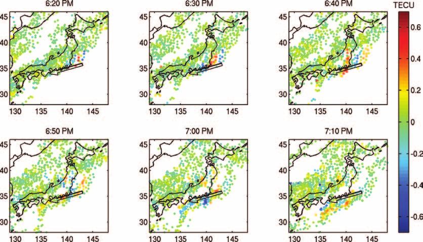
wave was detected on tide gauges in Japan (Fig. 4) with ampli- a cut-off at 30 min. However, this simple data processing may lead
tudes between 10 and 40 cm, 20 to 22 hr after the earthquake. to two errors in the interpretation.
Two dominant frequencies are apparent on the spectrograms, ap-
proximately 0.75 and 0.5 mHz, corresponding to periods of 22 and (i) First, we are now measuring perturbations of the electron con-
33 min. tent which could well be located far below or above the F2 peak. The
C 2005 RAS, GJI, 160, 840–848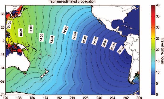
844     J. Artru et al.

                                                                                                                                                         Downloaded from http://gji.oxfordjournals.org/ at California Institute of Technology on November 11, 2014
Figure 4. HNSK (Hanasaki, Hokkaido) Tide gauge time series and spectrogram. The tsunami clearly appears as short-period, small amplitudes fluctuations
compared to the tidal signal. Two frequency peaks are observed, corresponding to 20 and 30 min of period.

error in the correction factor is probably negligible at this level, but      (2–4 am in local time), a perturbation propagating towards the S-SW,
the mislocation of the piercing point can be important, especially for        with a peak-to-peak amplitude of 1 TECU, was detected along the
low elevation rays. This effect can be mitigated in part by focusing          Northeast coast of Honshu. Previous days processing did not show
our study on a single satellite at a time, where the relative location        such perturbations of the ionosphere at that time. Fig. 5 shows such
of the different measurement point is still accurate.                         maps for several times within the window of the tsunami arrival.
   (ii) Secondly, as the piercing points are moving with time due to          The orientation, wavelength and apparent velocity of the signal are
the satellite motion, some sharp static spatial variations in the TEC         at this point consistent with the expected characteristics described
may appear in the time series as short period signal, and therefore           in Section 2.1.
would not be filtered out. Such an aliasing can however be identified
a posteriori by looking at several receivers simultaneously.
                                                                              4 DISCUSSION

3.3 Data processing                                                           4.1 Signal observed
We processed ionospheric data from the Japanese continuous GPS                Let us look at the signal observed in greater detail. Because of the
network (GEONET). This network consists of more than 1000 con-                possible aliasing of spatial variations of TEC into the filtered time
tinuous receivers, and presents a remarkable coverage of the Japan            series, a careful analysis of the geometry of the signal is needed. It
archipelago. Each receiver can usually receive signals from six or            is however possible to take advantage of the high density of the net-
more satellites with a 30 s sampling rate, providing more than                work to mitigate this effect. We isolated the data from one satellite–
6000 TEC measurements at each time. This data set extends 500 to              all receivers and ploted the corresponding time series as functions
800 km offshore when a satellite is seen with a low elevation angle.          of time and distance from the epicentre (Fig. 6). In the ideal case of
   At each time, we plotted the value of the filtered TEC at the              a tsunami propagating at a constant speed, the signals would have
corresponding ionospheric piercing points. Traveling ionospheric              appeared along as straight line corresponding to the tsunami ve-
disturbances can be frequently detected throughout the day, with              locity. Here we find that the signal is indeed consitent with some
amplitudes varying from a fraction to several TEC units, but most             velocity in the range 150–250 m s−1 , which is consistent with our
occur during daytime. At the estimated arrival time of the tsunami            interpretation.


                                                                                                                      C   2005 RAS, GJI, 160, 840–848
Atmospheric gravity waves induced by tsunamis                      845

                                                                                                                                                                      Downloaded from http://gji.oxfordjournals.org/ at California Institute of Technology on November 11, 2014
Figure 5. Observed signal: TEC variations plotted at the ionospheric piercing points. A wave-like disturbance is propagating towards the coast of Honshu.
This perturbation presents the expected characteristics of a tsunami induced gravity waves, and arrives approximately at the same time as the tsunami wave
itself.

Figure 6. Time series for satellite 22 at the time of the tsunami arrival. The left panel shows the TEC variations as a function of time and distance from the
epicentre (along the great circle path). The right panel shows the same time series at the moving location of the ionospheric piercing points (350 km of altitude).


C   2005 RAS, GJI, 160, 840–848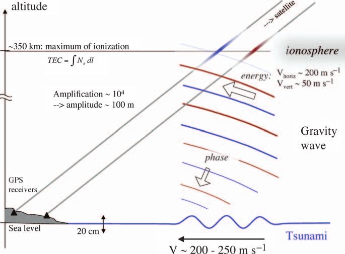
846      J. Artru et al.

                                                                                   shown on Fig. 3 (Koshimura 2004, personnal communication). Us-
                                                                                   ing these travel times, we calculated the arrival time for the tsunami-
                                                                                   induced gravity wave. At each point we calculated the tsunami speed
                                                                                   from the bathymetry. Then we determined the horizontal and ver-
                                                                                   tical group velocities for a 30-min period gravity wave induced
                                                                                   by the tsunami (assuming an isothermal atmosphere in which c =
                                                                                   350 m s−1 ). From these values and from the orientation of the
                                                                                   tsunami wave front, we calculated the position and arrival time of
                                                                                   the gravity wave at 350 km of altitude. The resulting arrival time
                                                                                   map is shown on the middle panel of Fig. 7. We can compare directly
                                                                                   those calculated arrival times with the time picks on the GPS time
                                                                                   series (Fig. 7, lower panel). The agreement is fairly good, although
                                                                                   the observed wave appears to be slower by 20 per cent. This is stil
                                                                                   reasonable considering that the isothermal approximation clearly
                                                                                   does not hold at high altitude.

                                                                                                                                                             Downloaded from http://gji.oxfordjournals.org/ at California Institute of Technology on November 11, 2014
                                                                                   4.3 Number and type of TIDS imaged with this processing
                                                                                   As we mentioned in Section 2.3, TIDs are a very common phe-
                                                                                   nomenon, and it is very hard to determine the origin of such per-
                                                                                   turbations. It is virtually impossible to rule out some other interpre-
                                                                                   tation for the origin of the signal that is the focus of our study. In
                                                                                   order to confirm that the signal observed may indeed be related to the
                                                                                   tsunami, we first checked that no such signal appeared in the preced-
                                                                                   ing and following days. This shows that the wave is most likely not
                                                                                   related to diurnal variations of the ionosphere. We also performed a
                                                                                   simple count of the wave-like perturbations appearing through our
                                                                                   data processing, with amplitudes higher than 0.1 TECU. We noted
                                                                                   their location, time, apparent azimuth and velocity throughout 2001
                                                                                   June 23 and 24. The results are presented on Fig. 8. Amplitudes
                                                                                   observed do not exceed 2.5 TECU, and as expected, daytime iono-
                                                                                   sphere presents much more TIDs than nighttime.

                                                                                   5 C O N C LU S I O N
                                                                                   We presented here an ionospheric perturbation possibly induced by
                                                                                   a tsunami. The detection was made off shore using Japan GEONET
                                                                                   permanent GPS network. The signal observed is in good agreeement
                                                                                   with what is expected from theoretical considerations, and opens
                                                                                   exciting perspectives for the study of tsunamis up to several hundred
                                                                                   kilometres from the coastline. The fundamental features of this study
                                                                                   and observation are as follows.
Figure 7. Tsunami arrival times (GMT) predicted and observed. The top
                                                                                      Tsunami waves are expected to couple with atmospheric gravity
panel is a close-up of Fig. 3 showing tsunami estimated arrival times (at sea      wave. The latter propagates obliquely upwards and interacts with
level) in the area of study. The middle panel shows the result of the arrival      the ionospheric plasma at high altitude. Noise caused by shorter
time estimation, at 350 km of altitude, for the induced gravity wave. The bot-     wavelength sea-level perturbations (ocean swell) is filtered out in
tom panel shows the observed arrival times, obtained by cross-correlation of       the process.
all the time series from satellite 22. These travel times give an apparent hori-      GPS ionospheric monitoring using a dense network is a powerfull
zontal velocity of between 150 and 200 m s−1 . The azimuth is approximately        tool to image small-scale perturbations of the ionosphere over large
250◦ .                                                                             areas, in particular extending several hundred kilometres from the
                                                                                   network location, thanks to oblique satellite-receiver rays.
4.2 Arrival times: observations and simulations
                                                                                      The analysis for the Peru, 2001 June 23 earthquake and tsunami
In a second step, we pick the arrival times of the signal on each of the           showed indeed a signal with the expected characteristics. The sea
time series (by cross-correlation with a reference trace). The bottom              level displacement for this tsunami wave is of the order of 1–2 cm,
panel of Fig. 7 shows the travel times obtained. From these travel                 and the amplitude of the ionospheric perturbation is ±1 TECU. This
times, we can estimate the velocity and azimuth of the perturbation.               amplitude is similar to most of the TIDs observed during that day;
We find a velocity of 150 m s1 (±30 per cent), and an azimuth of                   however, a larger tsunami would be expected to produce ionospheric
250◦ . Both are consistent with a tsunami wave propagating from the                perturbations larger than this background activity.
coast of Peru.                                                                        This is so far a unique observation, that will need to be confirmed
   Tsunami estimated arrival (ETA) times can be calculated from the                both on future tsunami occurences, and through a better understand-
bathymetry. The arrival time map for the 2001 June 23 tsunami is                   ing of the coupling mechanism. In particular several difficulties in


                                                                                                                          C   2005 RAS, GJI, 160, 840–848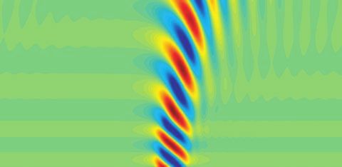
Atmospheric gravity waves induced by tsunamis                     847

                                                 June 24th, 2001
              50˚N

                                                                                                                       24 GMT / 9am LT

              45˚N
                                                                                                                       21 GMT / 6am LT

                                                                                                                       18 GMT / 3am LT
              40˚N
                                                                                                                       15 GMT / 12am LT

                                                                                                                                                                   Downloaded from http://gji.oxfordjournals.org/ at California Institute of Technology on November 11, 2014
                                                                                                                       12 GMT / 9pm LT
              35˚N

                                                                                                                        9 GMT / 6pm LT

              30˚N                                                                                                      6 GMT / 3pm LT

                                                                                                                        3 GMT / 12pm LT
              25˚N

                                                                                                                        0 GMT / 9am LT
                                                                                           100 m s−1
              20˚N
                         125˚E         130˚E        135˚E         140˚E         145˚E        150˚E
Figure 8. Waves observed on filtered TEC maps throughout 2001 June 24. The thickness of the arrows indicate the approximate amplitude of the wave (lower
than 0.75 TECU, between 0.75 and 1.5 TECU, and between 1.5 and 2.25 TECU). The direction is the azimuth, and the lenght is proportional to the speed.
Finally, the colour indicate the time of observation (reddish colours are the local day time, blue is nighttime). The ellipse shows the possible tsunami signal.

the description of the atmospheric–ionospheric perturbation have                   Artru, J., Lognonné, P. & Blanc, E., 2001. Normal modes modelling
to be addressed, e.g. reflection in the atmosphere, attenuation, effi-               of post-seismic ionospheric oscillations, Geophys. Res. Lett., 28(4),
ciency of the gravity wave–ionosphere coupling, dispersion of the                    697–700.
signal. However, the perspectives for this work are very exciting, as              Artru, J., Farges, T. & Lognonné, P., 2004. Acoustic waves generated from
tsunami waves are extremely difficult to observe in the open ocean:                  seismic surface waves: propagation properties determined from Doppler
                                                                                     sounding observation and normal-mode modeling, Geophys. J. Int., 158,
the associated gravity waves in the upper atmosphere might prove
                                                                                     1067–1077 (doi: 10.1111/j.1365-246X.2004.02377.x).
to be a valuable signature.                                                        Blanc, E., 1985. Observations in the upper atmosphere of infrasonic waves
                                                                                     from natural or artificial sources: A summary, Ann. Geophys.,3(6), 673–
                                                                                     688.
AC K N OW L E D G M E N T S
                                                                                   Bolt, B.A., 1964. Seismic air waves from the great 1964 Alaska earthquake,
Caltech contribution number 9104, IPGP 2021. Funding for this                        Nature, 202(4937), 1095–1096.
study was provided by NASA Solid Earth and Natural Hazard Re-                      Calais, E. & Minster, J.B., 1995. GPS detection of ionospheric perturbations
search Program. P. Lognonné and V. Ducic were funded by ESA                         following the January 17, 1994, Northridge earthquake, Geophys. Res.
                                                                                     Lett., 22(9), 1045–1048.
space weather pilot projects. Dr Shunichi Koshimura (DRI, Japan)
                                                                                   Calais, E. & Minster, J.B., 1998. GPS, earthquakes, the ionosphere, and the
provided the tsunami estimated arrival times. We wish to thank Dr                    space shuttle, Phys. Earth planet. Inter., 105, 167–181.
Attila Komjathy (JPL, USA) for help regarding GPS data process-                    Calais, E., Minster, J.B., Hofton, M.A. & Hedlin, M.A.H., 1998. Ionospheric
ing, as well as Professor Toshiro Tanimoto for constructive review.                  signature of surface mine blasts from global positioning system measure-
                                                                                     ments, Geophys. J. Int., 132(1), 191–202.
                                                                                   Clark, R.M., Yeh, K.C. & Liu, C.H., 1971. Interaction of internal gravity
REFERENCES                                                                           waves with the ionospheric f2-layer, Phys. Earth planet. Inter., 33, 1567–
                                                                                     1576.
Artru, J., 2001. Ground-based or satellite observations and modeling of post-      Ducic, V., Artru, J. & Lognonné, P., 2003. Ionospheric remote sensing of the
  seismic ionospheric signals, PhD thesis, Institut de Physique du Globe de          denali earthquake rayleigh surface waves, Geophys. Res. Lett., 30(18),
  Paris (in French).                                                                 1951–1954, doi:10.1029/2003GL017,812.


C   2005 RAS, GJI, 160, 840–848
848 J. Artru et al.
Garcès, M., Hansen, R. & Lindquist, K., 1998. Traveltimes for infrasonic spheric disturbances and 3-m scale irregularitires in the nighttime f-region
waves propagating in a stratified atmosphere, Geophys. J. Int., 135, 255– ionosphere with the mu radar and gps network, Earth Planet Space., 54,
263. 31–44.
Garcès, M., Hetzer, C., Merrifield, M., Willis, M. & Aucan, J., 2003. Ob- Tanioka, Y., 1999. Analysis of the far-field tsunamis generated by the
servations of surf infrasound in Hawai‘i, Geophys. Res. Lett., 30(24), 1998 Papua New Guinea earthquake, Geophys. Res. Lett., 26(22),
2264–2267, doi: 10.1029/2003GL018,614. 3393–3396.
Gonzalez, F.I., Milburn, H.M., Bernard, E.N. & Newman, J.C., 1998. Deep- Virieux, J., Garnier, N., Blanc, E. & Dessa, J.-X., 2004. Paraxial ray tracing
ocean assessment and reporting of tsunamis (dart): Brief overview and for atmospheric wave propagation, Geophys. Res. Lett., 31(20), L20105,
status report, in Proceedings of the International Workshop on Tsunami doi:10.1029/2004 GL 020514.
Disaster Mitigation, 19–22 January 1998, Tokyo, Japan. Yeh, K.C. & Liu, C.H., 1972. Theory of ionospheric waves 402–418 pp.,
Harkrider, D.G., 1964. Theoretical and observed acoustic-gravity waves New York, Academic Press.
from explosive sources in the atmosphere, J. geophys. Res., 69, 5295.
Hatanaka, Y., Iizuka, T., Sawada, M., Yamagiwa, A., Kikuta, Y., John-
son, J.M. & Rocken, C., 2003. Improvement of the analysis strategy of
GEONET, Bull. Geogr. Surv. Inst., 49, 11–37. A P P E N D I X A : A C O U S T I C - G R AV I T Y
Hines, C.O., 1960. Internal atmospheric gravity waves at ionospheric heights,
WAV E S
Canadian J. of Phys., 38, 1441–1481.
Downloaded from http://gji.oxfordjournals.org/ at California Institute of Technology on November 11, 2014
Hino, R., Tanioka, Y., Kanazawa, T., Sakai, S., Nishino, M. & Suyehiro, Hines (1960) established a convenient description of acoustic-
K., 2001. Micro-tsunami from a local interplate earthquake detected by gravity waves in an inviscid, isothermal atmosphere. The equations
cabled offshore tsunami observation in northeastern japan, Geophys. Res. of motion are:
Lett., 28(18), 3533–3536.
∂ρ
International Tsunami Information Center–ITIC, 2001. 23–24 june Continuity : + v · ∇ρ = −ρ∇ · v
2001 20:33 GMT–Peruvian earthquake and tsunami, http://www.prh. ∂t
noaa.gov/itic. ∂v 1
Kanamori, H., Mori, J. & Harkrider, D.G., 1994. Excitation of atmospheric Momentum : + v · ∇v = g − ∇ p
∂t ρ
oscillations by volcanic eruptions, J. geophys. Res., 22, 21947–21961.
Kato, T., Terada, Y., Kinoshita, M., Kakimoto, H., Isshiki, H., Matsuishi, ∂p ∂ρ
Adiabaticity : + v · ∇ p = Cs 2 +v·∇p
M., Yokoyama, A. & Tanno, T., 2000. Real-time observation of tsunami ∂t ∂t
by rtk-gps, Earth Planet Space., 52(10), 841–845.
Kirchengast, G., 1996. Elucidation of the physics of the gravity wave-tid rela-
where ρ is the density, p is the pressure, v is the neutral gas velocity,
tionship with the aid of theoretical simulations, J. geophys. Res., 101(A6), g is the acceleration due to gravity and C s is the constant sound
13 353–13 368. speed. In the equilibrium state, v 0 = 0 and both ρ 0 and p 0 are
Lognonné, P., Clévédé, E. & Kanamori, H., 1998. Computation of seismo- proportional to exp (z/2H), where H = Cs 2 /γ g is the density scale
grams and atmospheric oscillations by normal-mode summation for a height, γ being the specific heat ratio. Assuming ρ 1 , p 1 , and v are
spherical earth model with realistic atmosphere, Geophys. J. Int., 135(2), small perturbations with no dependency along the y-axis, we may
388–406. solve the linearized equations to obtain harmonic solutions with
Mannucci, A.J., 1998. A global mapping technique for gps-derived iono- ρ 1 /ρ 0 , p 1 / p 0 and v proportional to exp[i(ωt − kx x − kz z)]. If we
spheric electron content measurements, Radio Science, 33, 565–582. define k z = kz + i/2H , the following dispersion relation may be
Najita, K., Weaver, P.F. & Yuen, P.C., 1973. A tsunami warning system
derived:
using an ionospheric technique, Proceedings of the IEEE, 62(5), 563–
567.
ω4 − ω2 Cs2 k x2 + k z + (γ − 1)g 2 k x2 − γ 2 g 2 ω2 4Cs2
2
(A1)
Najita, K. & Yuen, P.C., 1979. Long-Period Oceanic Rayleigh Wave Group
Velocity Dispersion Curve From HF Doppler Sounding of the Ionosphere,
Propagating solutions, with k z real, exist for two frequency ranges:
J. geophys. Res., 84(A4), 1253–1260.
acoustic modes (ω > ω a = γ g/2Cs ) are governed primarily by
Okal, E.A., Piatanesi, A. & Heinrich, P., 1999. Tsunami detection by satellite
altimetry, J. geophys. Res., 104(B1), 599–615. compression whereas gravity modes (ω < ω g = γ − 1)1/2 g/Cs )
Peltier, W.R. & Hines, C.O., 1976. On the possible detection of tsunamis by are governed primarily by buoyancy (ω g is the Brunt-Väisälä fre-
a monitoring of the ionosphere, J. geophys. Res., 81(12), 1995–2000. quency). Typically ω a /2π = 3.3 mHz and ω g /2π = 2.9 mHz in
Saito, A., Nishimura, M., Yamamoto, M., Fukao, S., Tsugawa, T., Otsuka, the lower atmosphere. The scale height H drives the exponential
Y., Miyazaki, S. & Kelley, M.C., 2002. Observations of traveling iono- increase of the amplitude with altitude.
C 2005 RAS, GJI, 160, 840–848You can also read