ROS Navigation Tuning Guide
←
→
Page content transcription
If your browser does not render page correctly, please read the page content below

ROS Navigation Tuning Guide
                                                                                Kaiyu Zheng
                                                                            September 2, 2016∗
arXiv:1706.09068v2 [cs.RO] 8 Apr 2019

                                        Abstract
                                        The ROS navigation stack is powerful for mobile robots to move from place to place
                                        reliably. The job of navigation stack is to produce a safe path for the robot to execute,
                                        by processing data from odometry, sensors and environment map. Maximizing the
                                        performance of this navigation stack requires some fine tuning of parameters, and this
                                        is not as simple as it looks. One who is sophomoric about the concepts and reasoning
                                        may try things randomly, and wastes a lot of time.
                                            This article intends to guide the reader through the process of fine tuning naviga-
                                        tion parameters. It is the reference when someone need to know the ”how” and ”why”
                                        when setting the value of key parameters. This guide assumes that the reader has
                                        already set up the navigation stack and ready to optimize it. This is also a summary
                                        of my work with the ROS navigation stack.

                                        Topics
                                          1. Velocity and Acceleration                                 ii. DWA forward simulation
                                                                                                      iii. DWA trajectory scoring
                                          2. Global Planner
                                                                                                      iv. Other DWA parameters
                                                 (a) Global Planner Selection
                                                                                             4. Costmap Parameters
                                                 (b) Global Planner Parameters
                                                                                             5. AMCL
                                          3. Local Planner
                                                                                             6. Recovery Behavior
                                                 (a) Local Planner Selection
                                                 (b) DWA Local Planner                       7. Dynamic Reconfigure

                                                        i. DWA algorithm                     8. Problems
                                          ∗
                                              Update on April 8th, 2019 (added information on amcl)

                                                                                        1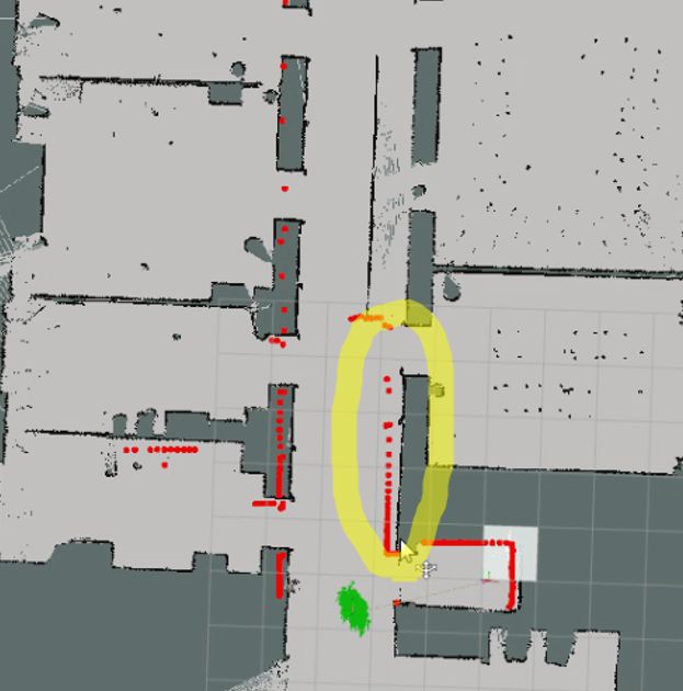
1         Velocity and Acceleration
This section concerns with synchro-drive robots. The dynamics (e.g. velocity and
acceleration of the robot) of the robot is essential for local planners including dy-
namic window approach (DWA) and timed elastic band (TEB). In ROS navigation
stack, local planner takes in odometry messages (”odom” topic) and outputs velocity
commands (”cmd vel” topic) that controls the robot’s motion.

Max/min velocity and acceleration are two basic parameters for the mobile base.
Setting them correctly is very helpful for optimal local planner behavior. In ROS
navigation, we need to know translational and rotational velocity and acceleration.

1.1       To obtain maximum velocity
Usually you can refer to your mobile base’s manual. For example, SCITOS G5 has
maximum velocity 1.4 m/s1 . In ROS, you can also subscribe to the odom topic to
obtain the current odometry information. If you can control your robot manually
(e.g. with a joystick), you can try to run it forward until its speed reaches constant,
and then echo the odometry data.
    Translational velocity (m/s) is the velocity when robot is moving in a straight line.
Its max value is the same as the maximum velocity we obtained above. Rotational
velocity (rad/s) is equivalent as angular velocity; its maximum value is the angular
velocity of the robot when it is rotating in place. To obtain maximum rotational
velocity, we can control the robot by a joystick and rotate the robot 360 degrees after
the robot’s speed reaches constant, and time this movement.
    For safety, we prefer to set maximum translational and rotational velocities to be
lower than their actual maximum values.

1.2       To obtain maximum acceleration
There are many ways to measure maximum acceleration of your mobile base, if your
manual does not tell you directly.
    In ROS, again we can echo odometry data which include time stamps, and them
see how long it took the robot to reach constant maximum translational velocity (ti ).
Then we use the position and velocity information from odometry (nav msgs/Odometry
message) to compute the acceleration in this process. Do several trails and take the
average. Use tt , tr to denote the time used to reach translationand and rotational
maximum velocity from static, respectively. The maximum translational acceleration
at,max = max dv/dt ≈ vmax /tt . Likewise, rotational acceleration can be computed by
ar,max = max dω/dt ≈ ωmax /tr .
    1
        This information is obtained from MetraLabs’s website.

                                                   2
1.3     Setting minimum values
Setting minimum velocity is not as formulaic as above. For minimum translational
velocity, we want to set it to a large negative value because this enables the robot
to back off when it needs to unstuck itself, but it should prefer moving forward in
most cases. For minimum rotational velocity, we also want to set it to negative (if
the parameter allows) so that the robot can rotate in either directions. Notice that
DWA Local Planner takes the absolute value of robot’s minimum rotational velocity.

1.4     Velocity in x, y direction
x velocity means the velocity in the direction parallel to robot’s straight move-
ment. It is the same as translational velocity. y velocity is the velocity in the
direction perpendicular to that straight movement. It is called ”strafing velocity” in
teb local planner. y velocity should be set to zero for non-holonomic robot (such
as differential wheeled robots).

2       Global Planner
2.1     Global Planner Selection
To use the move base node in navigation stack, we need to have a global planner and a
local planner. There are three global planners that adhere to nav core::BaseGlobal
Planner interface: carrot planner, navfn and global planner.

2.1.1    carrot planner

This is the simplest one. It checks if the given goal is an obstacle, and if so it picks an
alternative goal close to the original one, by moving back along the vector between
the robot and the goal point. Eventually it passes this valid goal as a plan to the
local planner or controller (internally). Therefore, this planner does not do any global
path planning. It is helpful if you require your robot to move close to the given goal
even if the goal is unreachable. In complicated indoor environments, this planner is
not very practical.

2.1.2    navfn and global planner

navfn uses Dijkstra’s algorithm to find a global path with minimum cost between
start point and end point. global planner is built as a more flexible replacement
of navfn with more options. These options include (1) support for A∗, (2) toggling
quadratic approximation, (3) toggling grid path. Both navfn and global planner are
based on the work by [Brock and Khatib, 1999]:

                                            3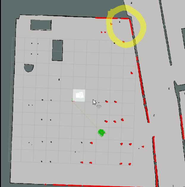
2.2     Global Planner Parameters
Since global planner is generally the one that we prefer, let us look at some of its
key parameters. Note: not all of these parameters are listed on ROS’s website, but
you can see them if you run the rqt dynamic reconfigure program: with
                         rosrun rqt reconfigure rqt reconfigure
   We can leave allow unknown(true), use dijkstra(true), use quadratic(true),
use grid path(false), old navfn behavior(false) to their default values. Setting
visualize potential(false) to true is helpful when we would like to visualize the
potential map in RVIZ.

              Figure 1: Dijkstra path                                Figure 2: A* path

           Figure 3: Standard Behavior                              Figure 4: Grid Path

   Besides these parameters, there are three other unlisted parameters that ac-
tually determine the quality of the planned global path. They are cost factor,
neutral cost, lethal cost. Actually, these parameters also present in navfn. The
source code2 has one paragraph explaining how navfn computes cost values.
  2
      https://github.com/ros-planning/navigation/blob/indigo-devel/navfn/include/navfn/navfn.h

                                                   4
Figure 5: cost factor = 0.01
                               Figure 6: cost factor = 0.55   Figure 7: cost factor = 3.55

Figure 8: neutral cost = 1                                    Figure 10: neutral cost = 233

                               Figure 9: neutral cost = 66

                                            5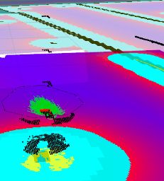
navfn cost values are set to

            cost = COST NEUTRAL + COST FACTOR * costmap cost value.
      Incoming costmap cost values are in the range 0 to 252. The comment also says:

        With COST NEUTRAL of 50, the COST FACTOR needs to be about 0.8 to
        ensure the input values are spread evenly over the output range, 50 to
        253. If COST FACTOR is higher, cost values will have a plateau around
        obstacles and the planner will then treat (for example) the whole width
        of a narrow hallway as equally undesirable and thus will not plan paths
        down the center.

Experiment observations Experiments have confirmed this explanation. Setting
cost factor to too low or too high lowers the quality of the paths. These paths do
not go through the middle of obstacles on each side and have relatively flat curvature.
Extreme neutral cost values have the same effect. For lethal cost, setting it to
a low value may result in failure to produce any path, even when a feasible path is
obvious. Figures 5 − 10 show the effect of cost factor and neutral cost on global
path planning. The green line is the global path produced by global planner.
    After a few experiments we observed that when cost factor = 0.55, neutral cost
= 66, and lethal cost = 253, the global path is quite desirable.

3       Local Planner Selection
Local planners that adhere to nav core::BaseLocalPlanner interface are dwa local
 planner, eband local planner and teb local planner. They use different al-
gorithms to generate velocity commands. Usually dwa local planner is the go-to
choice. We will discuss it in detail. More information on other planners will be
provided later.

3.1     DWA Local Planner
3.1.1     DWA algorithm

See next page.

                                          6
dwa local planner uses Dynamic Window Approach (DWA) algorithm. ROS
Wiki provides a summary of its implementation of this algorithm:
1. Discretely sample in the robot’s control space (dx,dy,dtheta)
2. For each sampled velocity, perform forward simulation from the robot’s
current state to predict what would happen if the sampled velocity were
applied for some (short) period of time.
3. Evaluate (score) each trajectory resulting from the forward simulation,
using a metric that incorporates characteristics such as: proximity to
obstacles, proximity to the goal, proximity to the global path, and
speed. Discard illegal trajectories (those that collide with obstacles).
4. Pick the highest-scoring trajectory and send the associated velocity to
the mobile base.
5. Rinse and repeat.
DWA is proposed by [Fox et al., 1997]. According to this paper, the goal of DWA
is to produce a (v, ω) pair which represents a circular trajectory that is optimal for
robot’s local condition. DWA reaches this goal by searching the velocity space in
the next time interval. The velocities in this space are restricted to be admissible,
which means the robot must be able to stop before reaching the closest obstacle on
the circular trajectory dictated by these admissible velocities. Also, DWA will only
consider velocities within a dynamic window, which is defined to be the set of velocity
pairs that is reachable within the next time interval given the current translational
and rotational velocities and accelerations. DWA maximizes an objective function
that depends on (1) the progress to the target, (2) clearance from obstacles, and (3)
forward velocity to produce the optimal velocity pair.
Now, let us look at the algorithm summary on ROS Wiki. The first step is to
sample velocity pairs (vx , vy , ω) in the velocity space within the dynamic window.
The second step is basically obliterating velocities (i.e. kill off bad trajectories) that
are not admissible. The third step is to evaluate the velocity pairs using the objec-
tive function, which outputs trajectory score. The fourth and fifth steps are easy to
understand: take the current best velocity option and recompute.
This DWA planner depends on the local costmap which provides obstacle infor-
mation. Therefore, tuning the parameters for the local costmap is crucial for optimal
behavior of DWA local planner. Next, we will look at parameters in forward simula-
tion, trajectory scoring, costmap, and so on.
73.1.2 DWA Local Planner : Forward Simulation
Forward simulation is the second step of the DWA algorithm. In this step, the
local planner takes the velocity samples in robot’s control space, and examine the
circular trajectories represented by those velocity samples, and finally eliminate bad
velocities (ones whose trajectory intersects with an obstacle). Each velocity sample
is simulated as if it is applied to the robot for a set time interval, controlled by
sim time(s) parameter. We can think of sim time as the time allowed for the robot
to move with the sampled velocities.
Through experiments, we observed that the longer the value of sim time, the
heavier the computation load becomes. Also, when sim time gets longer, the path
produced by the local planner is longer as well, which is reasonable. Here are some
suggestions on how to tune this sim time parameter.
How to tune sim time Setting sim time to a very low value (= 5.0) will result in long curves that are not very flexible. This
problem is not that unavoidable, because the planner actively replans after each time
interval (controlled by controller frequency(Hz)), which leaves room for small
adjustments. A value of 4.0 seconds should be enough even for high performance
computers.
Figure 11: sim time = 1.5 Figure 12: sim time = 4.0
Besides sim time, there are several other parameters that worth our attention.
8Velocity samples Among other parameters, vx sample, vy sample determine how
many translational velocity samples to take in x, y direction. vth sample controls
the number of rotational velocities samples. The number of samples you would like
to take depends on how much computation power you have. In most cases we prefer
to set vth samples to be higher than translational velocity samples, because turning
is generally a more complicated condition than moving straight ahead. If you set
max vel y to be zero, there is no need to have velocity samples in y direction since
there will be no usable samples. We picked vx sample = 20, and vth samples = 40.
Simulation granularity sim granularity is the step size to take between points
on a trajectory. It basically means how frequent should the points on this trajectory
be examined (test if they intersect with any obstacle or not). A lower value means
higher frequency, which requires more computation power. The default value of 0.025
is generally enough for turtlebot-sized mobile base.
3.1.3 DWA Local Planner : Trajactory Scoring
As we mentioned above, DWA Local Planner maximizes an objective function to
obtain optimal velocity pairs. In its paper, the value of this objective function relies
on three components: progress to goal, clearance from obstacles and forward velocity.
In ROS’s implementation, the cost of the objective function is calculated like this:
cost = path distance bias ∗ (distance(m) to path from the endpoint of the trajectory)
+ goal distance bias ∗ (distance(m) to local goal from the endpoint of the trajectory)
+ occdist scale ∗ (maximum obstacle cost along the trajectory in obstacle cost (0-254))
The objective is to get the lowest cost. path distance bias is the weight for how
much the local planner should stay close to the global path [Furrer et al., 2016]. A
high value will make the local planner prefer trajectories on global path.
goal distance bias is the weight for how much the robot should attempt to
reach the local goal, with whatever path. Experiments show that increasing this
parameter enables the robot to be less attached to the global path.
occdist scale is the weight for how much the robot should attempt to avoid ob-
stacles. A high value for this parameter results in indecisive robot that stucks in place.
Currently for SCITOS G5, we set path distance bias to 32.0, goal distance bias
to 20.0, occdist scale to 0.02. They work well in simulation.
93.1.4 DWA Local Planner : Other Parameters
Goal distance tolerance These parameters are straightforward to understand.
Here we will list their description shown on ROS Wiki:
• yaw goal tolerance (double, default: 0.05) The tolerance in radians for the
controller in yaw/rotation when achieving its goal.
• xy goal tolerance (double, default: 0.10) The tolerance in meters for the
controller in the x & y distance when achieving a goal.
• latch xy goal tolerance (bool, default: false) If goal tolerance is latched, if
the robot ever reaches the goal xy location it will simply rotate in place, even
if it ends up outside the goal tolerance while it is doing so.
Oscilation reset In situations such as passing a doorway, the robot may oscilate
back and forth because its local planner is producing paths leading to two opposite
directions. If the robot keeps oscilating, the navigation stack will let the robot try its
recovery behaviors.
• oscillation reset dist (double, default: 0.05) How far the robot must travel
in meters before oscillation flags are reset.
4 Costmap Parameters
As mentioned above, costmap parameters tuning is essential for the success of local
planners (not only for DWA). In ROS, costmap is composed of static map layer,
obstacle map layer and inflation layer. Static map layer directly interprets the given
static SLAM map provided to the navigation stack. Obstacle map layer includes 2D
obstacles and 3D obstacles (voxel layer). Inflation layer is where obstacles are inflated
to calculate cost for each 2D costmap cell.
Besides, there is a global costmap, as well as a local costmap. Global costmap is
generated by inflating the obstacles on the map provided to the navigation stack.
Local costmap is generated by inflating obstacles detected by the robot’s sensors in
real time.
There are a number of important parameters that should be set as good as possible.
4.1 footprint
Footprint is the contour of the mobile base. In ROS, it is represented by a two
dimensional array of the form [x0 , y0 ], [x1 , y1 ], [x2 , y2 ], ...], no need to repeat the first
coordinate. This footprint will be used to compute the radius of inscribed circle and
10Figure 13: inflation decay
circumscribed circle, which are used to inflate obstacles in a way that fits this robot.
Usually for safety, we want to have the footprint to be slightly larger than the robot’s
real contour.
To determine the footprint of a robot, the most straightforward way is to refer
to the drawings of your robot. Besides, you can manually take a picture of the top
view of its base. Then use CAD software (such as Solidworks) to scale the image
appropriately and move your mouse around the contour of the base and read its
coordinate. The origin of the coordinates should be the center of the robot. Or, you
can move your robot on a piece of large paper, then draw the contour of the base.
Then pick some vertices and use rulers to figure out their coordinates.
4.2 inflation
Inflation layer is consisted of cells with cost ranging from 0 to 255. Each cell is either
occupied, free of obstacles, or unknown. Figure 13 shows a diagram 3 illustrating how
inflation decay curve is computed.
inflation radius and cost scaling factor are the parameters that determine
the inflation. inflation radius controls how far away the zero cost point is from
3
Diagram is from http://wiki.ros.org/costmap_2d
11the obstacle. cost scaling factor is inversely proportional to the cost of a cell.
Setting it higher will make the decay curve more steep.
Dr. Pronobis sugggests the optimal costmap decay curve is one that has rel-
atively low slope, so that the best path is as far as possible from the obstacles
on each side. The advantage is that the robot would prefer to move in the mid-
dle of obstacles. As shown in Figure 8 and 9, with the same starting point and
goal, when costmap curve is steep, the robot tends to be close to obstacles. In
Figure 14, inflation radius = 0.55, cost scaling factor = 5.0; In Figure 15,
inflation radius = 1.75, cost scaling factor = 2.58
Figure 14: steep inflation curve
Figure 15: gentle inflation curve
Based on the decay curve diagram, we want to set these two parameters such
that the inflation radius almost covers the corriders, and the decay of cost value is
moderate, which means decrease the value of cost scaling factor .
4.3 costmap resolution
This parameter can be set separately for local costmap and global costmap. They
affect computation load and path planning. With low resolution (>= 0.05), in narrow
passways, the obstacle region may overlap and thus the local planner will not be able
to find a path through.
For global costmap resolution, it is enough to keep it the same as the resolution
of the map provided to navigation stack. If you have more than enough computation
power, you should take a look at the resolution of your laser scanner, because when
creating the map using gmapping, if the laser scanner has lower resolution than your
desired map resolution, there will be a lot of small ”unknown dots” because the laser
scanner cannot cover that area, as in Figure 10.
12Figure 16: gmapping resolution = 0.01. Notice the unknown
dots on the right side of the image
For example, Hokuyo URG-04LX-UG01 laser scanner has metric resolution of
0.01mm4 . Therefore, scanning a map with resolution• KinectFusion: Real-time 3D Reconstruction and Interaction Using a Moving
Depth Camera
• Real-time 3D Reconstruction at Scale using Voxel Hashing
voxel grid is a ROS package which provides an implementation of efficient 3D
voxel grid data structure that stores voxels with three states: marked, free, unknown.
The voxel grid occupies the volume within the costmap region. During each update
of the voxel layer’s boundary, the voxel layer will mark or remove some of the voxels
in the voxel grid based on observations from sensors. It also performs ray tracing,
which is discussed next. Note that the voxel grid is not recreated when updating, but
only updated unless the size of local costmap is changed.
Why ray tracing in obstacle layer and voxel layer? Ray tracing is best known
for rendering realistic 3D graphics, so it might be confusing why it is used in dealing
with obstacles. One big reason is that obstacles of different type can be detected by
robot’s sensors. Take a look at figure 17. In theory, we are also able to know if an
obstacle is rigid or soft (e.g. grass)5 .
Figure 17: With ray tracing, laser scanners is able to recognize different types of obstacles.
A good blog on voxel ray tracing versus polygong ray tracing: http://raytracey.
blogspot.com/2008/08/voxel-ray-tracing-vs-polygon-ray.html
With the above understanding, let us look into the parameters for the obstacle
layer6 . These parameters are global filtering parameters that apply to all sensors.
• max obstacle height: The maximum height of any obstacle to be inserted into
the costmap in meters. This parameter should be set to be slightly higher than
the height of your robot. For voxel layer, this is basically the height of the voxel
grid.
5
mentioned in Using Robots in Hazardous Environments by Boudoin, Habib, pp.370
6
Some explanations are directly copied from costmap2d ROS Wiki
14• obstacle range: The default maximum distance from the robot at which an
obstacle will be inserted into the cost map in meters. This can be over-ridden
on a per-sensor basis.
• raytrace range: The default range in meters at which to raytrace out obstacles
from the map using sensor data. This can be over-ridden on a per-sensor basis.
These parameters are only used for the voxel layer (VoxelCostmapPlugin).
• origin z: The z origin of the map in meters.
• z resolution: The z resolution of the map in meters/cell.
• z voxels: The number of voxels to in each vertical column, the height of the
grid is z resolution * z voxels.
• unknown threshold: The number of unknown cells allowed in a column con-
sidered to be ”known”
• mark threshold: The maximum number of marked cells allowed in a column
considered to be ”free”.
Experiment observations Experiments further clarify the effects of the voxel
layer’s parameters. We use ASUS Xtion Pro as our depth sensor. We found that
position of Xtion matters in that it determines the range of ”blind field”, which is
the region that the depth sensor cannot see anything.
In addition, voxels representing obstacles only update (marked or cleared) when
obstacles appear within Xtion range. Otherwise, some voxel information will remain,
and their influence on costmap inflation remains.
Besides, z resolution controls how dense the voxels is on the z-axis. If it is
higher, the voxel layers are denser. If the value is too low (e.g. 0.01), all the voxels
will be put together and thus you won’t get useful costmap information. If you set
z resolution to a higher value, your intention should be to obtain obstacles better,
therefore you need to increase z voxels parameter which controls how many voxels
in each vertical column. It is also useless if you have too many voxels in a column
but not enough resolution, because each vertical column has a limit in height. Figure
18-20 shows comparison between different voxel layer parameters setting.
15Figure 18: Scene: Plant in front Figure 19: high z resolution Figure 20: low z resolution
of the robot
5 AMCL
amcl is a ROS package that deals with robot localization. It is the abbreviation of
Adaptive Monte Carlo Localization (AMCL), also known as partical filter localiza-
tion. This localization technique works like this: Each sample stores a position and
orientation data representing the robot’s pose. Particles are all sampled randomly
initially. When the robot moves, particles are resampled based on their current state
as well as robot’s action using recursive Bayesian estimation.
More discussion on AMCL parameter tuning will be provided later. Please refer
to http://wiki.ros.org/amcl for more information. For the details of the original
algorithm Monte Carlo Localization (MCL), read Chapter 8 of Probabilistic Robotics
[Thrun et al., 2005].
We now summarize several issues that may affect the quality of AMCL localization7 .
We hope this information makes this guide more complete, and you find it useful.
Through experiments, we observed three issues that affect the localization with
AMCL. As described in [Thrun et al., 2005], MCL maintains two probabilistic mod-
els, a motion model and a measurement model. In ROS amcl, the motion model
corresponds to a model of the odometry, while the measurement model correspond
to a model of laser scans. With this general understanding, we describe three issues
separately as follows.
7
Added on April 8th, 2019. This investigation was done in May, 2017, yet not reported in this
guide at the time.
16Figure 21: When LaserScan fields are not correct Figure 22: When LaserScan fields are correct
5.1 Header in LaserScan messages
Messages that are published to scan topic are of type sensor msgs/LaserScan8 . This
message contains a header with fields dependent on the specific laser scanner that you
are using. These fields include (copied from the message documentation)
• angle min (float32) start angle of the scan [rad]
• angle max (float32) end angle of the scan [rad]
• angle increment (float32) start angle of the scan [rad]
• time increment (float32) time between measurements [seconds] - if your scan-
ner is moving, this will be used in interpolating position of 3d points
• scan time (float32) time between scans [seconds]
• range min (float32) minimum range value [m]
• range max (float32) maximum range value [m]
We observed in our experiments that if these values are not set correctly for
the laser scanner product on board, the quality of localization will be affected (see
Figure 21 and 22. We have used two laser scanners products, the SICK LMS 200 and
the SICK LMS 291. We provide their parameters below9 .
8
See: http://docs.ros.org/melodic/api/sensor_msgs/html/msg/LaserScan.html
9
For LMS 200, thanks to this Github issue (https://github.com/smichaud/lidar-snowfall/
issues/1)
17SICK LMS 200:
1 {
2 "range_min": 0.0,
3 "range_max": 81.0,
4 "angle_min": -1.57079637051,
5 "angle_max": 1.57079637051,
6 "angle_increment": 0.0174532923847,
7 "time_increment": 3.70370362361e-05,
8 "scan_time": 0.0133333336562
9 }
SICK LMS 291:
1 {
2 "range_min": 0.0,
3 "range_max": 81.0,
4 "angle_min": -1.57079637051,
5 "angle_max": 1.57079637051,
6 "angle_increment": 0.00872664619235,
7 "time_increment": 7.40740724722e-05,
8 "scan_time": 0.0133333336562
9 }
5.2 Parameters for measurement and motion models
There are parameters listed in the amcl package about tuning the laser scanner model
(measurement) and odometry model (motion). Refer to the package page for the
complete list and their definitions. A detailed discussion requires great understanding
of the MCL algorithm in [Thrun et al., 2005], which we omit here. We provide an
example of fine tuning these parameters and describe their results qualitatively. The
actual parameters you use should depend on your laser scanner and robot.
For laser scanner model, the default parameters are:
1 {
2 "laser_z_hit": 0.5,
3 "laser_sigma_hit": 0.2,
4 "laser_z_rand" :0.5,
5 "laser_likelihood_max_dist": 2.0
6 }
To improve the localization of our robot, we increased laser z hit and laser sigma hit
to incorporate higher measurement noise. The resulting parameters are:
18Figure 23: Default measurement model parame- Figure 24: After tuning measurement model pa-
ters rameters (increase noise)
1 {
2 "laser_z_hit": 0.9,
3 "laser_sigma_hit": 0.1,
4 "laser_z_rand" :0.5,
5 "laser_likelihood_max_dist": 4.0
6 }
The behavior is illustrated in Figure 23 and 24. It is clear that in our case, adding
noise into the measurement model helped with localization.
For the odometry model, we found that our odometry was quite reliable in
terms of stability. Therefore, we tuned the parameters so that the algorithm assumes
there is low noise in odometry:
1 {
2 "kld_err": 0.01,
3 "kld_z": 0.99,
4 "odom_alpha1": 0.005,
5 "odom_alpha2": 0.005,
6 "odom_alpha3": 0.005,
7 "odom_alpha4": 0.005
8 }
To verify that the above paremeters for motion model work, we also tried a set of
19parameters that suggest a noisy odometry model:
1 {
2 "kld_err": 0.10,
3 "kld_z": 0.5’,
4 "odom_alpha1": 0.008,
5 "odom_alpha2": 0.040,
6 "odom_alpha3": 0.004,
7 "odom_alpha4": 0.025
8 }
We observed that when the odometry model is less noisy, the particles are more
condensed. Otherwise, the particles are more spread-out.
5.3 Translation of the laser scanner
There is a tf transform from laser link to base footprint or base link that
indicates the pose of the laser scanner with respect to the robot base. If this transform
is not correct, it is very likely that the localization behaves strangely. In this situation,
we have observed constant shifting of laser readings from the walls of the environment,
and sudden drastic change in the localization. It is straightforward enough to make
sure the transform is correct; This is usually handled in urdf and srdf specification
of your robot. However, if you are using a rosbag file, you may have to publish the
transform youself.
6 Recovery Behaviors
An annoying thing about robot navigation is that the robot may get stuck. Fortu-
nately, the navigation stack has recovery behaviors built-in. Even so, sometimes the
robot will exhaust all available recovery behaviors and stay still. Therefore, we may
need to figure out a more robust solution.
Types of recovery behaviors ROS navigation has two recovery behaviors. They
are clear costmap recovery and rotate recovery. Clear costmap recovery is ba-
sically reverting the local costmap to have the same state as the global costmap.
Rotate recovery is to recover by rotating 360 degrees in place.
Unstuck the robot Sometimes rotate recovery will fail to execute due to rotation
failure. At this point, the robot may just give up because it has tried all of its
recovery behaviors - clear costmap and rotation. In most experiments we observed
that when the robot gives up, there are actually many ways to unstuck the robot. To
avoid giving up, we used SMACH to continuously try different recovery behaviors,
20with additional ones such as setting a temporary goal that is very close to the robot,
and returning to some previously visited pose (i.e. backing off). These methods turn
out to improve the robot’s durability substantially, and unstuck it from previously
hopeless tight spaces from our experiment observations10 .
Figure 25: Simple recovery state in SMACH
Parameters The parameters for ROS’s recovery behavior can be left as default in
general. For clear costmap recovery, if you have a relatively high sim time, which
means the trajectory is long, you may want to consider increasing reset distance
parameter, so that bigger area on local costmap is removed, and there is a better
chance for the local planner to find a path.
7 Dynamic Reconfigure
One of the most flexible aspect about ROS navigation is dynamic reconfiguration,
since different parameter setup might be more helpful for certain situations, e.g.
10
Here is a video demo of my work on mobile robot navigation: https://youtu.be/1-7GNtR6gVk
21when robot is close to the goal. Yet, it is not necessary to do a lot of dynamic
reconfiguration.
Example One situation that we observed in our experiments is that the robot tends
to fall off the global path, even when it is not necessary or bad to do so. Therefore
we increased path distance bias. Since a high path distance bias will make the
robot stick to the global path, which does not actually lead to the final goal due
to tolerance, we need a way to let the robot reach the goal with no hesitation. We
chose to dynamically decrease the path distance bias so that goal distance bias
is emphasized when the robot is close to the goal. After all, doing more experiments
is the ultimate way to find problems and figure out solutions.
8 Problems
1. Getting stuck
This is a problem that we face a lot when using ROS navigation. In both
simulation and reality, the robot gets stuck and gives up the goal.
2. Different speed in different directions
We observed some weird behavior of the navigation stack. When the goal is set
in the -x direction with respect to TF origin, dwa local planner plans less stably
(the local planned trajectory jumps around) and the robot moves really slowly.
But when the goal is set in the +x direction, dwa local planner is much more
stable, and the robot can move faster.
I reported this issue on Github here: https://github.com/ros-planning/
navigation/issues/503. Nobody attempted to resolve it yet.
3. Reality VS. simulation
There is a difference between reality and simulation. In reality, there are more
obstacles with various shapes. For exmaple, in the lab there is a vertical stick
that is used to hold to door open. Because it is too thin, the robot sometimes
fails to detect it and hit on it. There are also more complicated human activity
in reality.
4. Inconsistency
Robots using ROS navigation stack can exhibit inconsistent behaviors, for ex-
ample when entering a door, the local costmap is generated again and again
with slight difference each time, and this may affect path planning, especially
when resolution is low. Also, there is no memory for the robot. It does not
remember how it entered the room from the door the last time. So it needs to
22start out fresh again every time it tries to enter a door. Thus, if it enters the
door in a different angle than before, it may just get stuck and give up.
Thanks
Hope this guide is helpful. Please feel free to add more information from your own
experimental observations.
References
[Brock and Khatib, 1999] Brock, O. and Khatib, O. (1999). High-speed navigation
using the global dynamic window approach. In Proceedings 1999 IEEE Interna-
tional Conference on Robotics and Automation (Cat. No. 99CH36288C), volume 1,
pages 341–346. IEEE.
[Fox et al., 1997] Fox, D., Burgard, W., and Thrun, S. (1997). The dynamic window
approach to collision avoidance. IEEE Robotics & Automation Magazine, 4(1):23–
33.
[Furrer et al., 2016] Furrer, F., Burri, M., Achtelik, M., , and Siegwart, R. (2016).
Robot operating system (ros): The complete reference (volume 1). by A. Koubaa.
Cham: Springer International Publishing.
[Thrun et al., 2005] Thrun, S., Burgard, W., and Fox, D. (2005). Probabilistic
robotics. MIT press.
23You can also read