A Novel Hybrid Deep Learning Model for Sugar Price Forecasting Based on Time Series Decomposition

Hindawi
Mathematical Problems in Engineering
Volume 2021, Article ID 6507688, 9 pages
https://doi.org/10.1155/2021/6507688

Research Article
A Novel Hybrid Deep Learning Model for Sugar Price Forecasting
Based on Time Series Decomposition

 Jinlai Zhang,1 Yanmei Meng ,1 Jin Wei,1 Jie Chen,1 and Johnny Qin2
 1
 College of Mechanical Engineering, Guangxi University, Nanning 530004, China
 2
 Energy, Commonwealth Scientific and Industrial Research Organisation, 1 Technology Court, Pullenvale QLD4069, Australia

 Correspondence should be addressed to Yanmei Meng; gxu_mengyun@163.com

 Received 27 June 2021; Revised 21 July 2021; Accepted 28 July 2021; Published 3 August 2021

 Academic Editor: Francesco Lolli

 Copyright © 2021 Jinlai Zhang et al. This is an open access article distributed under the Creative Commons Attribution License,
 which permits unrestricted use, distribution, and reproduction in any medium, provided the original work is properly cited.
 Sugar price forecasting has attracted extensive attention from policymakers due to its significant impact on people’s daily lives and
 markets. In this paper, we present a novel hybrid deep learning model that utilizes the merit of a time series decomposition
 technology empirical mode decomposition (EMD) and a hyperparameter optimization algorithm Tree of Parzen Estimators
 (TPEs) for sugar price forecasting. The effectiveness of the proposed model was implemented in a case study with the price of
 London Sugar Futures. Two experiments are conducted to verify the superiority of the EMD and TPE. Moreover, the specific
 effects of EMD and TPE are analyzed by the DM test and improvement percentage. Finally, empirical results demonstrate that the
 proposed hybrid model outperforms other models.

1. Introduction forecasting. However, one limitation of abovementioned
 three methods is they do not optimize the hyperparameter of
Sugar is an important food commodity around the world, neural networks. Hyperparameter optimization is a com-
and the fluctuations of food prices have a huge impact on monly used strategy in machine learning area [8] especially
people’s daily lives due to its impact on overall inflation in time series forecasting [3] to improve the performance of
dynamics of many countries [1, 2]. Therefore, it is essential to machine learning models. This is largely due to the explosion
forecast the sugar price accurately. in the field of machine learning in recent years [9] and makes
 Forecasting of sugar prices has attracted a lot interest of some very common technologies appeared in recent years in
researchers for several decades, and it can be divided into the field of machine learning, such as SGD [10], and Adam
statistical methods and machine learning methods. The [11] are proposed after the year of 2014, while most sugar
statistical methods have the advantages of low complexity price forecasting literatures are published before 2014. On
and fast calculation speed [3]. In 1975, Meyer and Kim [4] the other hand, the nonstationarity and nonlinearity of sugar
applied the autoregressive integrated moving average prices [12] make it harder to accurately predict the future
(ARIMA) method in sugar price forecasting. However, the sugar price. In order to handle nonstationarity features, the
ARIMA requires the time series data to be stable or stable inputs for machine learning models need to be properly
after being differentiated, which might limit the application preprocessed [13]. Therefore, some multiresolution analysis
of this method. In 2009, Xu et al. [5] used a neural network techniques are widely used in many forecasting problems
with multiple fully connected layers for sugar price fore- [14, 15]. Conventionally, the discrete wavelet transformation
casting using a Chinese database. In 2011, Ribeiro and (DWT) was used [16, 17]. Hajiabotorabi et al. [18] improved
Oliveira [6] introduced a hybrid model built upon artificial the recurrent neural network (RNN) with the multi-
neural networks (ANNs) and Kalman filter. In 2019, Silva1 resolution based on B-spline wavelet produced by an effi-
et al. [7] investigated ANNs, extreme learning machines cient DWT. Yong and Awang [19] used DWT for improving
(ELMs), and echo state networks (ESNs) for sugar price the forecast accuracy. However, the DWT generally requires

2 Mathematical Problems in Engineering

a lengthy trial and error process [20]. Moreover, the em- ft � σ wf · ht−1 , xt + bf , (1)
pirical mode decomposition [21] (EMD) multiresolution
technique is introduced to time series, which provides self-
 it � σ wi · ht−1 , xt + bi , (2)
adaptability. EMD extracts the salient features via the
temporal local decomposition method and isolates these
significant features into subseries that represent the physical gt � tanh wg · ht−1 , xt + bg , (3)
structure of the time series [22]. The EMD-based machine
learning models have been adopted in time series fore- ct � ft ∗ ct−1 + it ∗ gt , (4)
casting. Ali and Prasad [20] predicted the significant wave
height by ELM and improved complete ensemble EMD. Bedi ot � σ w0 · ht−1 , xt + b0 , (5)
and Toshniwal [23] adopted the EMD for electricity demand
forecasting. This broadly adapted technique can boost ht � ot ∗ tanh ct , (6)
forecasting performance.
 To this end, in this paper, to investigate the power of where ft , gt , it , and ot are the output value of the forget gate,
hyperparameter optimization and multiresolution analysis update gate, output gate, and input gate, respectively.
in sugar price forecasting, we propose a hybrid deep learning Moreover, o and w denote the product operation and the
model for sugar price forecasting. The model uses Tree of network parameters; bf,i,g,o are the bias vectors; σ is the
Parzen Estimators (TPEs) [24] to optimize long short-term sigmoid activation function; and ft is the memory cell. The
memory (LSTM) networks [25]. A time series decomposi- former LSTM output value ht−1 and the input data xt are the
tion technique named empirical mode decomposition inputs of the four gates.
(EMD) is used to decompose the sugar price to extract the
salient features. The effectiveness of the proposed approach
is tested at the daily sugar price of London Sugar Futures. To 2.2. Empirical Mode Decomposition (EMD). Empirical mode
fairly compare with the mainstream methods for sugar price decomposition (EMD) [21] is a time series decomposition
forecasting, we build the deep neuron networks (DNNs) technique, and it was proved to be effective in time series
with multiple fully connected layers which is equal to models forecasting [20]. Considering the nonlinearity and com-
in [5–7] in the machine learning field and the ARIMA plexity of sugar price sequences, accurately capturing sugar
compared with [4]. The results are compared against other price characteristics will be a difficult task. Thus, the time
machine learning algorithms such as the support vector series decomposition strategy EMD is adopted to conduct a
regression (SVR) machine [15, 26–29], the DNN, and tra- decomposition in terms of the original sugar price se-
ditional time series model ARIMA. quences. The procedure of EMD technology is described as
 The rest of this paper is organized as follows: Section 2 follows.
describes the theoretical background, such as the LSTM,
EMD, and TPE. Section 3 describes the proposed hybrid (1) Identify all local minima (lmin ) and local maxima
model in detail. Section 4 provides details of experiments (lmax ) in sugar price sequences x(t) , t � 1, 2, 3,. . .,T
and evaluations. Section 5 shows the discussion of experi- (2) Connect all lmin and lmax to form upper envelopes
mental results, and Section 6 concludes the paper and points (xup(t) ) and lower envelopes (xlow(t) )
out possible future work. (3) Compute the average mt � (xup(t) + xlow(t) )/2
 (4) Extract the intrinsic mode functions IMF � xt − mt
2. Theoretical Background (5) Iterate on the residual mt

2.1. Long Short-Term Memory (LSTM). The LSTM neural
network is heavily used as a basic building block in the 2.3. Tree of Parzen Estimators (TPEs). As stated by James
modern deep learning-based time series forecasting model et al. [24], TPE is a global optimization algorithm based on a
[30], which is an improved version of the recurrent neural sequence model. The algorithm uses a probabilistic model to
network (RNN) and mainly solves the problem of gradient model the loss function and make informed guesses about
vanishing by its internal memory unit and gate mechanism. the specified number of iterations to find the best hyper-
It can make the network memorize for a longer time and parameters. When optimizing multiple hyperparameters,
make the network more reliable. It was proposed by Meyer this algorithm has shown performance over grid search and
and Kim [4] in 1997. It solves problems that RNN cannot random search, especially for deep learning models that
learn the long-term dependence of time series data. It has usually have more hyperparameters than traditional ma-
been widely used in the fields of sentiment analysis [31], chine learning models [34].
speech recognition [32], early crop classification [33], and so TPE uses the Bayes rule, and the probabilistic model
on and has achieved satisfactory results. The key mathe- p(y|x) � p(x|y)p(y)/p(x), and p(y|x) is broken down
matical equation of the LSTM model is as follows: into l(x) and g(x), such that

Mathematical Problems in Engineering 3

 l(x)y < y∗ , Optimizer. In deep learning, the loss defines the performance
 p(x|y) ≔ ∗
 (7) of the model. The loss is used to train the network to make it
 g(x)y ≥ y , perform better. Essentially, a lower loss means that the
where l(x) means that one distributions for the hyper- model will perform better. A process of minimizing (or
parameter where objective function value is less than the maximizing) any mathematical expression is called opti-
threshold and g(x) means that another one distribution for mization, and the optimizer is used to minimize loss. The
the hyperparameter where objective function value is larger rmsprop [39], Kingma and Jimmy [11], and sgd [40] op-
than the threshold. timizers are used in this paper.
 The expected improvement (EI) metric is used to identify
which hyperparameters to be chosen based on the proba- Batch Size. The deep learning model updates its parameters
bilistic model. Given some set of hyperparameters and a for each minibatch of training datasets with a batch size [41].
threshold value for the objective function, y∗ , the EI is given For the same number of epochs, the number of batches
by required for a large batch size is reduced, so training time
 can be reduced. However, within a certain range, increasing
 y∗ p(x|y)p(y)
 EIy∗ (x) � y∗ − y dy. (8) batch size helps the stability of convergence; however, as the
 −∞ p(x) batch size increases, the performance of the model will
 decrease [10]. Therefore, batch size is an important
 When EI is positive, this means that the hyperparameter hyperparameter.
set x is expected to obtain an improvement over the
threshold y∗ . Therefore, the working principle of TPE is to Learning Rate. Choosing the optimal learning rate is im-
extract sample hyperparameters from l(x), evaluate them portant because it determines whether the neural network
according to l(x)/g(x), and then return the set x that gives can converge to the global minimum. Choosing a higher
the best EI value. learning rate may bring undesirable consequences on the
 loss, so that the neural network may never reach the global
3. Materials and the Proposed Hybrid Model minimum, because the neural network is likely to skip it.
 Choosing a smaller learning rate will help the neural net-
3.1. The Proposed LSTM Model. In this paper, for a fair work converge to the global minimum, but it will take a lot of
comparison with the mainstream sugar price forecasting time because it only makes very few adjustments to the
model, we proposed two-layer LSTM model which is il- weight of the network and more time need to be spent to
lustrated in Figure 1, and the DNN model used in the three train the neural network. A smaller learning rate is also more
sugar price forecasting literatures will be compared with the likely to trap the neural network in a local minimum because
proposed LSTM model in the same network structure. The the smaller learning rate is relatively hard to jump out of the
performance of TPE and EMD will validate experimentally local minimum. Therefore, we must be very careful when
via comparing LSTM and DNN. setting the learning rate.

3.2. Hyperparameter Optimization. For the deep learning 3.3. Proposed Hybrid Forecasting Model. Figure 2 illustrates
models, the hyperparameters are model parameters that are the whole process of the proposed hybrid deep learning
defined in advance before training [35]. There are several LSTM neural network model. The model is based on EMD
hyperparameters used in this paper: technique and TPE algorithm. The modeling includes three
 li,n means the number of neurons of ith hidden layer. As steps as follows.
shown in Figure 1, the deep learning models usually contain Step 1. Sugar prices sequence is decomposed by EMD
multiple hidden layers and have several neurons in each and forms a set of IMFs.
hidden layer.
 li,a means the activation function of ith hidden layer. The Step 2. The lagged values of sugar price sequences and
activation function is a function that runs on the neurons of IMFs are used as input of the deep learning model. The
the neural network and is responsible for mapping the input TPE algorithm is applied to optimize the hyper-
of the neuron to the output [36]. Each neuron contains an parameters of the LSTM model, then the LSTM model
input, output, weight, and processing unit. The output signal with the best hyperparameter combination is obtained,
of the neuron is obtained after processing by the activation and then its forecasting performance is tested on the
function. tanh, ReLU, and LeakyReLU activation functions test set.
[37] are used in this paper. Step 3. The trained model can be deployed to real world
 sugar price forecasting for police makers.
Dropout Rate. Dropout is a very useful and successful
technique that can effectively control the overfitting problem 4. Experiments and Evaluations
[38]. Generally speaking, dropout will randomly delete some
neurons with the probability of dropout rate to train dif- In this section, sugar price sequences from the market are
ferent neural network architectures on different batches. The used to evaluate the performance of the proposed hybrid
dropout rate is a real number between 0 and 1. deep learning model via performing two distinct tests. All

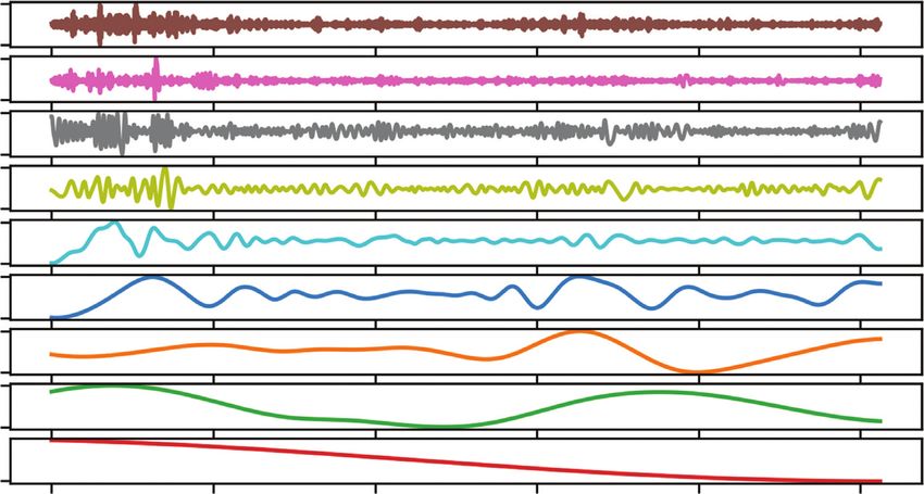
4 Mathematical Problems in Engineering

 LSTM layer LSTM layer

 LSTM unit LSTM unit

 LSTM unit LSTM unit

 Output

 LSTM unit LSTM unit

 Input
 Figure 1: The proposed LSTM model.

the tests are run on Ubuntu 18.04 operation system with 4.3. Experiment I. In this section, the dataset from London
Intel Xeon (R) E5-2650 v4 CPU, GeForce GTX 1080 GPU, Sugar Futures is used to verify the superiority of time series
and 32 GB RAM. Furthermore, to avoid influence of random decomposition technique EMD and the hyperparameters
factor, each method is run 20 times, and the averaging value optimization algorithm TPE, respectively. Three models
is used as final results. such as the model used EMD and TPE combining LSTM
 (TPE-EMD-LSTM), the model used EMD combining LSTM
 (EMD-LSTM), and the single LSTM model are put together
4.1. Data Set Description. The dataset used in this paper was for comparison. In order to have a fair comparison, those
the price of London Sugar Futures from April 2010 to May models are using the same structure which is shown in
2020. Data are fetched from the investing.com. Table 1 Figure 3.
shows the statistic analysis of this dataset. For the LSTM model, we set 100 neurons in each LSTM
 To implement the different experiments, we divide the layer, and with ReLU activation function, the dropout rate is
data into three sets: training set, validation set, and testing 0.5 of dropout layer. The EMD-LSTM model has the same
set. The training set is used to train different models. The hyperparameter with the LSTM model. After optimization,
validation set is used to select the optimal hyperparameters, the obtained optimal hyperparameters of TPE-EMD-LSTM
and the testing set is used to compare the models. The details are summarized in Table 3. Moreover, the RMSE, MAE, and
of those three sets are described in Table 2. MAPE are used to test the performance of the TPE-EMD-
 LSTM and other compared models. The results are shown in
 Table 4. The TPE-EMD-LSTM model attained 2.415 of MAE,
4.2. Performance Evaluation. To assess the superiority of the 0.682 of MAPE, and 2.969 of RMSE. These values are the
proposed hybrid deep learning model, the mean absolute smallest among the three models, indicating the TPE-EMD-
error (MAE), mean absolute percentage error (MAPE), and LSTM model surpasses the LSTM and EMD-LSTM model.
root mean square error (RMSE) are employed for fore- Figure 4 shows the IMFs after decomposition. The perfor-
casting one day ahead sugar price. The formulas of MAE, mance of the EMD-LSTM is better than that of the LSTM in
MAPE, and RMSE are as follows: terms of achieving smaller MAE, MAPE, and RMSE, further
 ascertaining the performance of EMD to handle non-
 m i 
 i�1 yi − y (9) stationarity features in sugar price series.
 MAE � ,
 m
 
 m i /yi
 i�1 yi − y (10) 4.4. Experiment II. In order to further explore the effec-
 MAPE � × 100%,
 m tiveness of TPE-EMD-LSTM, experiment II compares the
 ������������ hybrid deep learning model with two categories of forecasting
 m i�1 yi − y i 2 (11)
 models. For the first category, comparisons are made across
 RMSE � , some basic single models, including the traditional statistical
 m
 model ARIMA, the well-known support vector regression
where m is the number of prediction datasets, yi is the real (SVR) model, and some deep learning models, such as the
 i is the prediction value.
value of feed valve opening, and y DNN model, and the selected single model LSTM, and the

Mathematical Problems in Engineering 5

 Input layer Hidden layer

 Output layer
 Figure 2: The general structure of deep neural networks.

 Table 1: Statistical analysis of sugar price. margin. However, after optimization, the TPE-EMD-DNN
Minimum Maximum Mean Standard deviation Count model performs the best in this section with MAE value of
 2.648, MAPE value of 0.748, and RMSE value of 3.193. It
294.00 876.00 473.95 125.77 2561
 demonstrated the effectiveness of the TPE algorithm.
 Moreover, the TPE-EMD-DNN model shows a significant
 Table 2: Details of the sets. improvement over the EMD-DNN; this not only shows the
Sets Time span Numbers universality of TPE (effective for both LSTM and DNNs) but
Training 19/04/2010–29/05/2018 2063 also shows its effectiveness.
Validation 30/05/2018–22/05/2019 249
Testing 23/05/2019–15/05/2020 249 5. Discussion
 In order to evaluate the performance of the proposed hybrid
proposed hybrid model. The DNN model has the same deep learning model more comprehensively and find
structure of the LSTM model, which is 100 neurons in each methods to improve forecasting capabilities and accuracy,
DNN layer and with ReLU activation function, and the followed by [15, 28, 42, 43], we perform the Die-
dropout rate is 0.5 of dropout layer. For the second category, bold–Mariano (DM) test [44] and improvement percentage.
in order to fully test the hybrid model, two other prediction
models are applied, including TPE-EMD-DNN and EMD-
DNN. After optimization, the obtained optimal hyper- 5.1. DM Test. The DM test is a method for making a
parameters of TPE-EMD-DNN are summarized in Table 5. comparison between the forecasting models and determines
 The performance evaluation metrics for this test are whether forecasts are significantly different. The DM test is
listed in Table 6. The traditional time series model ARIMA described as follows:
has achieved considerable results with MAE value of 4.135, d
MAPE value of 1.189, and RMSE value of 5.747, which DM � ������� Normal(0, 1), (12)
 /T
 2πf
outperform the DNN and EMD-DNN model by a large d

6 Mathematical Problems in Engineering

 Combined dataset

 Input sugar price Training set Testing set
 sequences

 Train forecasting
 Data Use trained models
 models
 preprocessing to forecast future
 Tune Test trained sugar price
 EMD parameters models

 TPE

 Results
 Trained model

 Stage 1: input data & Stage 2: training & testing Stage 2: predicting
 preprocessing forecasting models future sugar price
 Figure 3: Decomposition results of sugar price.

Table 3: Optimal hyperparameters for the TPE-EMD-LSTM EMD-LSTM model will ultimately achieve the most im-
model. portant forecasting.
Hyperparameter Value
l1,n 142 5.2. Improvement Percentage. As discussed in the DM test
l1,a LeakyReLU
 section, the TPE-EMD-LSTM model does significantly
l2,n 150
l2,a LeakyReLU better than all other models. However, the details of fore-
Dropout rate 0.2 casting performance improvement are not clear. Therefore,
Optimizer Rmsprop in this section, we apply three evaluation matrices (IPMAE ,
Batch size 32 IPRMSE , IPMAPE ) to discuss the superiority of TPE and EMD
Learning rate 0.01 more specifically. IPMAE , IPRMSE , and IPMAPE represent the
 improvement percentages of MAE, RMSE, and MAPE,
 respectively. They are defined as follows:
Table 4: Comparison of the predictive accuracy of the various
 MAEm1 − MAEm2
models. IPMAE � × 100%, (13)
Models MAE MAPE RMSE
 MAEm1
LSTM 6.208 1.796 8.187
 RMSEm1 − RMSEm2
EMD-LSTM 4.795 1.352 5.125 IPRMSE � × 100%, (14)
TPE-EMD-LSTM 2.415 0.682 2.969 RMSEm1

 MAPEm1 − MAPEm2
where f is the consistent estimate of spectral density of IPMAPE � × 100%, (15)
 d MAPEm1
loss-differential, d is the mean of the loss-differential be-
tween two forecasts, and T is the length of forecasting time where MAEm1 , RMSEm1 , and MAPEm1 are the MAE, RMSE,
series. The results of the DM test between our proposed TPE- and MAPE values of the compared model and MAEm2 ,
EMD-LSTM and other models are shown in Table 7. RMSEm2 , and MAPEm2 are the MAE, RMSE, and MAPE
 According to Table 7, the DM values range from 4.2 to values of the model being compared. For example, for EMD-
30.4, all far above 2.58, the upper boundary of the 1% DNN vs. DNN, IPMAE shows the improvement percentages
significance level. That is to say, there is a significant dif- of EMD-DNN compared with DNN; if the value of IPMAE is
ference between our proposed TPE-EMD-LSTM model and positive, it means that the EMD-DNN surpasses DNN in
other models. This means that using the proposed TPE- terms of MAE, and vice versa.

Mathematical Problems in Engineering 7

 28.50

 IMF 9 IMF 8 IMF 7 IMF 6 IMF 5 IMF 4 IMF 3 IMF 2 IMF 1
 –28.69
 52.06

 –44.06
 26.19

 –32.66
 58.7

 –53.8
 117.4

 –142.7
 40.26

 –52.26
 73.8

 –92.5
 93.1

 –77.8

 356.3
 0 500 1000 1500 2000 2500

 Figure 4: The process of sugar price forecasting based on the proposed model.

Table 5: Optimal hyperparameters for the TPE-EMD-DNN model. Table 8: Results of improvement percentages.
Hyperparameter Value Compared models IPMAE IPMAPE IPRMSE
l1,n 39 EMD-DNN vs. DNN –11.073 –7.973 7.282
l1,a LeakyReLU EMD-LSTM vs. LSTM 22.761 24.722 37.401
l2,n 186 TPE-EMD-DNN vs. EMD-DNN 81.597 81.149 78.361
l2,a LeakyReLU TPE-EMD-LSTM vs. EMD-LSTM 49.635 49.556 42.068
Dropout rate 0.2
 TPE-EMD-LSTM vs. TPE-EMD-DNN 8.799 8.824 7.015
Optimizer Rmsprop
Batch size 32 ARIMA vs. LSTM 33.392 33.797 29.803
Learning rate 0.01 ARIMA vs. DNN 67.387 67.646 63.889

Table 6: Comparison of the predictive accuracy of the various
 summarizes the improvement percentage results of different
models.
 models.
Models MAE MAPE RMSE
 First of all, compared with DNN, it should be noted that
ARIMA 4.135 1.189 5.747 EMD is more effective for LSTM network. EMD-LSTM vs.
SVR 30.877 9.251 33.884 LSTM shows 22.761, 24.722, and 37.401 of IPMAE , IPMAPE ,
DNN 12.679 3.675 15.915
 and IPRMSE , respectively. However, the EMD-DNN vs. DNN
EMD-DNN 14.083 3.968 14.756
TPE-EMD-DNN 2.648 0.748 3.193 only shows improvement in IPRMSE , and it indicates that the
 DNN is not as good as the LSTM network in capture EMD
 features for time series prediction. For TPE optimization, it
Table 7: DM test results between our proposed model and other shows a huge improvement for EMD-DNN and EMD-
models. LSTM. The TPE optimization enhances the forecasting
Model Value precision to a great extent as the improvement percentages
ARIMA 13.525 relative to the contrasted models are prominent. From the
SVR 7.177 comparison of TPE-EMD-LSTM with TPE-EMD-DNN, it
LSTM 13.039 can be seen that even if TPE optimization brings a huge
EMD-LSTM 30.444 improvement to the DNN, the LSTM network is still better
DNN 13.387
 than the DNN. Finally, ARIMA still outperforms DNN and
EMD-DNN 27.912
TPE-EMD-DNN 4.221
 LSTM, which shows the effectiveness of the traditional time
 series model and can be found in many time series appli-
 cations [30]. However, it also should be noticed that after
 Two comparisons are conducted. Firstly, EMD-DNN hyperparameter optimization, the deep learning-based
and EMD-LSTM are compared with DNN and LSTM, re- model shows significant improvement in forecasting accu-
spectively. Secondly, TPE-EMD-DNN and TPE-EMD- racy and surpassing the ARIMA model.
LSTM are compared with EMD-DNN and EMD-LSTM, In the next step, ensemble forecasting will be investi-
respectively. Moreover, we found that the traditional time gated as it was surged recent years and shows state of the art
series forecasting model ARIMA still has strong perfor- performance on many time series forecasting task [33]. Also,
mance on sugar price forecasting. Therefore, ARIMA is in order to verify its generalizability and robustness, the
compared with LSTM and DNN to discuss the traditional proposed model needs to be applied to predict other food
time series model and deep learning based model. Table 8 commodities.

8 Mathematical Problems in Engineering

6. Conclusions [4] J. E. Meyer and Y. Kim, “An autoregressive forecast of the
 world sugar future option market,” Journal of Financial and
Sugar price forecasting plays a vital role in policy making of Quantitative Analysis, vol. 10, no. 5, pp. 821–835, 1975.
sugar industries. In order to accurately predict sugar price, a [5] Y. Xu, S. Shen, and Z. Chen, “Research on forecast of sugar
hybrid deep learning model that utilizes the merit of time price based on improved neural network,” in Proceedings of
series decomposition technology and a hyperparameter the 2009 Second International Symposium on Intelligent In-
optimization algorithm is proposed. This enhances fore- formation Technology and Security Informatics, pp. 12–15,
 Moscow, Russia, January 2009.
casting performance of the proposed model compared with
 [6] O. Ribeiro and S. M Oliveira, “A hybrid commodity price-
all other models. A large number of experiments have been forecasting model applied to the sugar–alcohol sector,”
conducted to prove the effectiveness of TPE and EMD. Australian Journal of Agricultural and Resource Economics,
Moreover, DM tests are conducted to find improvement vol. 55, no. 2, pp. 180–198, 2011.
percentage and to reveal their specific effects. The DM values [7] N. Silva, I. Siqueira, S. Okida, S. L. Stevan, and H. Siqueira,
from Diebold–Mariano tests between our proposed TPE- “Neural networks for predicting prices of sugarcane deriva-
EMD-LSTM model and other models range from 4.2 to 30.4, tives,” Sugar Tech, vol. 21, no. 3, pp. 514–523, 2019.
all far above 2.58, the upper boundary of the 1% significance [8] M. Pan, C. Li, R. Gao et al., “Photovoltaic power forecasting
level, indicating huge significance between the compared based on a support vector machine with improved ant colony
models. The improvement percentage of the proposed TPE- optimization,” Journal of Cleaner Production, vol. 277, Article
EMD-LSTM model to the other three models (EMD-DNN, ID 123948, 2020.
 [9] Y. LeCun, Y. Bengio, and G. Hinton, “Deep learning,” Nature,
EMD-LSTM, and TPE-EMD-DNN) in the values of
 vol. 521, no. 7553, pp. 436–444, 2015.
IPRMSE is 78, 42, and 7, indicating a significant improve-
 [10] P. Goyal, P. Dollár, R. Girshick et al., Accurate, Large Min-
ment. This enhanced forecasting performance will con- ibatch Sgd: Training Imagenet in 1 Hour, https://arxiv.org/abs/
tribute to the sugar factory’s recruitment plan for new 1706.02677, 2017.
employees and the sugarcane farmers’ plan for planting [11] D. P. Kingma and B. Jimmy, “Adam: a method for stochastic
sugarcane. After finishing this sugar price forecasting work, optimization,” 2014, https://arxiv.org/abs/1412.6980v9.
our future work is to develop ensemble forecasting as it is [12] S. J. Taylor and B. G. Kingsman, “Non-stationarity in sugar
surged recent years and shows state of the art performance prices,” Journal of the Operational Research Society, vol. 29,
on many time series forecasting task [33]. Also, in order to no. 10, pp. 971–980, 1978.
verify its generalizability and robustness, the proposed [13] D. Wang, S. Wei, H. Luo, C. Yue, and O. Grunder, “A novel
model needs to be applied to predict other food hybrid model for air quality index forecasting based on two-
commodities. phase decomposition technique and modified extreme
 learning machine,” Science of The Total Environment, vol. 580,
 pp. 719–733, 2017.
Data Availability [14] S. Zhu, X. Lian, L. Wei et al., “PM2.5 forecasting using SVR
 with PSOGSA algorithm based on CEEMD, GRNN and GCA
The dataset used in this paper was the price of London Sugar considering meteorological factors,” Atmospheric Environ-
Futures from April 2010 to May 2020. Data are fetched from ment, vol. 183, pp. 20–32, 2018.
the investing.com. [15] S. D. Harsh, D. Deb, and M. Josep, “Hybrid machine intel-
 ligent svr variants for wind forecasting and ramp events,”
Conflicts of Interest Renewable and Sustainable Energy Reviews, vol. 108,
 pp. 369–379, 2019.
The authors declare that they have no conflicts of interest. [16] R. Prasad, R. C. Deo, Y. Li, and T. Maraseni, “Input selection
 and performance optimization of ann-based streamflow
 forecasts in the drought-prone murray darling basin region
Acknowledgments using iis and modwt algorithm,” Atmospheric Research,
 vol. 197, pp. 42–63, 2017.
The project was supported by National Natural Science [17] Y. Jiang, G. Huang, X. Peng, Y. Li, and Q. Yang, “A novel wind
Foundation of China (nos. 51465003 and 61763001) and speed prediction method: hybrid of correlation-aided dwt,
Innovation Project of Guangxi Graduate Education (nos. lssvm and garch,” Journal of Wind Engineering and Industrial
YCBZ2020012 and YCBZ2021019). Aerodynamics, vol. 174, pp. 28–38, 2018.
 [18] Z. Hajiabotorabi, A. Kazemi, and F. Faramarz, “Improving
References dwt-rnn model via b-spline wavelet multiresolution to fore-
 cast a high-frequency time series,” Expert Systems with Ap-
 [1] I. Abdul-Aziz and I. Paul Alagidede, “Monetary policy and plications, vol. 138, Article ID 112842, 2019.
 food inflation in South Africa: a quantile regression analysis,” [19] N. K. Yong and N. Awang, “Wavelet-based time series model
 Food Policy, vol. 91, Article ID 101816, 2020. to improve the forecast accuracy of PM10 concentrations in
 [2] R. Trostle, Global Agricultural Supply and Demand: Factors Peninsular Malaysia,” Environmental Monitoring and As-
 Contributing to the Recent Increase in Food Commodity Prices, sessment, vol. 191, no. 2, p. 64, 2019.
 Diane Publishing, Collingdale, PA, USA, 2010. [20] M. Ali and R. Prasad, “Significant wave height forecasting via
 [3] R. Ahmed, V. Sreeram, Y. Mishra, and M. D. Arif, “A review an extreme learning machine model integrated with improved
 and evaluation of the state-of-the-art in pv solar power complete ensemble empirical mode decomposition,” Re-
 forecasting: techniques and optimization,” Renewable and newable and Sustainable Energy Reviews, vol. 104, pp. 281–295,
 Sustainable Energy Reviews, vol. 124, Article ID 109792, 2020. 2019.

Mathematical Problems in Engineering 9

[21] P. Flandrin, G. Rilling, and P. Goncalves, “Empirical mode networks from overfitting,” The Journal of Machine Learning
 decomposition as a filter bank,” IEEE Signal Processing Letters, Research, vol. 15, no. 1, pp. 1929–1958, 2014.
 vol. 11, no. 2, pp. 112–114, 2004. [39] T. Tieleman and G. Hinton, “Lecture 6.5-rmsprop: divide the
[22] Z. Wu, E. Norden, J. M. W. Huang, V. Brian, and X. Chen, gradient by a running average of its recent magnitude,”
 “On the time-varying trend in global-mean surface temper- Coursera: Neural Networks for Machine Learning, vol. 4, no. 2,
 ature,” Climate Dynamics, vol. 37, no. 3, pp. 759–773, 2011. pp. 26–31, 2012.
[23] J. Bedi and D. Toshniwal, “Energy load time-series forecast [40] S. Ruder, An Overview of Gradient Descent Optimization
 using decomposition and autoencoder integrated memory Algorithms, https://arxiv.org/abs/1609.04747v2, 2016.
 network,” Applied Soft Computing, vol. 93, Article ID 106390, [41] T. Nakama, “Theoretical analysis of batch and on-line training
 2020. for gradient descent learning in neural networks,” Neuro-
[24] B. James, R. Bardenet, Y. Bengio, and B. Kégl, “Algorithms for computing, vol. 73, no. 1–3, pp. 151–159, 2009.
 hyper-parameter optimization,” Advances in Neural Infor- [42] G.-F. Fan, S. Qing, H. Wang, W.-C. Hong, and H.-J. Li,
 mation Processing Systems, vol. 24, 2011. “Support vector regression model based on empirical mode
[25] S. Hochreiter and J. Schmidhuber, “Long short-term mem- decomposition and auto regression for electric load fore-
 ory,” Neural Computation, vol. 9, no. 8, pp. 1735–1780, 1997. casting,” Energies, vol. 6, no. 4, pp. 1887–1901, 2013.
[26] Y. Meng, S. Yu, J. Zhang et al., “Hybrid modeling based on [43] R. Karthik and S. Abhishek, Machine Learning Using R: With
 mechanistic and data-driven approaches for cane sugar Time Series and Industry-Based Use Cases in R, Apress, New
 crystallization,” Journal of Food Engineering, vol. 257, York, NY, USA, 2019.
 pp. 44–55, 2019. [44] F. X. Diebold and R. S. Mariano, “Comparing predictive
[27] Y. Meng, J. Zhang, J. Qin et al., “Research on the adaptive accuracy,” Journal of Business & Economic Statistics, vol. 20,
 control in sugar evaporative crystallization using lssvm and no. 1, pp. 134–144, 2002.
 sade-elm,” International Journal of Food Engineering, vol. 15,
 pp. 5-6, 2019.
[28] Y. H. Chen, W.-C. Hong, W. Shen, and N. N. Huang, “Electric
 load forecasting based on a least squares support vector
 machine with fuzzy time series and global harmony search
 algorithm,” Energies, vol. 9, no. 2, 70 pages, 2016.
[29] Y. Meng, S. Yu, Z. Qiu et al., “Modeling and optimization of
 sugarcane juice clarification process,” Journal of Food Engi-
 neering, vol. 291, Article ID 110223, 2021.
[30] B. S. Omer, U. G. Mehmet, and M. O. Ahmet, “Financial time
 series forecasting with deep learning: a systematic literature
 review: 2005–2019,” Applied Soft Computing, vol. 90, Article
 ID 106181, 2020.
[31] C. Baziotis, N. Pelekis, and C. Doulkeridis, “Datastories at
 semeval-2017 task 4: deep lstm with attention for message-
 level and topic-based sentiment analysis,” in Proceedings of the
 11th International Workshop on Semantic Evaluation
 (SemEval-2017), pp. 747–754, Vancouver, Canada, August
 2017.
[32] M. W. Y. Lam, X. Chen, S. Hu et al., “Gaussian process lstm
 recurrent neural network language models for speech rec-
 ognition,” in ICASSP 2019-2019 IEEE International Confer-
 ence on Acoustics, Speech and Signal Processing (ICASSP),
 pp. 7235–7239, Brighton, UK, May 2019.
[33] M. Pawlikowski and A. Chorowska, “Weighted ensemble of
 statistical models,” International Journal of Forecasting,
 vol. 36, no. 1, pp. 93–97, 2020.
[34] K. Swanson, S. Trivedi, J. Lequieu, K. Swanson, and
 R. Kondor, “Deep learning for automated classification and
 characterization of amorphous materials,” Soft Matter, vol. 16,
 no. 2, pp. 435–446, 2020.
[35] J. Lago, F. De Ridder, and B. De Schutter, “Forecasting spot
 electricity prices: deep learning approaches and empirical
 comparison of traditional algorithms,” Applied Energy,
 vol. 221, pp. 386–405, 2018.
[36] I. Goodfellow, Y. Bengio, and A. Courville, Deep Learning,
 MIT Press, Cambridge, MA, USA, 2016.
[37] C. Nwankpa, W. Ijomah, A. Gachagan, and S. Marshall,
 Activation Functions: Comparison of Trends in Practice and
 Research for Deep Learning, https://arxiv.org/abs/1811.
 03378v1, 2018.
[38] N. Srivastava, G. Hinton, A. Krizhevsky, I. Sutskever, and
 R. Salakhutdinov, “Dropout: a simple way to prevent neural