Unit 7 Modeling Two-Variable Data
←
→
Page content transcription
If your browser does not render page correctly, please read the page content below
Unit 7                               Modeling Two-Variable Data

Unit 7: Modeling Two-Variable Data                            1
7.1.1              How can I make predictions?
••••••••••••••••••••••••••••••••••••••••••••••••••••••••••••••••••••••••••••••
Line of Best Fit

7-1.        The championship is on the line between Tinker Toy Tech
            (TTT) and City College. Robbie plans to attend TTT next
            fall and desperately wants to see the game, which has been
            sold out for weeks.

            Surveying the exterior of the stadium, Robbie has
            discovered a small drainage pipe that has a direct view of
            the field. The stadium is being prepared for the big game
            and a maintenance van is currently blocking the view from
            the pipe. The van will be removed just prior to the game so that the view of the field
            will be unobstructed.

            The south end of the field is 50 yards from the end of the pipe and the field runs from
            north to south. The pipe will be at the center of the field when viewed from the south
            end. The width of the field is 53.3 yards (160 feet). Investigate what percentage of
            the field Robbie will be able to see when he looks through the pipe at game time.

            a.    To assist Robbie with this problem we will need to
                  create a model to determine the view based on the
                  distance of the viewed object from the pipe. Your
                  teacher will provide you with a view tube that has the
                  same dimensions as the pipe through which Robbie will
                  be looking. Record the length and diameter of your
                  team’s view tube. Then gather eight data points by
                  measuring two distances: your distance to the wall (in
                  inches) and the width of the field of view (in inches).

                  Length of tube:

                   Distance from wall    Width of field
                   (inches)              of view (inches)

                                                               Problem continues on next page. !
Unit 7: Modeling Two-Variable Data                                                                   2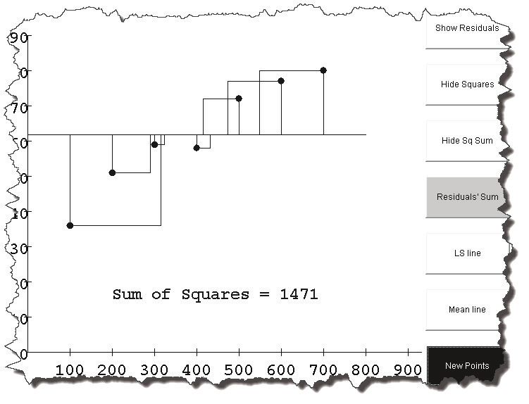
7-1.        Problem continued from previous page.

            b.    Make a scatterplot of your data. Describe the association (the relationship)
                  between the field of view and distance from the wall. When describing an
                  association we always discuss the form (linear, curved, clustered, or gapped),
                  direction (increasing or decreasing), strength (a strong association has very
                  little scatter, while a weak association has a lot of scatter), and outliers (data
                  points that are removed from the pattern the rest of the data makes).

            c.    Draw a line of best fit that models your data and will allow you to make
                  predictions. What is the equation of your line of best fit? In statistics, we write
                  the equation of a line in y = a + bx form.

            d.    Interpret the meaning of the slope in the context of the problem.

7-2.        The closest edge of the field is 50 yards away, and the total length of the playing field
            is 120 yards including the end zones. How many yards does your model predict will
            be visible at the south end of the field? At the north end?

7-3.        Extension: On your paper, sketch the football field and label the dimensions. Using a
            different color, shade the part of the field that Robbie can see.

            a.    Find the area of the field of view.

            b.    What percent of the field will Robbie be able to see?

            c.    The game comes down to the final play in the fourth quarter with TTT driving
                  towards the north end zone. The ends zones are 10yards long. What is the
                  probability Robbie sees the touchdown?

                                        Additional Problems

7-4.        The past and predicted populations for Smallville over a 25-year period are shown
            below.
                         Year         1985 1990 1995 2000 2005 2010
                         Population 248         241     219       216     199      189

            Create a scatterplot and draw the line of best fit for the given data. Use the equation
            of the line of best fit to predict the population of Smallville in 2020.

Unit 7: Modeling Two-Variable Data                                                                     3
7-5.        Sam collected data by sharpening her pencil and comparing the length of the painted
            part of the pencil to its weight. Her data is shown on the graph below:

            a.    Describe the association between weight and length of the pencil. Remember to
                  describe the form, direction, strength, and outliers.

            b.    Make a conjecture about why Sam’s data had an outlier.

            c.    Sam created a line of best fit: < weight > = 1.4 + 0.25 < length > . Describe the
                  slope of her line in context.

            d.    When it was new, Sam’s pencil had 16.75cm of paint. Predict the weight of the
                  new pencil.

            e.    Interpret the meaning of the y-intercept in context.

Unit 7: Modeling Two-Variable Data                                                                    4
7-6. Consumer Reports collected the following data for the fuel efficiency of cars (miles
per gallon) compared to weight (thousands of pounds).
< efficiency > = 49 ! 8.4 < weight >
a. Describe the association between fuel efficiency and weight.
b. Cheetah Motors has come out with a super lightweight roadster that weighs only
1500 pounds. What does the model predict the fuel efficiency will be?
ETHODS AND MEANINGS
Form, Direction, Strength, and Outliers
MATH NOTES
When describing an association between two variables, the form,
direction, strength, and outliers should always be described.
The form (shape) can be linear, curved, clustered, or gapped. The direction
of an association is positive if the slope is positive, and negative or zero
otherwise. The strength is described as strong if there is very little scatter
about the model of best fit, and weak if there is a lot of scatter and the pattern
in the data is not as obvious. Outliers are data points that are far removed
from the rest of the data.
Unit 7: Modeling Two-Variable Data 57.1.2 How close is the model?
••••••••••••••••••••••••••••••••••••••••••••••••••••••••••••••••••••••••••••••
Residuals
7-7. Battle Creek Cereal is trying a variety of packaging for their Toasted Oats cereal.
They wish to predict the net weight of cereal based on the amount of cardboard used
for the package. Below is a list of six current packages.
Packaging Cardboard (in2) Net Weight of Cereal (g)
47 28
69 85
100 283
111 425
125 566
138 850
a. Create a scatterplot. Describe the association between the amount of packaging
and the weight of cereal the package holds in context.
b. Draw a line of best fit that models the data and will allow you to make
predictions. What is the equation of your line? Remember to write the equation
of your line in y = a + bx form.
c. A new experimental “green” package will use 88 square inches of cardboard.
Predict how much cereal this box will hold.
d. A residual is a measure of how far our prediction is from what was actually
observed.
residual = actual – predicted
The 88in2 box will actually hold 198g of cereal. What is the residual for the
88in2 box?
e. Make a point on your scatterplot for the 88in2 box that actually holds 198g of
cereal. We can think about the residual as the distance our actual value is from
the predicted line of best fit. Represent this distance by drawing a vertical
segment from the actual point (88, 198) to the line of best fit.
f. The length of the segment you drew in part (e) represents the residual, that is,
how far our prediction is from what was actually observed. The units are the
same units as the y-axis. How far from the line of best fit (in grams) was the
actual 88in2 box?
g. On your scatterplot, draw the residual segments for all of your other actual
observations.
Unit 7: Modeling Two-Variable Data 67-8. The warehouse store wants to offer a super-sized 250 square inch box.
a. How much cereal do you predict this box will hold?
b. The residual for this box is 2510 grams. What is the actual weight of a 250in2
box?
c. Why do you suppose the residual is so large? Refer to your model and the
scatterplot to make a conjecture about why the predicted weight is so far from
the actual weight.
d. Interpret the meaning of the slope and y-intercept in the context of this problem.
Does the y-intercept make sense in the context of the problem?
7-9. Extension: In a large study by Consumer Reports, the sugar in breakfast cereal was
compared to the calories per serving. Armen was concerned about the percentage of
sugar in his diet, so he created a model that related the sugar in cereal to calories:
= –6.7 + 0.13 .
a. What does a negative residual mean in this context? Is a cereal with a positive
or negative residual better for Armen’s diet?
b. Interpret the meaning of the slope and y-intercept in the context of the problem.
Does the y-intercept make sense in the context of the problem?
Additional Problems
7-10. Ms. Hoang’s class conducted an experiment by rolling a marble down different length
slanted boards and timing how long it took. The results are shown below. Describe
the association.
Unit 7: Modeling Two-Variable Data 77-11. The price of homes (in thousands of dollars) is associated with the number of square
feet in the home. Home prices in Smallville can be modeled with the equation
< priceof home > = 150 + 41 < square feet > . Home prices in Fancyville can be
modeled with the equation < priceof home > = 250 + 198 < square feet > . Ngoc saw
a real estate advertisement for a 4500 square foot home that was selling for $240,000.
Which city should she predict that the home is in?
7-12. A study has been done for a vitamin supplement that claims to shorten the length of
the common cold. The data the scientists collected from ten patients in an early study
are shown in the table below.
Number of months 0.5 2.5 1 2 0.5 1 2 1 1.5 2.5
taking supplement
Number of days 4.5 1.6 3 1.8 5 4.2 2.4 3.6 3.3 1.4
cold lasted
a. Model the data with a line of best fit. According to your model, how many days
do you expect a cold to last for patient taking the supplement for 1.5 months?
b. Calculate the residual for 1.5 months. Interpret the residual in the context of the
problem.
c. Interpret the y-intercept in context.
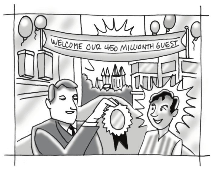
Unit 7: Modeling Two-Variable Data 87-13. WELCOME TO DIZZYLAND!
For over 50 years, Dizzyland has kept track of
how many guests pass through its entrance gates.
Below is a table with the names and dates of
some significant guests.
Name Year Guest
Elsa Marquez 1955 1 millionth guest
Leigh Woolfenden 1957 10 millionth guest
Dr. Glenn C. Franklin 1961 25 millionth guest
Mary Adams 1965 50 millionth guest
Valerie Suldo 1971 100 millionth guest
Gert Schelvis 1981 200 millionth guest
Brook Charles Arthur Burr 1985 250 millionth guest
Claudine Masson 1989 300 millionth guest
Minnie Pepito 1997 400 millionth guest
Mark Ramirez 2001 450 millionth guest
a. If you write the number of guests in millions, this data can be modeled with the
equation < year > = 1958.4 + 0.0995 < number of guests > . If you want to be
Dizzyland’s 1 billionth guest, during what year should you go to the park?
Remember that 1 billion is 1000 millions.
b. What is the residual for Gurt Schelvis?
c. Financial forecasters predicted that Dizzyland would have a positive residual in
2020. Is that good financial news for the park?
d. Interpret the slope and y-intercept in context. Does the y-intercept make sense
in this situation?
Unit 7: Modeling Two-Variable Data 9ETHODS AND MEANINGS
Interpreting Slope and Y-Intercept
MATH NOTES
The slope of a linear association can be described as the amount of
change we expect in the dependent variable when we change the independent
variable by one unit. When describing the slope of a line of best fit, always
acknowledge that you are making a prediction, as opposed to knowing the
truth, by using words like “predict,” “expect,” or “estimate.”
The y-intercept of an association is the same as in algebra. It is the predicted
value of the dependent variable when the independent variable is zero. Be
careful. In statistical scatterplots, the vertical axis is often not drawn at the
origin, so the y-intercept can be someplace other than where the line of best
fit crosses the vertical axis in a scatterplot.
Also be careful of extrapolating the data too far—making predictions that
are far to the right or left of the data. The models we create are often valid
only very close to the data we have collected.
When describing a linear association, you can use the slope, whether it is
positive or negative, and its interpretation in context, to describe the direction
of the association.
Unit 7: Modeling Two-Variable Data 107.1.3 What are the bounds of my predictions?
••••••••••••••••••••••••••••••••••••••••••••••••••••••••••••••••••••••••••••••
Upper and Lower Bounds
7-14. In 1997, an anthropologist discovered an early humanoid
in Europe. As part of the analysis of the specimen, the
anthropologist needed to determine the approximate height
of the individual. The skeletal remains were highly
limited, with only an ulna bone (forearm) being complete.
The bone measured 26.4cm in length. Investigate the
approximate height of the individual that was discovered.
a. In order to approximate the height of the humanoid,
we will need to develop a relationship between the
forearm length and height of a human. We will use
class data to find a representative model. Copy the
chart below and fill in the information for each member of your team. Obtain
data from at least one other team so that you have a minimum of 8 data points.
Name Forearm Length (cm) Height (cm)
b. Using a full sheet of graph paper, plot height vs. forearm length. Since we are
trying to predict height, height is the dependent variable. Start the height axis at
150cm, and the forearm axis at 20cm.
c. Describe the association. Remember to describe form, direction, strength, and
outliers. What may have caused any outliers you might have? Should you
remove them?
d. Graph a line of best fit and find its equation. According to the model that you
created, what would be the height of the humanoid found by the anthropologist?
Unit 7: Modeling Two-Variable Data 117-15. Because the height you found for the humanoid is only a prediction, the actual
observed value may be higher or lower than your prediction. In this problem, you
will find a range of values for your prediction of the humanoid’s height.
a. Look back at your model line.
Identify the point that is farthest
from the line you drew. Find the
residual for this point. In a
different color, draw a dashed line residual
that goes through this maximum
residual point and is parallel to the
line of your model. An example is
shown at right.
b. What is the equation of this line?
You should be able to find the
equation without substituting points.
c. Now draw another dashed line that is on the other side of your model and is the
same distance away as the first dashed line. Find the equation of the second
dashed line.
d. Using the upper and lower bounds of residuals that you just drew, create a range
of values for the height of an individual with a forearm length of 26.4cm.
Additional Problems
7-16. In problem 7-12 you looked at the data for a study conducted on a vitamin
supplement that claims to shorten the length of the common cold. The data is
repeated in the table below:
Number of months 0.5 2.5 1 2 0.5 1 2 1 1.5 2.5
taking supplement
Number of days 4.5 1.6 3 1.8 5 4.2 2.4 3.6 3.3 1.4
cold lasted
a. Create a scatterplot with a line of best fit (or use your scatterplot from
problem 7-12).
b. Draw the upper and lower boundary lines following the process you used on
problem 7-15. What is the equation of the upper boundary line? Of the lower
boundary line?
c. Based on the upper and lower boundary lines of your model, what do you
predict is the length of a cold for a person who has taken the supplement for 3
months?
Problem continues on next page. !
Unit 7: Modeling Two-Variable Data 127-16. Problem continued from previous page.
d. How long do your predict a cold will last for a person who has taken no
supplement? Interpret the y-intercept in context.
e. How long do you predict the cold of a person who has taken 6 months of
supplements will be?
f. If you have a cold, would you prefer a negative or positive residual?
7-17. Fabienne looked at her cell phone bills from the last year, and discovered a linear
relationship between the total cost (in dollars) of her phone bill and the number of
text messages she sent.
a. Do you think that the association is positive or negative? Strong or weak?
b. The upper boundary for Fabienne’s prediction was modeled by
< cost > = 55 + 0.15 < number of texts > . The lower boundary was
< cost > = 25 + 0.15 < number of texts > . What is the equation of Fabienne’s
line of best fit?
c. Interpret the slope of Fabienne’s model in context.
d. Fabienne sent 68 text messages in May. Her residual that month was $9.50.
What was her actual phone bill in May?
ETHODS AND MEANINGS
Residuals
MATH NOTES
We measure how far a prediction made by our model is from the
actual observed value with a residual:
residual = actual – predicted
A residual has the same units as the y-axis. A residual can be graphed with a
vertical segment that extends from the point to the line or curve made by the
best-fit model. The length of this segment (in the units of the y-axis) is the
residual. A positive residual means the predicted value is less than the actual
observed value; a negative residual means the prediction is greater than the
actual.
Unit 7: Modeling Two-Variable Data 137.1.4 How can we agree on a line of best fit?
••••••••••••••••••••••••••••••••••••••••••••••••••••••••••••••••••••••••••••••
Least Squares Regression Line
7-18. The following table shows data for one season of the Chicago Bulls professional
basketball team.
Player Name Minutes Played Total Points in Season
Jordan, Michael 3090 2491
Pippen, Scottie 2825 1496
Harper, Ron 1886 594
Longley, Luc 1641 564
Kerr, Steve 1919 688
Rodman, Dennis 2088 351
Wennington, Bill 1065 376
Haley, Jack 7 5
Buechler, Jon 740 278
Simpkins, Dickie 685 216
Edwards, James 274 98
Caffey, Jason 545 182
Brown, Randy 671 185
Salley, John 191 36
checksum 17627 checksum 7560
a. Chicago Bulls team member Toni Kukoc was inadvertently left off of the list.
We would like to predict how many points he made in the season. Before you
learned about lines of best fit, your best prediction would have been to predict
that he scored the average amount. Predict the number of points Toni Kukoc
scored by finding the mean number of points team members scored.
b. Regardless of whether Toni Kukoc actually played only a few minutes or a large
number of minutes, our best prediction is that he made 540 points. Our
prediction equation is y = 540 . Obtain a Lesson 7.1.4 Resource Page from your
teacher. Sketch a vertical segment to the line y = 540 for each of the residuals.
Calculate the residuals from the expected y = 540 for each of the players.
c. Find the sum of the residuals for the prediction model y = 540 . Explain why
your sum of the residuals makes sense.
d. Who is an outlier for this data? What is his residual?
e. Is a negative or positive residual better for a player’s reputation?
Unit 7: Modeling Two-Variable Data 147-19. Of course, a line of best fit will make better predictions than simply predicting
“average” for each player. Now we will investigate lines of best fit.
a. Sum the absolute values of the residuals for the model y = 540 . Why do you
think are we interested in the absolute values of the residuals?
b. Using a different color, sketch a line of best fit for the scatterplot on the
resource page. Write the equation for your model that predicts the number of
points a player will score.
c. Calculate the sum of the absolute values of the residuals for your line of best fit.
Explain why your sum of the absolute values of the residuals is much less than
when you used the model y = 540 .
d. Since residuals measure how far the prediction is away from the actual observed
data, the ideal model will minimize the residuals. Did any of your classmates
have a model that had a smaller sum of residuals than yours?
e. Sometimes there are several different lines of best fit that can be drawn with the
same sum of the absolute values of the residuals. To assure that we have a
unique line of best fit, mathematicians often use the sum of the squares of the
residuals instead. What is the sum of the squares of the residuals for the model
y = 540 ? For your line of best fit? Did any classmate have a better model than
yours because they had a smaller sum of the squares of the residuals?
7-20. The least squares regression line (LSRL) is the line that has the smallest possible
value for the sum of the squares of the residuals.
a. Use your calculator to make a scatterplot and find the LSRL. Sketch your graph
and LSRL on your paper. A sketch is a quick general drawing of what you see
on your calculator screen. It is usually not drawn on graph paper and therefore
points are not plotted perfectly. But a sketch always has a scale on the x- and
y-axes! Often, key points are labeled with their coordinates, and lines are
labeled with their equation.
b. Find the residuals for the LSRL on your calculator. What is the sum of the
squares of the residuals of the LSRL the calculator found? Was it less than your
sum of squares?
c. Toni Kukoc played for 1065 minutes. How many points does the LSRL predict
for Toni Kukoc?
d. Interpret the slope and y-intercept of the model in context. Explain why this
LSRL model is not reasonable for players that played less than about 350
minutes.
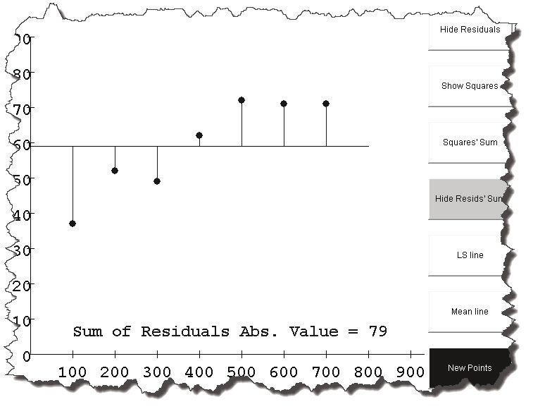
Unit 7: Modeling Two-Variable Data 157-21. Extension: Investigate the LSRL and minimizing the squares of the residuals using a
computer.
a. With your Internet browser, go to
http://hadm.sph.sc.edu/Courses/J716/demos/LeastSquares/LeastSquaresDemo.html
b. Using the rectangle “buttons” on the right side of the screen, show the residuals
and residuals sum, but hide the squares, and the squares sum. Press the mean
line button. Your screen should look something like this:
c. Drag the mean line to reduce the sum of residuals. What is the lowest sum of
residuals you can get?
d. Since there is sometimes more than one line that has the least sum of residuals,
mathematicians minimize the sum of the squares of the residuals instead. Using
the rectangle “buttons” on the right, show the squares and the squares sum, but
hide the residuals, and the residuals sum. Press the mean line button. Your
screen should look something like this:
e. Drag the mean line to make the squares as small as possible and reduce the sum
of squares residuals. What is the lowest sum of squares you can get?
f. Press the LS line button to find the LSRL line. There is only one LSRL line
that minimizes the sum of the squares. All other lines have a larger sum of
squares.
Unit 7: Modeling Two-Variable Data 16Additional Problems
7-22. Robbie’s class collected the following view tube data in problem 7-1.
Distance from wall (inches) Width of field of view (inches)
144 20.7
132 19.6
120 17.3
108 16.2
96 14.8
84 13.1
72 11.4
60 9.3
checksum 816 checksum 122.4
a. Use your calculator to make a scatterplot and graph the least squares regression
line (LSRL). Sketch the graph and LSRL on your paper. Remember to put a
scale on the x-axis and y-axis of your sketch. Write the equation of the LSRL
rounded to four decimal places.
b. With your calculator, find the residuals like you did in part (b) of problem 7-20.
Make a table with the distance from wall (inches) as the first column, and
residuals (inches) in the second column. What is the sum of the squares of the
residuals?
7-23. Students in Ms. Zaleski’s class cut circular disks from cardboard. The weight and
radius were recorded. The information is shown in the table below. Consider the
radius the independent axis.
radius (cm) 9.6 9 7.7 6.3 5.3 4.7 3.7 2.4 1.3
weight (g) 5.4 4.6 3.4 2.3 1.6 1.2 0.8 0.3 0.1
a. Make a scatterplot for the data on your calculator and sketch it on to your paper.
Describe the association between weight and radius.
b. What is the equation of the LSRL you could use to model this data? Sketch the
LSRL on your paper.
c. Does it seem appropriate to model this data with a line?
Unit 7: Modeling Two-Variable Data 17ETHODS AND MEANINGS
Least Squares Regression Line
MATH NOTES
There are two reasons for modeling scattered data with a best-fit line.
One is so that the trend in the data can easily be described to others without
giving them a list of all the data coordinates. The other is so that predictions
can be made about points for which we do not have actual data.
A consistent best-fit line for data can be found by determining the line
that makes the residuals, and hence the square of the residuals, as small as
possible. We call this line the least squares regression line and abbreviate
it LSRL. Our calculator can find the LSRL quickly. Statisticians prefer the
LSRL to other best-fit lines because there is one unique LSRL for any set of
data. All statisticians, therefore, come up with exactly the same best-fit line
and can make similar descriptions of, and predictions from, the scattered
data.
Unit 7: Modeling Two-Variable Data 187.2.1 When is my model appropriate?
••••••••••••••••••••••••••••••••••••••••••••••••••••••••••••••••••••••••••••••
Residual Plots
7-24. Previously, you may have completed an observational study using tubular vision.
Typical data is shown in the table below.
Distance from wall (inches) Width of field of view (inches)
144 20.7
132 19.6
120 17.3
108 16.2
96 14.8
84 13.1
72 11.4
60 9.3
checksum 816 checksum 122.4
a. Create a scatterplot and LSRL on your calculator and sketch them. What is the
equation of the LSRL?
b. When entering the data in her calculator, Amy accidentally entered (144, 10.7)
for the first data point. Make this change to your data and sketch the new point
and new LSRL in a different color. Will Amy’s predictions for the field of view
be too large or too small?
7-25. Giulia’s father would like to open a restaurant, and is deciding how much to charge
for the toppings on pizza. He sends Giulia to eight different Italian restaurants around
town to find out how much they each charge. Giulia comes back with the following
information:
# toppings on pizza cost ($)
(not including cheese)
Paolo’s Pizza 1 10.50
Vittore’s Italian 3 9.00
Ristorante Isabella 4 14.00
Bianca’s Place 6 15.00
JohnBoy’s Pizza Delivery 3 12.50
Ristorante Raffaello 5 16.50
Rosa’s Restaurant 0 8.00
House of Pizza Pie 2 9.00
Problem continues on next page. !
Unit 7: Modeling Two-Variable Data 197-25. Problem continued from previous page.
a. Sketch the scatterplot, and add a model of the data with an LSRL equation.
Describe the form, direction, and strength of the association.
b. Predict what Giulia’s father should charge for a two-topping pizza.
c. Mark the residuals on the scatterplot. If you want to purchase an inexpensive
pizza, should you go to a store with a positive or negative residual?
d. What is the sum of the residuals? Are you surprised at this result?
e. Make a residual plot with your calculator, with the x-axis representing the
number of pizza toppings, and the y-axis representing the residuals. The
random scatter of the points on the residual plot (there does not appear to be any
kind of shape or pattern to the plotted points) means the model fits through the
data points well. That is, our LSRL linear model is appropriate.
7-26. Dry ice (frozen carbon dioxide) evaporates at room temperature. Giulia’s father uses
dry ice to keep the glasses in the restaurant very cold. Since dry ice evaporates in the
restaurant cooler, Giulia was curious how long a piece of dry ice would last. She
collected the following data:
# of hours after noon Weight of dry ice (g)
0 15.3
1 14.7
2 14.3
3 13.6
4 13.1
5 12.5
6 11.9
7 11.5
8 11.0
9 10.6
10 10.2
a. Sketch the scatterplot and LSRL of this data.
b. Sketch the residual plot to determine if a linear model is appropriate. Make a
conjecture about what the residual plot tells you about the shape of the original
data Giulia collected.
Unit 7: Modeling Two-Variable Data 207-27. A study by one states Agricultural Commission plotted the number of avocado farms
in each county against that county’s population (in thousands). The LSRL is
= 9.37 + 3.96 . The residual plot
follows.
a. Do you think a linear model is appropriate? Why or why not?
b. What is the predicted number of avocado farms for a county with a population
of 62,900 people?
c. Estimate the actual number of avocado farms in a county with 62,900 residents.
7-28. Sophie and Lindsey were discussing what it meant for a residual plot to have random
scatter. Sophie said the points had to be evenly scattered over the whole plot.
Lindsey heard her Dad say that stars in the night sky can be considered to be
randomly distributed even though the stars sometimes appear in clusters and
sometimes there are large expanses of nothing in the sky.
a. Help Sophie and Lindsey see what a random plot looks like. Generate 25
random numbers and store them in List1 by entering , PRB, rand(25),
¿, y, d on your calculator. Then generate 25 additional random
numbers and store them in List2 by entering , PRB, rand(25), ¿,
y, we. Consider the random numbers in List1 the x-coordinate, and the
numbers in List2 the y-coordinate. Make a scatterplot of the 25 random points.
Press q ® as a shortcut to set the window correctly. Share your random
plot with your teammates.
b. Make another scatterplot like you did in part (a). What do you notice about
random scatter?
Unit 7: Modeling Two-Variable Data 217-29. Extension: For which of the residual plots below is a linear model appropriate?
Plot A Plot B Plot C
7-30. Extension: Predict what a sketch of the scatterplot and the LSRL might look like for
each of the residual plots above.
Additional Problems
7-31. Sam collected data in problem 7-5 by sharpening her pencil and comparing the length
of the painted part of the pencil to its weight. Her data is listed in the table below.
Length of paint (cm) 13.7 12.6 10.7 9.8 9.3 8.5 7.2 6.3 5.2 4.5 3.8
Weight (g) 4.7 4.3 4.1 3.8 3.6 3.4 3.0 2.8 2.7 2.3 2.3
a. Graph the data on your calculator and sketch the graph on your paper.
b. What is the equation of the LSRL? Sketch it on your scatterplot.
c. Create a residual plot and sketch it on your paper.
d. Interpret your residual plot. Does it seem appropriate to use a linear model to
make predictions about the weight of a pencil?
e. Sam’s pencil, when it was new, had 16.75cm of paint and weighed 6g. What
was the residual? What does a positive residual mean in this context?
Unit 7: Modeling Two-Variable Data 227-32. Paul and Howard made a conjecture that the average size of TV screens has increased
rapidly in the last decade—they both remember the relatively small TVs they had
when they were in elementary school. They collected data about the size of TVs each
year for several years (www.flowingdata.com).
Year 2002 2003 2004 2005 2006 2007 2008 2009
Average size of TV (in) 34 34 46 42 42 46 46 46
a. Make a scatterplot of size over time. Enter the year 2002 as year “2.”
b. What is the equation of the LSRL? Sketch it.
c. Use a residual plot to analyze whether a linear plot is appropriate.
d. Describe the association between average size of TVs and time. Your
description should include an interpretation of the slope.
e. Predict the average size of a TV screen in 2015. How confident are you that
your prediction will be correct?
f. Interpret the y-intercept in context. Does it make sense?
g. The largest residual is 6.57. What does this mean in context?
h. What are the equations of the upper and lower bounds? Graph them on your
scatterplot with dashed lines.
7-33. The winning times in various swim meets at Smallville High School were compared
to the year. The residual plot follows:
a. Sketch what the original scatterplot may have looked like.
b. What does the residual plot tell you about predictions made with the LSRL in
more recent years?
Unit 7: Modeling Two-Variable Data 23ETHODS AND MEANINGS
Residual Plots
MATH NOTES
A residual plot is created in order to analyze the appropriateness of a
best-fit model. A residual plot has an x-axis that is the same as the
independent variable for the data. The y-axis of a residual plot is the residual
for each point. Recall that residuals have the same units as the dependent
variable of the data.
If a linear model fits the data well, no interesting pattern will be made by the
residuals. That is because a line that fits the data well just goes through the
“middle” of all the data.
A residual plot can be used as evidence that the description of the form of a
linear association has been made appropriately.
Unit 7: Modeling Two-Variable Data 247.2.2 How can I measure my linear fit?
••••••••••••••••••••••••••••••••••••••••••••••••••••••••••••••••••••••••••••••
Correlation
You may recall that to find the equation of the LSRL, your calculator minimized the sum of the
squares of the residuals. The smaller the sum of the squares, the closer the data was to the line of
best fit. However, the magnitude of the sum of squares depends on the units of the variables
being plotted. Therefore the sum of squares cannot be compared between scatterplots with
different units.
The correlation coefficient, r, is a measure of how much or how little data is scattered around the
LSRL. That is, if you have already plotted the residuals and decided that the linear model is a
good fit, the correlation coefficient, r, is a measure of the strength of a linear association.
The correlation coefficient does not have units, so it is useful no matter what the units of the
variables are.
7-34. This problem will lead you through an investigation of r to determine its properties.
a. Choose any two points that have integer coordinates and a positive slope
between them. Write the coordinates of these original points down—you will
need them later. Each member in your team should choose different points.
b. Enter the coordinates of your two points (not your teammates’ points!) into
List1 and List2 of your calculator. Find the LSRL between your two points and
record the value of r. The LSRL model is a perfect fit with your data. Discuss
your results with your team. (When you calculate the LSRL, your calculator
reports the correlation coefficient on the same screen as it reports the slope and
y-intercept. If your TI calculator does not calculate r, press y, N,
DiagnosticOn, Í, Í and try again.)
c. Each member of your team should choose two new points that have a negative
slope between them. Remove the old data from your lists, and enter the two
new points. Record the value of r. Again, the LSRL model is a perfect fit with
your data. Discuss this with your team.
d. What happens when you have more than two data points? Clear your lists and
re-enter your original points from part (a). Find a third point that results in
r = 1 . How can you describe the location of all possible points that result in
r = 1?
Unit 7: Modeling Two-Variable Data 257-35. What happens when the model is a poor fit?
a. Clear your lists and enter the original points from part (a). Enter a third point
that is not on the line. Graph the scatterplot and LSRL. What happens to the
value of r? (Hint: To make quick scatterplots without setting the window each
time, press y , to set up a scatterplot, and then press q ® to get
a quick scatterplot of your three points.)
b. Delete the third point from your list. If you have not already, can you enter a
third point which makes the slope of the LSRL negative? What happens to r?
c. Choose and check points until you find a third point which makes r close to zero
(say, between –0.2 and 0.2).
7-36. Discuss with your team and record all of your conclusions from this investigation.
7-37. The following scatterplots have correlation r = !0.9, r = !0.6, r = 0.1, and r = 0.6.
Which scatterplot has which correlation coefficient, r?
a. b.
c. d.
Unit 7: Modeling Two-Variable Data 267-38. Previously you may have conducted an observational study using tubular vision.
Typical data is shown in the table below. The LSRL is y = 1.66 + 0.13x .
Distance from wall (in) Field of view (in)
144 20.7
132 19.6
120 17.3
108 16.2
96 14.8
84 13.1
72 11.4
60 9.3
checksum 816 checksum 122.4
a. Is the association in the tubular vision study strong or weak? Find the
correlation coefficient.
b. Describe the form, direction, strength, and outliers of the association.
c. You already know a graphical way to determine if the “form” is linear. A
mathematical description of “direction” is the slope. A mathematical
description of “strength” is the correlation coefficient. Describe the form,
direction, and strength in more mathematical terms than you did in part (b).
7-39. Extension: A computer will help us explore the correlation coefficient further.
a. Go to http://illuminations.nctm.org/LessonDetail.aspx?ID=L456#qs .
b. Add some points to the graph by clicking on the graph. Press “Show Line” to
plot the LSRL line and calculate the correlation coefficient, r. Press Ctrl-click
to delete a point. Hold Shift-click to drag a point. Your screen should look
something like this:
Problem continues on next page. !
Unit 7: Modeling Two-Variable Data 277-39. Problem continued from previous page.
c. Create the following scatterplots and record r:
• Strong positive linear association
• Weak positive linear association
• Strong negative linear association
• No linear association (random scatter)
d. Use just five points to make a strong negative linear association (say r < !0.95 ).
Drag one of the points around to observe the effect on the slope and correlation
coefficient. Can you make the slope positive by dragging just one point?
Additional Problems
7-40. The average wage for a technical worker over a 10-year period is shown below.
Year 1 2 3 4 5 6 7 8 9 10
Wage ($) 12.00 13.25 14.00 16.00 17.00 18.00 19.50 21.00 22.00 23.25
a. Sketch a scatterplot showing the association between the average wage and the
year.
b. Sketch the residual plot. Is a linear model appropriate?
c. What is the correlation coefficient? What does it tell you?
7-41. Paul and Howard collected data about the size of TVs for almost a decade.
Year 2002 2003 2004 2005 2006 2007 2008 2009
Average size of TV (in) 34 34 46 42 42 46 46 46
(www.flowingdata.com)
a. Make the scatterplot on your calculator without drawing the LSRL. Enter year
2002 as “2.” Make a conjecture about what the correlation coefficient, r, will
equal. Will it be positive or negative?
b. Check your answer to part (a) by finding the correlation coefficient.
Unit 7: Modeling Two-Variable Data 287-42. Fire hoses come in different diameters. How far
the hose can throw water depends on the
diameter of the hose. The Smallville Fire
Department collected data on their fire hoses.
Their residual plot is shown at right.
a. Sketch what the original scatterplot must
have looked like.
b. What does the residual plot tell you about
the LSRL model the fire department used?
c. Find the worst prediction made with the LSRL.
How different was the worst prediction from
what was actually observed? Explain in
context.
7-43. Scientists hypothesized that dietary fiber would impact the blood cholesterol level of
college students. They collected data and found r = –0.45 with a scattered residual
plot. Interpret the scientists’ findings in context.
7-44. Make a conjecture about what r is for the following scatterplot. Make a conjecture of
where the LSRL might fall.
Unit 7: Modeling Two-Variable Data 297.2.3 What does the correlation mean?
••••••••••••••••••••••••••••••••••••••••••••••••••••••••••••••••••••••••••••••
Interpreting Correlation in Context
Although the correlation coefficient is widely used to describe the amount of scatter in a linear
association, unfortunately it does not have a real-world contextual meaning. In Lesson 7.1.3 you
studied the association between the height of a human and his/her forearm length. If you had
calculated that r = 0.8 you would know that the association was moderately strong and positive,
but you would not know much else about the strength of the association.
Fortunately the value of r 2 does have a contextual real-world meaning. If in the humanoid
problem r = 0.8 , then r 2 = 0.64 . By tradition, we write R 2 and express it as a percent. R 2
does not have a name, so we say, “R-squared is 64%.” Then we can say that 64% of the
variability in human height can be explained by a linear relationship with forearm size.
7-45. In Lesson 7.1.3, Kerin discovered that a human’s height is associated with their
forearm length. Kerin is curious whether or not the same thing is true for foot size.
a. It wasn’t practical for Kerin to measure her classmates’ feet, so Kerin collected
the following shoe-size data from her classmates. For Kerin’s data below,
r = 0.86 . Using R 2 in a sentence, what can you say about the variation in
height in Kerin’s class?
shoe size height (cm) shoe size height (cm)
6 153 9 167
8 160 7.5 162
7 158 8 162
8.5 161 7.5 166
8 168 8.5 167
8 166 6.5 159
8.4 164 7 160
6.5 156 9 169
10 170 8 164
9.5 167 8.5 166
7.5 158 7.5 159
7 158 9.5 169
8 161 checksum 198.9 checksum 4070
b. If only a portion of the variation in height can be explained by shoe size, what
other factors might go into determining someone’s height?
Unit 7: Modeling Two-Variable Data 307-46. Suppose Alyse collected the following unusual data for students in her class:
shoe size height (cm)
6 154
7! 160
8 162
8! 164
10 170
a. What is the correlation coefficient? In the context of this problem, what does
the correlation coefficient tell Alyse about the variation in heights?
b. What can Alyse say about the predicting height in her class?
7-47. Holly created the following scatterplot for the girls in her class.
a. What do you notice about this data? What do you suppose the correlation
coefficient is? Write a sentence about the variability in girls’ height in Holly’s
class.
b. The best prediction Holly can make is to predict a girl has average height no
matter what her shoe size is. According to the U.S. Centers for Disease Control
National Health Statistics Report, the average height of women in the U.S. is
162.2cm. What would the line of best fit look like? What is the equation of the
line of best fit?
Unit 7: Modeling Two-Variable Data 317-48. When Giulia went around town comparing the cost of toppings at pizza parlors, she
gathered this data.
# toppings on pizza cost ($)
(not including cheese)
Paolo’s Pizza 1 10.50
Vittore’s Italian 3 9.00
Ristorante Isabella 4 14.00
Bianca’s Place 6 15.00
JohnBoy’s Pizza Delivery 3 12.50
Ristorante Raffaello 5 16.50
Rosa’s Restaurant 0 8.00
House of Pizza Pie 2 9.00
a. What is the LSRL? Interpret the y-intercept in context.
b. What are the correlation coefficient and R 2 ?
c. Describe the association. Use slope when describing the “direction,” and use a
sentence about R 2 when describing strength.
7-49. Giulia’s father finally opened his pizza parlor. He charges $7.00 for each cheese
pizza plus $1.50 for each additional topping.
a. Choose four or five points and make a scatterplot of the cost of pizza versus the
number of toppings at Giulia’s father’s pizza parlor. What is the LSRL?
Interpret the slope and y-intercept in context.
b. What is r ? R 2 ? Write a sentence about the variation in cost of pizza at this
parlor.
7-50. A researcher wanted to see the effect of the number of hours spent watching TV had
on students’ grade point averages. He found r = !0.72 . Interpret the researcher’s
results.
7-51. Extension: Suppose you found that the correlation between the life expectancy of
citizens in a nation and the average number of TVs in households in that nation is
r = 0.89 . Does that mean that watching TV helps you live longer?
Unit 7: Modeling Two-Variable Data 32Additional Problems
7-52. Consumer Reports collected the following data for the fuel efficiency of cars (miles
per gallon) compared to weight (thousands of pounds).
< efficiency > = 49 ! 8.4 < weight >
r = –0.903
a. Interpret R-squared in context.
b. Interpret the slope in context.
7-53. Data for a study of a vitamin supplement that claims to shorten the length of the
common cold is shown below:
Number of months 0.5 2.5 1 2 0.5 1 2 1 1.5 2.5
taking supplement
Number of days 4.5 1.6 3 1.8 5 4.2 2.4 3.6 3.3 1.4
cold lasted
a. You previously created a linear model for this data by “eyeballing” it. Now
create a model that is consistent with your classmates by finding the LSRL.
Sketch the graph and the LSRL.
b. Is a linear model appropriate? Provide evidence.
c. Find r and R-squared. Interpret R-squared in context.
d. Describe the association. Make sure you describe the form and provide
evidence for the form. Provide numerical values for direction and strength and
interpret them in context. Describe any outliers.
Unit 7: Modeling Two-Variable Data 337-54. Scientists were concerned that there might be arsenic in unregulated drinking wells
and that people were ingesting arsenic, a poison, by drinking from these wells.
Arsenic in the human body, like many toxins, can most easily be measured in
toenails. How much has collected in the toenails is an indication of how much
arsenic is in the whole body. In a study in the journal Cancer Epidemiology,
Biomarkers and Prevention, the arsenic level in 21 people was measured along with
the unregulated drinking wells from which each of them obtained their water.
arsenic in water arsenic in toenail arsenic in water arsenic in toenail
(ppb) (ppm) (ppb) (ppm)
0.87 0.119 46.0 0.832
0.21 0.118 19.4 0.517
0 0.099 137 2.252
1.15 0.118 21.4 0.851
0 0.277 17.5 0.269
0 0.358 76.4 0.433
0.13 0.080 0 0.141
0.69 0.158 16.5 0.275
0.39 0.310 0.12 0.135
0 0.105 4.10 0.175
0 0.073 checksum 341.86 checksum 7.695
Fully describe all aspects of the association in context. Include appropriate graphs.
Unit 7: Modeling Two-Variable Data 34ETHODS AND MEANINGS
MATH NOTES Correlation Coefficient
The correlation coefficient, r, is a measure of how much or how little
data is scattered around the LSRL; it is a measure of the strength of a linear
association. The correlation coefficient can take on values between –1 and 1.
If r = 1 or r = !1 the association is perfectly linear. There is no scatter
about the LSRL at all. A positive correlation coefficient means the trend is
increasing (slope is positive), while a negative correlation means the
opposite. A correlation coefficient of zero means the slope of the LSRL is
horizontal and there is no linear association whatsoever between the
variables.
The correlation coefficient does not have units, so it is a useful way to
compare scatter from situation to situation no matter what the units of the
variables are. The correlation coefficient does not have a physical meaning
other than as an arbitrary measure of strength.
The value of the correlation coefficient squared, however, does have a
contextual real-world meaning. R-squared, the correlation coefficient
squared, is written as R 2 and expressed as a percent. Its meaning is that R 2 %
of the variability in the dependent variable can be explained by a linear
relationship with independent variable. The rest of the variability is explained
by other differences in the factors being measured.
The correlation coefficient, along with the interpretation of R 2 , is used to
describe the strength of a linear association.
Unit 7: Modeling Two-Variable Data 357.2.4 What if a line does not fit the data?
••••••••••••••••••••••••••••••••••••••••••••••••••••••••••••••••••••••••••••••
Curved Regression Models
So far we have looked at a variety of linear models, but what happens when the best model is not
linear?
7-55. Top-It-Off Incorporated makes numerous lids for a
variety of containers. Some of the most popular
covers they produce are circular lids for oil drums
and other cylindrical containers. Although the lids
are ordered by the diameter of the circle, the price is
set by the amount of metal used. Top-It-Off needs
to set up a price structure that relates the weight of a
lid to its diameter. Below is a list of current prices
for the standard size lids currently produced.
Diameter of lid (in) Weight of metal (lbs)
10 3.9
12 5.7
16 10.1
20 15.7
24 22.6
30 35.3
36 50.9
40 62.8
a. The company analyst needs to find a good model for the weight as a function of
the diameter. Use your calculator to create a scatterplot of your data and sketch
the results.
b. The data appears to have only a slight curve. Based on the scatterplot alone,
you may think a linear model would be a good fit. Use your calculator to find
the equation of the LSRL. Add this line to the sketch from part (a).
c. Make a residual plot of the regression. What conclusion can you draw about
your linear model?
d. What is the correlation coefficient? Write a sentence about R-squared in
context.
Unit 7: Modeling Two-Variable Data 367-56. A BETTER MODEL
a. Thinking about the relationship between the weight and the area, why is it
reasonable to assume that a quadratic equation will model this relationship
better?
b. Use your calculator to find the quadratic regression equation. Add this graph to
the scatterplot sketch. Be sure to write the equation near the graph.
c. Based on the calculator display, which model is a better fit for the data?
d. Make a residual plot of the quadratic regression. Compare the residual plot of
the linear regression to the residual plot of the quadratic regression. Which
model is a better fit for the data?
You may be tempted to compare the R 2 your calculator reports for the
quadratic regression with the R 2 from your linear model in the previous
problem. Although both values are called R 2 , unfortunately they are calculated
differently and cannot be compared.
7-57. Recall that Giulia’s father uses dry ice to keep the glasses in his restaurant very cold.
The dry ice evaporates in the restaurant cooler as follows:
# hours after noon Weight of dry ice (g)
0 15.3
1 14.7
2 14.3
3 13.6
4 13.1
5 12.5
6 11.9
7 11.5
8 11.0
9 10.6
10 10.2
a. Recreate the scatterplot of this data on your calculator. Sketch the plot. What
does the residual plot tell you about the original data Giulia collected.
b. Using your knowledge from Algebra 2, what kind of parent function might fit
this data better?
c. Now use your calculator to find the exponential regression equation. Add this
graph to the scatterplot sketch. Be sure to write the equation near the graph.
Problem continues on next page. !
Unit 7: Modeling Two-Variable Data 377-57. Problem continued from previous page.
d. Based on the scatterplot alone, does the linear model or the exponential model
fit the data better?
e. Make a residual plot of the exponential regression. Comment on the
appropriateness of the exponential model.
7-58. Extension: In the early 1970’s, there was speculation of a
tenth planet in our solar system beyond Pluto. This planet
was given the name Planet X. (At that time, Pluto was
believed to be a planet.) Feeling nostalgic for the
seventies, Disco Dan has decided to do a study on this
mysterious planet. The first part of the study is to
determine the length of one Planet X year. Dan gathers the
following set of data that shows the planets, their distances
from the sun, and the length of their year (measured in
number of Earth years).
Distance from sun Length of year
Planet
(millions of miles) (Earth years)
Mercury 36.0 0.241
Venus 67.0 0.615
Earth 93.0 1.000
Mars 141.5 1.880
Jupiter 483.0 11.900
Saturn 886.0 29.500
Uranus 1782.0 84.000
Neptune 2793.0 165.000
Pluto 3670.0 248.000
checksum 9951.5 checksum 542.136
a. Use your calculator to create a scatterplot of the data above. Sketch the graph
on your paper.
b. Find an LSRL for the data. Is it a good fit?
c. Although a line seems to fit fairly well, we cannot be confident it is the best fit.
Since the graph curves, see if an exponential model would make a better fit.
d. How well does a quadratic model fit? Which model (linear, exponential, or
quadratic) made the best predictions?
7-59. Extension: Use the best model from part (d) in problem 7-58 above to predict the
length of the celestial year on Mercury and on Venus. What problem do you notice
with the quadratic model?
Unit 7: Modeling Two-Variable Data 387-60. Extension: Disco Dan really wants an accurate model for
his planet of the 1970’s, and the quadratic model gives an
illogical prediction for Mercury and Venus.
a. After learning from a physicist that the length of a
celestial year varies with a power of the distance, Dan
decides to try a power function. How well does a
power regression fit your data? What is the equation?
b. According to the legend, Planet X is 5180 million
miles away from the sun. How long is one of its years
compared to a year on Earth?
Additional Problems
7-61. Eeeeew! Hannah left an egg salad sandwich sitting in
her locker over the weekend, and when she got back
on Monday it had started to get moldy. “Perfect!”
said Hannah. “I can use this for my biology project.
I’ll study how quickly mold grows. My hypothesis
will be that it grows faster and faster.”
Hannah knew that first she had to gather data. Using
a transparent grid, she estimated that about 12% of
the surface of the sandwich had mold on it. She put it
back in her locker, and on Tuesday she estimated that
15% was moldy. But then she forgot about it until Friday, when it was about 29%
was moldy. Now what? How could she get the missing days’ data without wasting
another sandwich?
“I know,” said Hannah. “I’ll use the regressions I’ve learned to model the data with
an equation that will get me reasonable predictions of the missing data.”
a. Create a scatterplot and sketch it. Is a linear model reasonable?
b. Based on the story, what kind of equation do you think will best fit the
situation?
c. Fit the data with an exponential model and write the equation. Fill in Hannah’s
missing data by making predictions of what percentage of sandwich was
covered on Wednesday and Thursday.
Unit 7: Modeling Two-Variable Data 397-62. In problem 7-7, Battle Creek Cereal was trying a variety of packaging for Toasted
Oats cereal. They wish to predict the net weight of cereal based on the amount of
cardboard used for the package. Below is a list of six current packages.
Packaging cardboard (in2) Net weight of cereal (g)
47 28
69 85
88 198
100 283
111 425
125 566
138 850
checksum 678 checksum 2435
a. In a previous lesson, you may have hand-drawn a line of best fit for this data.
Now use your calculator to find the equation of the LSRL. Sketch the
scatterplot.
b. Sketch the residual plot and interpret it.
c. Since this equation involves area (quadratic) and weight (cubic), try fitting a
power model to your data. Make a residual plot and interpret it.
d. What is the equation of the model that fits your data best?
7-63. Below is a list of amount of oil produced from 1905 to 1972. MMbbl stands for
millions of barrels.
Year MMbbl Year MMbbl
1905 215 1950 3803
1910 328 1955 5626
1915 432 1960 7674
1920 689 1962 8882
1925 1069 1964 10,310
1930 1412 1966 12,016
1935 1655 1968 14,104
1940 2150 1970 16,690
1945 2595 1972 18,584
checksum checksum
792 108234
Problem continues on next page. !
Unit 7: Modeling Two-Variable Data 40You can also read