MANAGING SPATIAL DATA - GIS IN ECOLOGY
←
→
Page content transcription
If your browser does not render page correctly, please read the page content below
GIS IN ECOLOGY:
 MANAGING
SPATIAL DATA

Managing Spatial Data                           December 2013

Contents
Introduction...................................................... 2
   Data Acquisition ........................................... 3
     Tips to keep in mind ................................. 3
     File formats .............................................. 3
   Data Management ....................................... 4
     Naming conventions ................................ 4
     Backup suggestions ................................. 4
     Metadata practices .................................. 5
   Data Preparation Issues .............................. 5
Tasks............................................................... 7
   Copying the Course Dataset ........................ 7
   Creating the Database ................................. 7
     Initiating the database .............................. 7
     Determining your study area .................... 8
     Acquiring selected data sources ............ 10
     Unzipping ............................................... 10
     Importing an interchange file (.E00) ....... 11
     Projecting............................................... 12
   Preparing/Customizing Data ...................... 12
     Topographic Features from CanVec ...... 12
     Canadian Digital Elevation Data............. 16
     Surficial geology from GSC .................... 17
     Landcover from NLWIS.......................... 18
     More data? ............................................ 18
   Copy to Final Database ............................. 19
     What next? ............................................ 19
Appendix A: Brief Notes on Scale, Accuracy,
and Precision................................................. 19
Appendix B: FTP Information ......................... 21
Appendix C: Very Useful ArcGIS Online
Resources ..................................................... 22

References
ESRI. 2013. What is ArcCatalog. Online:
         http://help.arcgis.com/en/arcgisdesktop/10.0/help
         /index.html#/What_is_ArcCatalog/006m0000006
         9000000/
Longley, Paul A., Michael F. Goodchild, David J. Maguire,
         and David W. Rhind. 2001. Geographic
         Information Systems and Science. John Wiley
         & Sons, Ltd. Chichester UK.
University of Alberta. 2010. BioSciences GIS Facilities -
         Alberta & Canada.
         http://www.biology.ualberta.ca/facilities/gis/?Page
         =2980

      GIS in Ecology is sponsored by the Alberta
       Cooperative Conservation Research Unit
         http://www.biology.ualberta.ca/accru

ccn@ualberta.ca                                                1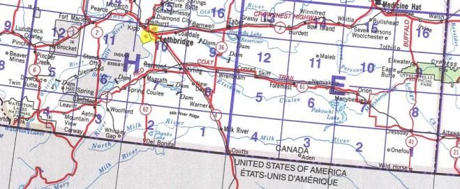
Managing Spatial Data                 December 2013

     GIS IN ECOLOGY:
      MANAGING
     SPATIAL DATA
Introduction
This is an applied course for those with previous
experience using ESRI’s ArcGIS software who want
to acquire and manage spatial data available from
Canadian online sources; e.g. Framework, CanVec,
CDED, Landcover, etc. GIS project development
issues relevant to working with digital spatial data in
ArcGIS are examined. Hands-on exercises in the
“Tasks” section include finding, preparing (e.g.
converting, combining layers, and projection issues),
and managing data efficiently. You will learn tips and
tricks that you can readily apply when creating your
own custom spatial database.

In a typical GIS analysis project, you need to identify
the objectives of your project, create a project
database containing the data you need to solve the
problem, do any necessary preprocessing to get the
data into useable format for the task at hand, use
GIS functions to create an analytical model to solve
the problem, and finally interpret and present your
results. Acquiring and processing the data can take
more time than necessary (upwards of 80% of GIS
project development) if you don’t have the
appropriate skills to import files, work with various
projections, and basically get all your data “ducks”
lined up on a row. And to make matters more
challenging, some of the spatial data you obtain may
not be GIS-ready or easily interpretable.

ccn@ualberta.ca                                   2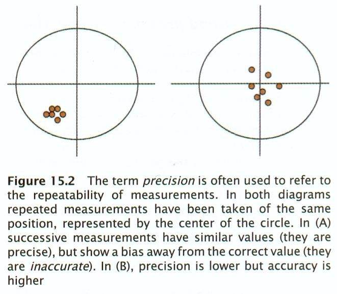
Managing Spatial Data December 2013
Data Acquisition
Tips to keep in mind
Copy the website address for future
reference (e.g. documenting metadata)
Look for readily useable, or easily imported,
file formats
See the ArcGIS Desktop Help topics
Common formats shown in the table
below (and may be zipped archives
*.zip)
Check for projection information – it is very
important that you know the exact datum
and parameters; the data may not be
explicitly defined in the GIS, but with the
proper knowledge you can remedy this
Download (or ask for) metadata – this may
be a simple readme.txt file, MS Word
document *.doc, Excel spreadsheet *.xls,
Adobe Acrobat *.pdf, or *.XML file
In the absence of formal metadata, save (or
print to image or *.pdf) the web page details
File formats
GIS files come in a variety of formats. Common file
types supported by ArcGIS include:
VECTOR
Geodatabase
ESRI Shapefile
ArcInfo coverage
PC ARC/INFO coverage
TIN
DXF, DWG, DGN
RASTER
Geodatabase Raster
ESRI GRID
ERDAS Imagine (.IMG)
Windows Bitmap (.BMP)
JPEG File Interchange Format, JIFF (.JPG)
LizardTech MrSID (.SID)
Tagged Image File Format, TIFF (.TIF)
TABLE
Geodatabase Table
Text file (.TXT, .CSV)
DBASE file (.DBF)
INFO table
The most frequently imported data formats
supported in ArcGIS include the following:
OUTPUT
INPUT FORMAT FORMAT
Atlas Geo file (.AGF) ESRI
MapInfo Interchange Format (.MIF) Shapefile
ArcInfo export interchange file (.E00)
ArcInfo
Spatial Data Transfer Standard SDTS
coverage
Point Profile (.TVP)
Spatial Data Transfer Standard SDTS ESRI
Raster Profile (RSDF, LDEF) GRID
ccn@ualberta.ca 3
Managing Spatial Data December 2013
ASCII
US Digital Terrain Elevation Data
(DTED)
USGS Digital Elevation Model (.DEM)
Data Management
Once you acquire your digital data, maintaining an
organized database is key to effective analysis.
Getting your data “ducks” lined up in a row may
involve several activities in both the management
and preparation (next section). The following are
some recommendations for managing GIS data file
structures, specifically naming conventions, backup
suggestions, and metadata practices:
HANDY TIP
Always keep a notebook with you beside your
computer to jot down notes on sources (e.g.
website) of your data, informal metadata, details on
any processing you perform, information on useful
help files, step-by-step instructions on the analyses
you execute to answer your research question(s),
etc.
Naming conventions
Decide on a concise (short), descriptive (but not
too long) naming convention in the beginning,
and stick to it; this may include:
Using general common sense names or
specialized names as appropriate
Study area abbreviations as prefixes – it
may be hard to keep track of multiple
streams or roads datasets when combining
data from different geographic regions
Projection abbreviations as suffixes – when
starting out with managing GIS data,
sometimes you may want to adopt the ‘over-
kill’ practice of suffixing _nad83z12 at the
end of your datasets, just to keep it all
straight
Date worked on – for example, use
yyyymmdd as the prefix or suffix of a
dataset, especially when digitizing a
complete coverage that may take several
days to complete
Version – add this to the end of the filename
if you’re carrying out multiple edits
throughout the day
Do NOT use spaces in any of the file names –
including the directory paths (this is mostly a
consideration when working with raster data, but
it’s just a good rule of thumb) – instead use the
underscore character “_”
Backup suggestions
Be sure to keep your current work readily available
(in case of the dreaded hard drive crash or errors in
ccn@ualberta.ca 4
Managing Spatial Data December 2013
processing that may be found days later) by backing
it up to an alternate storage device; e.g. server,
secondary/external hard drive, CD/DVD or at
minimum a separate location on your single hard
drive. The following are two suggestions for doing
so:
Backup Method 1: Create a new working
directory/gdb each day you work on your
database
Name with today’s date and the project
name; e.g. yyyymmdd_projname1
Copy ALL files from the previous day’s work
into the new directory/gdb
Backup Method 2: Use an archiving program to
ZIP each day’s work into a new file
At the end of each working day, zip up the
entire working directory and save it using a
filename with today’s date and the project
name; e.g. yyyymmdd_projname1.zip
Continue working on the main directory/gdb,
but create new zip at the end of each day
Delete previous backup files from several days ago
to “declutter” your drive.
Metadata practices
Document your data files from the moment you
acquire them!
ArcCatalog can facilitate this very nicely. Use
the built-in metadata editor to write in the
important characteristics of each dataset so that
future use (by you or others) will know the
history and particulars about the data.
Some useful references on metadata include the
following:
ArcGIS Desktop Help topic: Working with
metadata
Federal Geographic Data Committee
(FGDC): http://www.fgdc.gov/metadata
ESRI Profile of the Content Standard for
Digital Geospatial Metadata:
http://downloads.esri.com/support/whitepapers/a
o_/GeospatialMetadataProfile_J8709_3-03.pdf
Metadata and GIS:
http://downloads.esri.com/support/whitepapers/a
o_/metadata-and-gis.pdf
Data Preparation Issues
Projecting to matching coordinate systems –
ArcMap has the ability to reproject on-the-fly
allowing different layers to line up. However, some
tools and operations may yield unexpected results
when you use them. It is always a good idea to have
all your layers in the same coordinate system and
defined (e.g. *.prj for shapefiles).
ccn@ualberta.ca 5Managing Spatial Data December 2013 Aggregating similar features – Some datasets (e.g. CanVec) contain a wealth of spatial information in multiple layers. Combining them into single layers based on similar geographic features (points, lines, polygons) makes them easier to work with, especially when symbolizing and reprojecting. Exploring and symbolizing layer files – Getting to know the attributes associated with your layers helps you to unleash the power of the geospatial data. Think of the GIS as a database that understands geometry. Tables of data can be linked together and joined to feature classes or raster datasets if they share a common attribute or ID. Through symbology, you can communicate specific attributes of your geographic information by making the map look more visually appealing and convey more meaningful information. ArcMap has several ways to spruce up legend styles to help describe how the data is displayed. You can then conveniently save everything about the layer (symbology, labels, classification) as a layer file (i.e. *.lyr) that when added to another map document will reference the data source and tell ArcMap to draw it exactly as it was saved. Documenting metadata - Metadata is the all- important ancillary information associated with a GIS layer or coverage that characterizes the data set content, quality, condition and other characteristics, and generally includes: date of production, name of creator, data type (raster or vector), instrument type, coordinate system: projection and datum (very important), subject content, attributes (a.k.a. database fields), minimum mapping unit or cell size (scale/resolution), and much more… A helpful practice is to always document this information in a standardized way so that at a later date you or someone else can make sense of it all and know how to appropriately use the data for GIS analyses. You may take advantage of ArcCatalog’s metadata tools or implement your own system using commonly available software, such as MS Excel or MS Access. ccn@ualberta.ca 6
Managing Spatial Data December 2013 Tasks Your overall goal is to set up a GIS project database for the Milk River area in southern Alberta where you may be researching a particular plant community, aquatic system, wildlife phenomenon, or other ecological question. Copying the Course Dataset 1. Double click on the COURSES shared directory icon on the Desktop 2. Open the “GIS-100” folder (double click on it) 3. Select and copy the “7_MSD” folder (right click and choose Copy) 4. Click on the FOLDERS icon along the top menu bar 5. On the left side of the exploring window, click and drag the scroll bar until you can see “My Computer” 6. Expand/open “My Computer” and “Local Disk (C:)” by clicking on the “+”s 7. Paste in the C:\WorkSpace (right click and choose Paste) 8. Once all the files have copied over, close the exploring window 9. To use the ArcGIS Online base map and imagery service, you will need to AUTHENTICATE for internet access Creating the Database There are three basic steps for acquiring pre- existing GIS data: Establish required data needs (where/what) Find and order/download Make all the data ‘GIS-ready’ (unzip/import) Initiating the database Create two new file geodatabases for storing your intermediate and final data files: ccn@ualberta.ca 7
Managing Spatial Data December 2013
1. Start ArcCatalog and navigate to the
C:\Workspace \7_MSD folder
2. SHOW ArcToolbox, if needed
3. In ArcToolbox, click DATA MANAGEMENT
TOOLS >>> WORKSPACE >>> CREATE
FILE GDB
Specify the File GDB Location: \7_MSD
Type File GDB Name: Work - this will
store your intermediate work
Click OK
4. REPEAT to create the MilkRiver.gdb - this
will store your final data layers
5. Explore the various folders of available files
A great starting point in acquiring your digital
data is to determine the geographic extent.
From there you can brainstorm on the nature of
data needed to address your research/mapping
needs. Index maps provide a useful search
‘tool’ when identifying your region of interest
because they provide the often needed
information for when you order/download your
files.
For more information on the National
Topographic System (NTS) see:
http://maps.nrcan.gc.ca/topo101/index_e.php
NTS map sheets are defined by up to three
elements:
a number (1:1,000,000)
one of 16 letters (1:250,000)
a number 1 to 16 (1:50,000)
Determining your study area
6. Start a new empty ArcMap map document
7. SHOW ArcToolbox, if needed
8. Click the ADD DATA button
9. Navigate to \7_MSD\IndexMaps.gdb and
add the following feature classes:
nts_snrc50k
utm
10. Navigate to \7_MSD\Framework1M and
add ALL layer files
11. Navigate to \7_MSD\ArcGISOnline and add
the following layers:
World_Imagery.lyr
World_Physical_Map.lyr
World_Street_Map.lyr
World_Topographic_Map.lyr
TIP: Use the layers in \Framework1M and
\ArcGISOnline folders for your own
research!
12. ZOOM IN on southern Alberta and locate
the Milk River study area through
ccn@ualberta.ca 8Managing Spatial Data December 2013
visualization and inspection of the attributes
for the various reference layers
13. In the table of contents, turn on/off each of
the layers to view
14. Use the IDENTIFY tool and OPEN
ATTRIBUTE TABLE for each to learn which
NTS map sheets and UTM zones include
the Milk River
How many 1:50,000 NTS map sheets cover
the study area? How many UTM zones?
15. When viewing attribute tables, click the
SELECTED button to show those records
16. Set the DATA FRAME >>> COORDINATE
SYSTEM tab to an appropriate projection
for the study area (HINT: NAD 1983 UTM
Zone ?)
17. Use the SELECT FEATURES tool to
interactively select the 1:50,000 scale NTS
index map tiles that completely cover the
Canadian portion of the river basin
18. In the table of contents, right-click
nts_snrc50k and choose DATA >>>
EXPORT DATA
Click to Use the same coordinate
system as the data frame
Save the Selected Features as
\Work.gdb\nts_utm12
19. Optionally, in the attribute table view click
OPTIONS >>> EXPORT to save the table
to a file that can be opened in a text editor
or MS Excel (this is handy for future transfer
of information, say listing the map sheets
you need to download/order, or passing on
to a government agency that may be
providing you with additional data)
Now, prepare a study area extent polygon
to be used for clipping other data layers.
20. In ArcToolbox, choose DATA
MANAGEMENT TOOLS >>>
GENERALIZATION >>> DISSOLVE
Input Features: nts_utm12
Output Features: extent
Click OK
Optionally, create an extent polygon in the
original geographic coordinate system. You
never know if you’ll need a study area layer
that’s unprojected! Once you have established
where and what types of data you need, check
out the various free online web resources and
also contact the UofA Library staff
knowledgeable about academic licensed spatial
data services. Contacting government agencies
may also be needed.
ccn@ualberta.ca 9Managing Spatial Data December 2013
Acquiring selected data sources
Use the lists of index map identifiers to help you
locate and download/order your data. For a
listing of useful Alberta & Canada websites,
please see:
www.biology.ualberta.ca/facilities/gis/?Page=2980
Specific data files already downloaded for this
short course are as follows (NOTE: original
downloads of data are stored in the \DATA
folder, and selected metadata have been saved
to the _documentation folder):
DATA FILES WEB SOURCE
IndexMaps.gdb http://geogratis.cgdi.gc.ca/geogratis/en
/download/topographic.html
C:\Program Files\ArcGIS\Reference
Systems\utm.shp
\Framework1M http://geogratis.cgdi.gc.ca/geogratis/en
/download/framework.html
\ArcGISOnline http://help.arcgis.com/en/arcgisonline/a
golbasemaps.html
World_Imagery.lyr,
World_Physical_Map.lyr,
World_Street_Map.lyr,
World_Topographic_Map.lyr
\DATA\CanVec http://geogratis.cgdi.gc.ca/geogratis/en
/download/topographic.html
\DATA\CDED http://www.geobase.ca/geobase/en/dat
a/cded/
\DATA\GSC http://geoapps.nrcan.gc.ca/applications
\DATA\NLWIS http://www4.agr.gc.ca/AAFC-
AAC/display-
afficher.do?id=1227635802316&lang=
eng
TIP: The NLWIS Landcover product covers the
agricultural region of Canada. Other land cover and
classification products for Canada can be accessed
through GeoGratis, GeoConnections, or SAFORAH
(e.g. CFS EOSD landcover is useful for forested
study areas).
See the Appendix on FTP – this is a most
efficient method for mass downloading! Upon
receiving the files, examine each of the data
products to help you decide if they are indeed
appropriate for your research. If you cannot
immediately view the data then you must import
or convert them to the proper formats.
Unzipping
To unzip files is a cinch using ZipGenius/WinZip
or similar utility. First look at the original files in
Windows Exploring and then determine which
needs extraction by unzipping:
1. Start Windows Exploring
2. Navigate to the C:\WorkSpace\7_MSD
directory
ccn@ualberta.ca 10Managing Spatial Data December 2013
3. Explore each of the sub-folders to see what
they contain
4. Extract the archived data files as
demonstrated – write down notes!
5. Consult the HELP if you are unfamiliar with
this utility
6. Unzip ALL *.zip files into their respective
originating folders then inspect/examine
them
Make note of the file format (coverage,
shapefile, raster), geographic extent,
subject matter, projection information
(especially datums) and other important
metadata for each of the datasets. You’ll
need to know where to quickly find this info
when processing the various datasets. Also,
inspect and examine the files from within
ArcCatalog where you can explore and
visualize the data, and then directly address
any processing requirements using
ArcToolbox (next sections below).
7. In ArcCatalog’s catalog tree, navigate to
C:\WorkSpace\7_MSD\DATA
8. Click the “+” to expand each of the folders
9. Select any one of the layers and click on the
PREVIEW tab to preview the GEOGRAPHY
and TABLE (see drop-down list below the
display window)
10. Right click on one of the layers
11. Choose PROPERTIES
12. Review the information contained here and
close the window when done
13. Right Click on another layer select Item
Description and examine the METADATA -
do all layers have ‘complete’ information
here?
14. PREVIEW all the other data layers in the
subfolders of C:\WorkSpace\7_MSD
15. Go back to the CONTENTS tab for the
\7_MSD\GSC directory
Importing an interchange file (.E00)
Select ArcToolbox - Conversion Tools – To
Coverage, Select Import from E00 and double
click. Each tool is a wizard-driven interface in
which you select the input file, specify the
output name, and enter any associated
parameters. The import tools work in similar
ways.
16. Click on the browse button (looks like an
opening folder)
17. Navigate to the input file and select one;
e.g. \7_MSD\DATA\GSC\GEO1880A.E00
18. Click OPEN
ccn@ualberta.ca 11Managing Spatial Data December 2013
19. Click on Output Folder and select the GSC
directory, click Add
20. In the Output name space type geo1880a
21. Click OK – you will now have a vector
coverage named geo1880a
Projecting
Data often need to be projected to your study
area coordinate system, and it may take more
than one step depending on the original and
target systems. All data seem to be in the GCS
NAD1983 coordinate system, except: CanVec
(GCS_North_American_1983_CSRS), NLWIS
(GCS_WGS_1984), and GSC. The latter data
requires an intermediate projection and a
transformation:
1. In ArcToolbox choose DATA
MANAGEMENT TOOLS >>>
PROJECTIONS AND
TRANSFORMATIONS >>> FEATURE >>>
PROJECT geo1880a\polygon to NAD
1927 UTM Zone 12 and save as
\Work.gdb\geo1880a_n27
2. PROJECT geo1880a_n27 to NAD 1983
UTM Zone 12 (remember the NTV2
transformation) and save as
\Work.gdb\geo1880a_n83
NOTE: You already did some projecting when
you created your nts_utm12 polygon!
Preparing/Customizing Data
Topographic Features from CanVec
CanVec is a digital database of topographic
features developed for all of Canada. ArcGIS
can directly read and analyze the available GIS-
ready file formats, which in this course are the
shapefiles (i.e. required extensions *.shp,
*.shx, *.dbf). Each geographic feature comes in
its own shapefile. Aggregating the similar types
(points, lines, polygons) greatly facilitates
management and symbolizing of this data.
1. Start a new empty ArcMap map document
2. In ArcCatalog, navigate to
\7_MSD\DATA\CanVec
3. While ArcCatalog is also open and both
ArcMap and ArcCatalog windows are
viewable onscreen, select ALL shapefiles
from each subfolder
4. Click and drag to add to the ArcMap data
frame (select all, then click and drag from
each subfolder in ArcCatalog to the Data
ccn@ualberta.ca 12Managing Spatial Data December 2013
View window [NOT the table of contents!] in
ArcMap)
5. In ArcCatalog, click on the CanVec folder
and then choose VIEW >>> REFRESH
6. Minimize ArcCatalog
Notice how ArcMap automatically organizes the
layers by feature type – points, lines polygons.
When working with numerous shapefiles like
this, it is more convenient to group the layers by
feature type (points, lines, polygons) and then
move them to their own data frames to facilitate
merging into well-ordered themes.
Notes about CanVec
Both 1:250,000 and 1:50,000 data are
available
Individual NTS mapsheet tiles are
available as shapefiles
Entire provinces or country are available
as file gdb!
7. Holding the CTRL key, click any of the
checks (within a check box in table of
contents)
8. Select all the point feature layers (click on
the first one then while holding the SHIFT
key, click on the last one)
9. Right click on one of the highlighted layers
10. Choose GROUP
11. Rename this layer as “points”
12. Collapse the group layer by clicking the “-”
13. REPEAT the grouping for the “lines” and
“polygons” (and rename the grouped layers
as indicated and collapse)
14. Optionally, save each grouped layer as a
layer file
While they are not symbolized in any special
way, the advantage of having the grouped
features as layer files gives you the flexibility of
adding the layer files to a new map document
for future work (and in the event of a computer
crash) without having to add from each of the
individual folders again.
15. INSERT two new data frames – choose
INSERT >>> DATA FRAME
16. Click and drag the “lines” grouped layer to
one of the new data frames
17. Remove the original from the first data
frame
18. Click and drag the “polygons” grouped
layer to the other new data frame
19. Remove the original from the first data
frame
ccn@ualberta.ca 13Managing Spatial Data December 2013
This might seem overboard in the
organization department, but it certainly
beats having to pick through all feature
types when you want to merge certain
layers in the next few steps. You may also
go one step further and save as layer files.
20. Optionally, double click on EACH data
frame and set the COORDINATE SYSTEM
to NAD 1983 UTM ZONE 12 (set the correct
transformation method, too)
21. SAVE the map document; e,g,
CanVecGroups.mxd
22. Right click on the data frame containing
“points” and choose ACTIVATE
Explore some of the data layers to get a feel for
what can be combined and what you want kept
separate. For example, the *_TO_*.shp files
should be combined with only each other to
create a complete coverage across all map
sheets. All other point features can be
aggregated and then symbolized/selected by
the THEME field. READ the files in the
\_documentation folder to learn more about
what the names and attributes mean. Don’t you
agree that using numeric codes is pretty smart
for a bilingual country?
READ the documentation -
CanVec_feature_catalogue_en.pdf - to learn
more about what the names and attributes
mean.
Now, to keep all output layers in the same
coordinate system as the one chosen for your
study area, it's more efficient to set this as a
global environment setting.
23. Click on Geoprocessing in the menu and
choose ENVIRONMENTS
24. In the ENVIRONMENT SETTINGS
category:
Set the workspaces to the \Work.gdb
Set Output Coordinate System to ‘As
Specified Below’ >>> NAD 1983 UTM
Zone 12
Set the transformation to
NAD_1983_To_NAD_1983_CSRS_3
Click OK
25. Choose DATA MANAGEMENT TOOLS >>>
GENERAL >>> MERGE
26. Select ALL *_TO_*.shp files - easiest to
select in the TOC and drag to the input
window
27. Type an output name; e.g.
\Work.gdb\toponames
28. Click OK
ccn@ualberta.ca 14Managing Spatial Data December 2013
29. Remove the old *_TO_*.shp files from the
group layer
30. Repeat the MERGE for all other point
features to create a new \Work.gdb\points
– the THEME field can be used for future
mapping and analysis queries
31. ACTIVATE the data frame containing
“lines”
The water features and contours should
also be kept separate from other entity
types when merged. Human access
features – roads, rail, pipelines, etc. – may
be combined. Remove each set of layers
after they have been merged to help with
the next selection of layers to process.
Read the documentation to learn more
about what the names and attributes mean.
TIP: The CanVec_Codes_v1_1 table,
available in the \IndexMaps.gdb, is similar to
CanVec_EntitiesCodesFileNames_EntitesC
odesNomsDeFichier_v1_1_0.xls.
32. MERGE each theme for the various linear
features, save all to \Work.gdb, and
remember to remove the highlighted layers
from the table of contents each time (this
reduces the number of files to sort through):
all single line watercourses (HD) and
name it watercourses
all contour lines (FO_1030009) and
name it contours
all human linear types (everything else)
and name it linear – highlight one of the
TR_1760009 layers and click the UP
ARROW button to set this as the
topmost input layer; this will require the
output to retain all the road attributes,
which is more numerous than the other
line features
33. ACTIVATE the data frame containing
“polygons”
34. Save all polygon outputs to \Work.gdb
35. MERGE each theme for the various linear
features, save all to \Work.gdb, and
remember to remove the highlighted layers
from the table of contents each time (this
reduces the number of files to sort through):
all hydro polygon files (HD_1480009)
into \Work.gdb\waterbodies_Merge
all wetland polygon files (SS_1320049)
into \Work.gdb\wetlands_Merge
aggregate one or two others of interest;
e.g. wooded_Merge (VE_1240009)
Because ArcToolbox’s global environment was
set to output the same coordinate system as
ccn@ualberta.ca 15Managing Spatial Data December 2013
the display (data frame), the merge output is
automatically reprojected to NAD83 UTM. Now
you have newly created feature classes
projected in the coordinate system of choice to
analyze and map for the Milk River project
database. Note: Merging polygons is not always
a good idea because the merge operation
results in a “sandwich” layer effect of
overlapping polygons. You must carefully
consider the input order or opt to use union
instead when aggregating polygon features!
The next step is to generalize the data between
the map sheet edges.
36. ACTIVATE the data frame containing
“polygons”
37. Choose DATA MANAGEMENT TOOLS >>>
GENERALIZATION >>> DISSOLVE
Select waterbodies as the input
features
Specify \Work.gdb\waterbodies as the
output feature class
Check both THEME and
PERMANENCY as the Dissolve Fields
Uncheck ‘Create multipart features’
Click OK
38. REPEAT dissolving by THEME (check for
any other fields?) for the wetlands,
vegetation, etc. and save in the \Work.gdb
39. Reset ArcToolbox's ENVIRONMENTS to
default values - a very good idea, especially
when switching between projects
Canadian Digital Elevation Data
You can download national coverage DEMs in
1:250,000 (~90 meter) and 1:50,000 (~20
meter) scales. Canadian Digital Elevation
Data (CDED) is digital terrain data available in
USGS DEM format from Natural Resources
Canada (NRCan). ArcGIS can read, import, and
export the single file type (*.dem). The following
procedures outlines the steps necessary for
mosaicking and reprojecting (DO take a closer
look at the help for each of the parameters and
pay attention to the # of bands and bit depth):
1. In a new empty ArcMap, add all the *.dem
files to visualize how the tiles appear
2. In ArcToolbox, choose DATA
MANAGEMENT TOOLS >>> RASTER
>>>RASTER DATA SET>>> MOSAIC TO
NEW RASTER
Select ALL available rasters as the Input
Rasters
ccn@ualberta.ca 16Managing Spatial Data December 2013
Specify Output Location:
\7_MSD\Work.gdb
Type the Raster dataset name:
dem_gcs
Click OK
Now it is time to project the data into the study
area’s chosen map projection:
3. Choose DATA MANAGEMENT TOOLS >>>
PROJECTIONS AND
TRANSFORMATIONS >>> RASTER >>>
PROJECT RASTER
4. Specify the:
Input raster: dem_gcs
Output raster: dem_utm
Output coordinate system:
NAD_1983_UTM_Zone_12N
Output cell size: 20
5. Click OK
You now have one seamless layer of CDED
data projected to NAD 1983 UTM Zone 12. You
may wish to choose a different coordinate
system to suit your particular study area when
applying these instructions to another dataset,
or even “clip” your data to fit a smaller study
area boundary.
Surficial geology from GSC
The Geological Survey of Canada (GSC) data
is at a 1:5,000,000 scale and is useful for
practicing the tasks of joining attribute tables,
projections, and clipping. This particular dataset
is a digital version of the surficial geology of
Canada map. You have already projected it,
now you will populate the attribute table and
subset to the study area extent.
1. Start a new empty ArcMap map document
2. ADD the projected geo1880a_n83 from the
\Work.gdb (NAD 1938 UTM Zone 12)
3. OPEN ATTRIBUTE TABLE for
geo1880a_n83
4. In Windows Exploring, locate the
information (HINT: \_documentation) you
need to interpret the codes in the
GEOPOLY field
5. Back in ArcMap, ADD DATA: geopolye.xls
6. Double click on geo1880a_n83 polygon to
access its Layer Properties
7. In the JOINS & RELATES tab, click ADD in
the Joins frame (left side)
8. Choose to join the GEOPOLY field to the
geopolye.xls table’s GEOPOLY field
9. Click OK twice
ccn@ualberta.ca 17Managing Spatial Data December 2013
10. Examine the joined attribute table and
optionally, symbolize using one of the joined
fields
11. In the Layer properties’ FIELDS tab, check
off any of the unwanted fields (e.g. click the
CLEAR ALL button and check on
GEOPOLY, GEOMOD, Label, and
Description
12. Click OK and view the table with its reduced
number of columns
13. ADD DATA: extent from the Work.gdb
14. Open the CLIP tool and specify the
following parameters:
Input Features: geo1880a_n83
Clip features: extent
Output Feature Class:
\Work.gdb\surfgeol
15. Click OK
Take a few moments to reflect on all the
processing performed and notice the few minor
tricks incorporated (join by attributes, turn
unwanted fields off) to extract the desired data
for the study area. NOTE: This 1:5M scale data
is likely too coarse for this study area.
Landcover from NLWIS
The National Land and Water Information
System (NLWIS) is part of Agriculture and Agri-
Food Canada. Their thematic land cover map
was produced through remote sensing
classification of Landsat satellite imagery from
circa 2000. The 30 meter data cover the Milk
River study area.
1. In a new empty map document or data
frame, ADD DATA from \Work.gdb: extent
2. ADD DATA from the \DATA\NLWIS folder:
lcv_utm12_aafc_30m_2000_v11.tif
3. CLIP / EXTRACT BY POLYGON /
EXTRACT BY MASK the landcover layer to
just the study area extent subset and save
as \Work.gdb\landcover
4. CHALLENGE: Assign descriptive
names/labels to the subset raster attribute
table
More data?
If time, examine the metadata and files for the
NRN and SLC directories to process, subset to
extent, and add these datasets to the study
area database.
ccn@ualberta.ca 18Managing Spatial Data December 2013
Copy to Final Database
1. Import/export/copy all the final layers
(feature classes and rasters that have been
aggregated, projected to NAD 1983 UTM
Zone 83, and/or subsetted by clip/extract) in
to the MilkRiver.gdb
Use ArcCatalog to right-click on
MilkRiver.gdb and choose IMPORT >>>
Or in ArcToolbox choose
CONVERSION TOOLS >>> TO
GEODATABASE >>> … (multiple)
2. CHALLENGE: Use ArcCatalog or MS
Excel/MS Access to create metadata
documentation describing the original data
files, the processing you performed, and
properties of your final dataset layers in the
\MilkRiver.gdb directory
For example, in MS Excel/MS Access set up
column headings for a table that indicate the
original input layers complete with descriptions
of content, file format, file location, extent,
scale, coordinate system/datum, source, etc.,
and the final output layers complete with the
same information, along with the processing
details that generated them. See Chapter 9 in
the Using_ArcCatalog.pdf for documenting
metadata in ArcGIS. Metadata is very useful!!!
What next?
What you do with your data depends on your
research objectives. To get you this far, you
already determined what kinds of data were
needed to meet your objectives as identified by
your GIS project development. Now that you’ve
completed the acquisition and preparation you
are ready to apply the appropriate GIS
functions and methods to analyze the data and
produce the output products you need. Other
tutorials and short courses can help you
address these issues.
Appendix A: Brief Notes on
Scale, Accuracy, and
Precision
You may have noticed the spatial differences
among the various data sets – this is due to the
variation in source methods and scale. The
producers of each dataset created the data for
specific purposes, which may have required
ccn@ualberta.ca 19Managing Spatial Data December 2013 generalization of features to fit the appropriate scale of mapping/analysis (as well as other sources of error). This leads to an interesting issue regarding scale as a property of the digital database. The definition of scale (ratio of distance in the computer map to distance on the ground) makes no sense to digital data because how can there be distances in a computer? When scale is quoted for a digital database it usually means the scale of the map that formed the source of the digital data. The scale of data capture (digitizing, remote sensing, GPS, etc.) influences the accuracy of the data. When you display the national-level data with the 1:50,000 data, the generalization of the large regional scale is readily apparent: Milk River appears jagged and doesn’t conform to the gentle meanders visible in the finer data. Another important point to remember is that the earth is not a perfect sphere, is in constant motion, and is subject to minute movements from seismic, drift, and wobbling; therefore, accurate measurements on the earth’s surface are inherently uncertain. Do not confuse accuracy with precision, which is often referred to as the repeatability of and number of digits used to report measurements. ccn@ualberta.ca 20 Lon
Managing Spatial Data December 2013
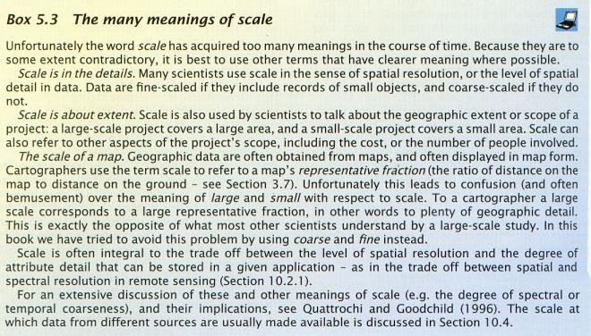
To add to the complexity of scale issues,
spatial scale (e.g. grain size, extent,
representative fraction, minimum mapping unit,
etc.) is not the only matter to be concerned with
when establishing your GIS project database.
Scale also includes temporal and spectral
characteristics. The timing of data capture
affects the temporal scale – very significant
when analyzing time-sensitive phenomena or
for just preserving a proper time frame among
the various data sources (e.g. you wouldn’t
want an airphoto from 1972 when your research
will be performed next summer). In the case of
remote sensing data, spectral scale defines the
wavelengths of electromagnetic radiation – very
affective when differentiating among earth
features (e.g. healthy green vegetation greatly
reflects in the near-infrared wavelengths and
absorbs in the red and blue wavelengths).
Of course, this brief discussion is only the tip of
the iceberg where scale is concerned when
compiling your GIS database. Excellent
selected references for further reading are
listed below:
Environmental Systems Research Institute, Inc. 1995-
2010. ArcGIS Desktop Help.
Environmental Systems Research Institute, Inc. 1995-
2010. ESRI Virtual Campus.
http://campus.esri.com/
Lillesand, T.M. and Kiefer, R.W. 2000. Remote sensing
and Image Interpretation. John Wiley & Sons,
Toronto, Ontario.
Longley, P.A., Goodchild, M.F., Maguire, D.J., and Rhind,
D.W. 2001. Geographic Information Systems
and Science. John Wiley & Sons, Ltd.
Chichester UK.
National Center for Geographic Information and Analysis
(NCGIA). 2007. GIS Core Curriculum.
http://www.ncgia.ucsb.edu/education/curricula/cct
p/Welcome.html
…and so many more…
Note: When “mixing” datasets of various
scales, your output will only be as spatially
accurate as the coarsest scale!
Appendix B: FTP Information
When you need to download many files in many
directories, it is more efficient to use a File
Transfer protocol application, such as the
following highly recommended free and open
source:
ccn@ualberta.ca 21Managing Spatial Data December 2013
http://filezilla-project.org
You may also use the AICT provided clients, which
have online documentation on their use, from here:
http://helpdesk.ualberta.ca/storage/filetransfer.html
Log on as anonymous with your email for the
password.
The main hosts are ftp2.cits.rncan.gc.ca and
ftp.geogratis.gc.ca and ftp.agr.gc.ca:
Typically, inside the \pub directory are all the
publicly available spatial data products from
NRCan. You may need to type in the
subdirectory (subfolder) name; e.g.
\geobase\cded.
You can expand your local site and navigate to
the directory folder you wish to download files
to – and also create new directories within.
Then simply select, click, and drag from the
remote side (NRCan directories) to your local
hard drive!
Appendix C: Very Useful
ArcGIS Online Resources
http://support.esri.com
http://help.arcgis.com/en/arcgisdesktop/10.0/help/ind
ex.html
http://resources.arcgis.com/content/product-
documentation?fa=viewDoc&PID=17&MetaID=10
03 (PDFs of older manuals)
http://resources.arcgis.com/en/home/
ccn@ualberta.ca 22You can also read