Ghost City Extraction and Rate Estimation in China Based on NPP-VIIRS Night-Time Light Data - MDPI
←
→
Page content transcription
If your browser does not render page correctly, please read the page content below
International Journal of
           Geo-Information

Article
Ghost City Extraction and Rate Estimation in China
Based on NPP-VIIRS Night-Time Light Data
Wei Ge 1 , Hong Yang 1,2, *, Xiaobo Zhu 1 , Mingguo Ma 1, *     ID
                                                                     and Yuli Yang 3
 1    Chongqing Engineering Research Center for Remote Sensing Big Data Application, School of Geographical
      Sciences, Southwest University, Chongqing 400715, China; godwin6@email.swu.edu.cn (W.G.);
      wavelet@email.swu.edu.cn (X.Z.)
 2    Department of Geography and Environmental Science, University of Reading, Reading RG6 6AB, UK
 3    School of civil engineering, Lanzhou University of Technology, Lanzhou 730050, China; yyl1980111@lut.cn
 *    Correspondence: hongyang@gmail.com (H.Y.); mmg@swu.edu.cn (M.M.); Tel.: +86-23-6825-3912 (M.M.)

 Received: 3 May 2018; Accepted: 13 June 2018; Published: 15 June 2018

 Abstract: The ghost city phenomenon is a serious problem resulting from the rapid urbanization
 process in China. Estimation of the ghost city rate (GCR) can provide information about vacant
 dwellings. This paper developed a methodology to quantitatively evaluate GCR values at the
 national scale using multi-resource remote sensing data. The Suomi National Polar-Orbiting
 Partnership–Visible Infrared Imaging Radiometer (NPP-VIIRS) night-time light data and moderate
 resolution imaging spectroradiometer (MODIS) land cover data were used in the evaluation of the
 GCR values in China. The average ghost city rate (AGCR) was 35.1% in China in 2013. Shanghai had
 the smallest AGCR of 21.7%, while Jilin has the largest AGCR of 47.27%. There is a significant
 negative correlation between both the provincial AGCR and the per capita disposable income of urban
 households (R = −0.659, p < 0.01) and the average selling prices of commercial buildings (R = −0.637,
 p < 0.01). In total, 31 ghost cities are mainly concentrated in the economically underdeveloped inland
 provinces. Ghost city areas are mainly located on the edge of urban built-up areas, and the spatial
 pattern of ghost city areas changed in different regions. This approach combines statistical data with
 the distribution of vacant urban areas, which is an effective method to capture ghost city information.

 Keywords: China; VIIRS night-time light; ghost city; vacant urban area

1. Introduction
     China has experienced rapid urbanization in the last decades [1]. Between 1978 and 2012, China’s
urban population increased from 12.9 to 52.6% [2]. The National Plan on New Urbanization, which was
issued in March 2014, is a macroscopic, strategic and fundamental plan in China. This plan elaborates
a set of urbanization targets for China to be achieved by 2020, transforming national urbanization
into a people-oriented and ecologically friendly new type of urbanization. However, China’s rapid
urbanization process has produced some serious problems, for example environmental degradation
and a waste of resources [3–5]. The ghost city phenomenon is a serious problem, has had severe
effects on land use and ecosystems, creating a waste of energy and resources [4,6]. To promote the new
urbanization process, the Chinese ghost city problem should be resolved.
     There are some studies on ghost cities [7,8]. The problem was first reported and named by
the western media. In 2010, Time magazine published a group of pictures of Ordos City in Inner
Mongolia [9]. Despite many buildings in the city, no lights were lit at night, earning its status as a
“ghost city”. Since then, China’s ghost city problem has been reported frequently in the world’s major
media outlets. However, the term “ghost city” is not clearly defined. Shepard [10] defined “ghost
city” as “a new development that is running at severe under-capacity, a place with drastically fewer

ISPRS Int. J. Geo-Inf. 2018, 7, 219; doi:10.3390/ijgi7060219                       www.mdpi.com/journal/ijgi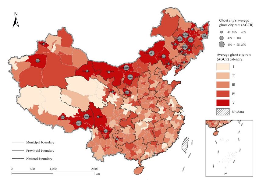
ISPRS Int. J. Geo-Inf. 2018, 7, 219                                                                  2 of 17

people and businesses than there is available space for.” Moreover, the ghost city in China is not
caused by natural or human-caused disasters such as floods, prolonged droughts, pollution, war or
nuclear disasters, but caused by the faster expansion of urban land than the growth of the urban
population, which results in few or no inhabitants in urban areas. The Chinese ghost city phenomenon
is a unique characteristic of China’s rapid urbanization [11]. Thus, there lack of similar ghost city cases
to Chinese ghost cities, which are caused by the differences between the urban land expansion and
urban population growth. In this study, a ghost city is defined as a municipal region where the vacant
built-up area phenomenon is most serious (Section 3.3). We extracted the ghost cities using the degree
of vacancy.
      Some simple extraction methods for Chinese ghost cities have been proposed in previous studies.
The Ministry of Housing and Urban Rural Development of the People’s Republic of China indicates that
the standard urban population density should be 10,000/km2 . According to this standard, the standard
ranking organization defined one half of the above standard as the ghost city threshold. In 2015,
this organization released China’s ghost city index list, which includes 50 cities. Chi et al. [12] used
location and population data for research into ghost cities. Jin et al. [10] combined news coverage, road
data and the Defense Meteorological Satellite Program–Operational Linescan System (DMSP-OLS)
stable night-time data to identify China’s ghost cities. However, the extraction results for vacant areas
in ghost cities lack spatial pattern information. Zheng [11] used the NPP-VIIRS cloud mask product,
multi-source land cover data, and population data to identify ghost cities at the county level. However,
the temporal resolution of the data was different (2010 and 2013), and the analysis did not take into
account the influence of the Chinese Spring Festival. During this period (from January to March),
a large portion of the urban population returned to their hometowns, and the ghost city phenomenon
appeared in large cities for a short time.
      The housing vacancy rate is one of the most important indicators for assessing the health status of
urban real estate. The Ministry of Housing and Urban Rural Development of the People’s Republic
of China issued an urban planning and construction standard indicating that residential land should
account for 25–40% of urban construction. In the urban built-up area, the main land coverage is
residential land. In addition, housing is the main type of residential land. However, there are no official
statistics on the housing vacancy rate in China. The China Household Finance Survey (CHFS) [13]
found that the urban housing vacancy rate was quite high, with a rapid increase from 20.6% in 2011
to 22.4% in 2013. Yao et al. [14] studied the Chinese housing vacancy rate with DMSP-OLS stable
night-time light data. Chen et al. [15] used NPP-VIIRS night-time light data and high resolution land
use data to estimate the housing vacancy rate in the United States with good results. According to
international standards, a housing vacancy rate between 5 and 10% is normal [16], which means that
the real estate market can allow house vacancy for some time. Based on the above study, we accepted
the hypothesis that a ghost city area is part of an urban built-up area that has a vacancy phenomenon.
      Night-time light imagery can be a good representation of human socio-economic activity [17–19].
This imagery is widely used in urbanization monitoring [20], population estimates [21–23], major
disaster monitoring [24,25] and ecological assessment [26,27]. Urban light is the main source of
land night-time light [25]. The use of night-time light data can be successfully applied to urban
expansion studies [26–32]. Therefore, the NPP-VIIRS night-time light and moderate resolution imaging
spectroradiometer (MODIS) land cover data were selected for the extraction of China’s ghost cities.
This study had two main objectives: (1) to develop a methodology for estimating China’s ghost city
rate; and (2) to obtain the distribution and morphological characteristics of the ghost cities in China.

2. Materials and Methods
    In this paper, 31 provincial administrative regions and 333 prefecture-level administrative regions
in China with different levels of urbanization and socioeconomic development were selected as the
study area.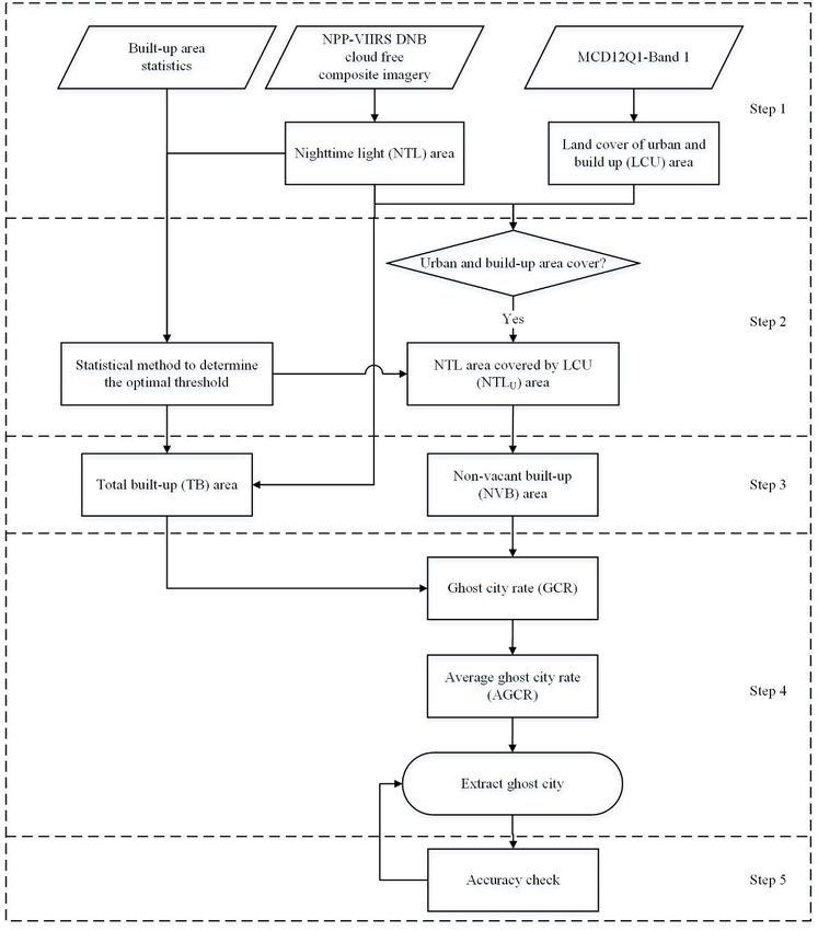
ISPRS Int. J. Geo-Inf. 2018, 7, 219 3 of 17
2.1. Data
ISPRS Int. J. Geo-Inf. 2018, 7, x FOR PEER REVIEW 3 of 17
The night-time light data used in this paper comprise the NPP-VIIRS day and night band (DNB)
2.1. Data
cloud-free composite imagery, obtained from the National Oceanic and Atmospheric Administration
The night-time
(NOAA) [33]. light data
The NPP-VIIRS DNBused in this paper
cloud-free comprisenight-time
composite the NPP-VIIRS lightday and night
imagery wasband (DNB)
post-processed
cloud-free composite imagery, obtained from the National Oceanic and Atmospheric Administration
to remove clouds and correct for stray light [34]. These data are monthly composites with a spatial
(NOAA) [33]. The NPP-VIIRS DNB cloud-free composite night-time light imagery was post-
resolution of 15 arc seconds (approximately 462.5 m). In this study, the December 2013 NPP-VIIRS
processed to remove clouds and correct for stray light [34]. These data are monthly composites with
DNBanight-time light data
spatial resolution of 15 was selected
arc seconds to extract the462.5
(approximately urban
m).built-up area.the
In this study, The December
December 2013night-time
NPP-
light VIIRS
data DNB
can reflect the final expansion of urban built-up areas and population
night-time light data was selected to extract the urban built-up area. The December night-distribution in
2013.time light data can reflect the final expansion of urban built-up areas and population distribution in
Compared to another commonly-used stable night-time light dataset, the DMSP-OLS [35–37],
2013. Compared
the NPP-VIIRS DNB to composite
another commonly-used
imagery hasstable beennight-time
calibrated light
in dataset, the DMSP-OLS
orbit, providing [35–37],
a higher spatial
the NPP-VIIRS
accuracy and solving DNBthecomposite
brightnessimagery has been
saturation calibrated
problem in orbit,
[34,38]. providing
However, a higher
these spatial not
data contain
only accuracy and solving
the brightness from theurban
brightness
areassaturation
but alsoproblem [34,38].
abnormal valuesHowever,
such asthese
firedata contain
points, not only and
volcanoes
background noise. Figure 1 shows that the NPP-VIIRS DNB data contains some pixels with and
the brightness from urban areas but also abnormal values such as fire points, volcanoes negative
background noise. Figure 1 shows that the NPP-VIIRS DNB data contains some pixels with negative
values, which are caused by data compositing. In addition, the original data also contain some
values, which are caused by data compositing. In addition, the original data also contain some
abnormal pixels with extremely large values, a phenomenon associated with highly reflective surfaces.
abnormal pixels with extremely large values, a phenomenon associated with highly reflective
Thesesurfaces.
abnormal Thesevalues would
abnormal interfere
values wouldwith the extraction
interfere process. process.
with the extraction Due toDue the to
above problems,
the above
problems, the original NPP-VIIRS DNB night-time light data had to be corrected.
the original NPP-VIIRS DNB night-time light data had to be corrected.
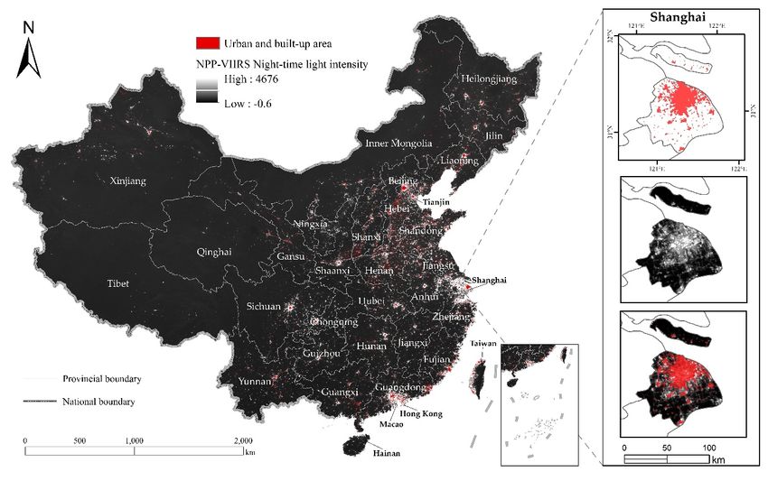
Figure
Figure 1. TheSuomi
1. The Suomi National
NationalPolar-Orbiting
Polar-OrbitingPartnership–Visible InfraredInfrared
Partnership–Visible Imaging Radiometer (NPP-
Imaging Radiometer
VIIRS) imagery
(NPP-VIIRS) imagerynight-time light
night-time from
light December
from December20132013
and and
MODIS land land
MODIS covercover
type type
yearly data data
yearly
(MCD12Q1,
(MCD12Q1, 2013)2013) urban
urban andand built-upareas
built-up areasfrom
from 2013,
2013, and
andzoomed
zoomedinin Shanghai.
Shanghai.
The combined MODIS land cover type yearly data (MCD12Q1, 2013) were obtained from the
United
The States Geological
combined MODISSurvey (USGS)type
land cover [39]. yearly
The MCD12Q1 land cover data
data (MCD12Q1, have
2013) a spatial
were resolution
obtained from the
of 500
United m, Geological
States as shown inSurvey
Figure 1. It employs
(USGS) [39].the
TheInternational
MCD12Q1 Geosphere–Biosphere
land cover data haveProgram
a spatial(IGBP)
resolution
classification
of 500 m, as shown scheme, and the
in Figure 1. 13th class comprises
It employs urban and built-up
the International areas, indicating land
Geosphere–Biosphere covered
Program (IGBP)
by buildings and other man-made structures.
classification scheme, and the 13th class comprises urban and built-up areas, indicating land covered
The and
by buildings China Statistical
other man-made Yearbook is an annual statistical publication compiled by the National
structures.
Bureau of Statistics in China, including economic and social statistics for the past year. Data on the
The China Statistical Yearbook is an annual statistical publication compiled by the National
urban built-up areas in the 31 provincial administrative regions in 2013 [40] were used in this study.
Bureau of Statistics in China, including economic and social statistics for the past year. Data on the
urban built-up areas in the 31 provincial administrative regions in 2013 [40] were used in this study.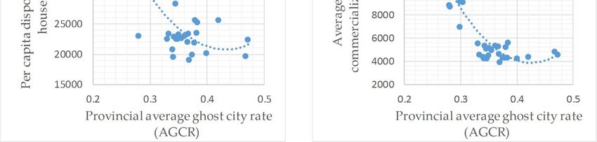
ISPRS Int. J. Geo-Inf. 2018, 7, 219                                                                                       4 of 17

2.2. Methods
     ISPRS Int. J. Geo-Inf. 2018, 7, x FOR PEER REVIEW                                                              4 of 17

     In
      2.2.summary,
            Methods the proposed approach in this study includes five steps (Figure 2). The first step is
the remote sensing data preprocessing phase, in which the night-time light (NTL) data and urban and
             In summary, the proposed approach in this study includes five steps (Figure 2). The first step is
built-up land cover (LCU) data are resampled and re-projected. The second step is to extract the NTLU ,
      the remote sensing data preprocessing phase, in which the night-time light (NTL) data and urban
in which
      and the    NTLland
            built-up    areas   are covered
                              cover (LCU) databyareLCU    areas. At
                                                      resampled       there-projected.
                                                                    and    same time,The the second
                                                                                             optimal    threshold
                                                                                                     step            for built-up
                                                                                                           is to extract  the
area extraction     is determined       by the  built-up    area   statistics and   NTL   area.  The
      NTLU, in which the NTL areas are covered by LCU areas. At the same time, the optimal threshold  third   step  is to for
                                                                                                                           use the
optimal    threshold
      built-up          to extractisthe
                 area extraction          built-up by
                                       determined     area
                                                         theinbuilt-up
                                                                the NTL    and
                                                                        area     NTLUand
                                                                              statistics data.
                                                                                             NTLThese
                                                                                                   area.two
                                                                                                          Theresults    represent
                                                                                                               third step   is
the total
      to usebuilt-up   (TB)threshold
               the optimal     area andtothe   actual
                                            extract theurban
                                                         built-uparea  with
                                                                    area      non-vacant
                                                                         in the NTL and NTL built-up
                                                                                                U data.(NVB)     areas.
                                                                                                         These two        The last
                                                                                                                     results
      represent
step is            the total
        to calculate      thebuilt-up  (TB)rate
                                ghost city   area (GCR)
                                                  and theandactual  urban
                                                                  the       area with
                                                                      average    ghost non-vacant
                                                                                         city rate built-up
                                                                                                    (AGCR)(NVB)        areas. the
                                                                                                                and extract
      The
ghost city. last step  is  to  calculate the ghost   city  rate  (GCR)   and  the  average  ghost  city  rate (AGCR)     and
       extract the ghost city.

                               Figure 2. Workflow of the ghost city extraction and rate estimation.
                           Figure 2. Workflow of the ghost city extraction and rate estimation.
       2.2.1. Night-Time Light and Land Cover Data Preprocessing
2.2.1. Night-Time Light and Land Cover Data Preprocessing
            As discussed in Section 2.1, most of the background noise has been removed in the original NPP-
    VIIRS
    As     DNB monthly
        discussed        night-time
                  in Section        light of
                              2.1, most   imagery, but some abnormal
                                             the background          values
                                                             noise has beenstill remain,inincluding
                                                                            removed         the original
NPP-VIIRS DNB monthly night-time light imagery, but some abnormal values still remain, including
negative values and extremely large values. The negative values are caused by the monthly imagery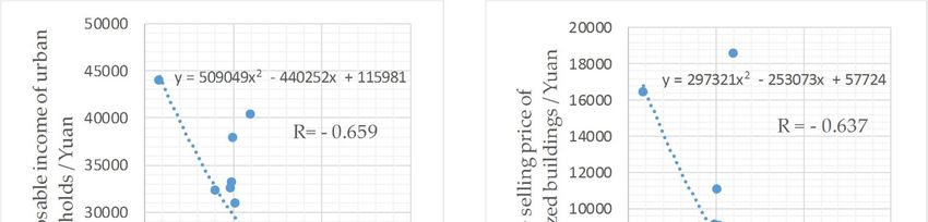
ISPRS Int. J. Geo-Inf. 2018, 7, 219                                                                5 of 17

composition process and were regarded as background noise in this study. Thus, we removed this
background noise and set the minimum threshold of the NTL imagery to 0. When correcting the
NPP-VIIRS DNB data to extract the built-up area, the maximum brightness of the central urban area
can be equal to the maximum threshold of the NTL data [41]. The city with the highest gross domestic
product (GDP) in 2013 was Shanghai. As such, we treat Shanghai as the most developed region in
China in 2013. Therefore, we use the maximum light intensity (294.349 nWcm−2 sr−1 ) of Shanghai’s
central built-up area as the maximum threshold for all NTL pixels in China. After this process, the NTL
data were in the range of 0–294.349. The land cover data in the MCD12Q1-band1 dataset used the
IGBP classification scheme. The 13th land cover class was extracted to retrieve the urban and built-up
land cover (LCU) area.
     All remote sensing data were projected into the Albers conical equal area projection, and the
nearest neighbor algorithm was used to resample to keep the pixel size at 500 m by 500 m.

2.2.2. Determine the Built-Up Area Extraction Threshold and Extract NTLU
      The built-up area with night-time light data was extracted in two strategies: imagery segmentation
and constructing the feature space [28,42]. The construction of the feature space was generally
characterized by combining the night-time light data and the Vegetation Index (VI) or other high
spatial resolution remote sensing products, but this method had a high dependence on high-resolution
data [43–47]. Considering the large scale in this study, the imagery segmentation method was
employed. During the process to extract the urban built-up area based on the night-time light data
using the imagery segmentation method, it is important to determine the optimal threshold. Previous
studies have developed a number of methods using the optimal threshold techniques [20,27,43,45–48].
      The statistical data method was used to determine the light intensity threshold using statistical
data on the built-up area that had been published by many government departments due to
its relatively high accuracy and reliability [42]. Specifically, the optimal extraction threshold was
determined by dichotomies in the night-time light imagery. When the extracted area was closest to
the total built-up area data, the optimal extraction threshold was determined [20]. The statistical data
method was easy to implement, with a good accuracy and agreement with the NPP-VIIRS night-time
data [27].
      Moreover, due to large regional differences in the geographical environment and socio-economic
development, it was difficult to use a single threshold to extract China’s built-up area [30,48].
We improved the statistical data method for application in this study using statistical data on the
built-up area from 31 provinces and NPP-VIIRS NTL data to calculate the optimal built-up area
extraction threshold. The optimal threshold contains both the maximum threshold and minimum
threshold in this study. The maximum threshold was the maximum light brightness of the most
developed region’s central urban area in a province, and the minimum threshold was set using
statistical data. This process was iterated by increasing the threshold until the extraction area and the
statistical area were the closest. The optimal thresholds for built-up area extraction in China and the
31 provincial administrative regions are listed in Table 1.
      Comparing the LCU area with the NTL data indicates that pixels with high fractional settlements
generally had high DN values in the NTL imagery. The NTL data were fused with LCU to improve
the NVB extraction accuracy and calculate the NTLU , the areas where the NTL areas were covered by
LCU areas. It can be extracted using overlay analysis.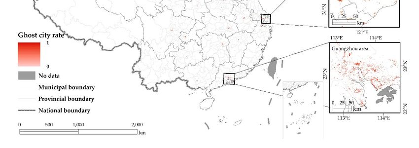
ISPRS Int. J. Geo-Inf. 2018, 7, 219                                                                                                                                      6 of 17

      Table 1. Built-up areas and extraction thresholds. The areas of the built-up districts were from the 2013 China Statistical Yearbook. The built-up area extraction
      thresholds were determined by the statistical data method.

                                                            Minimum          Maximum                                                     Minimum            Maximum
                                      Area of Built-Up                                                            Area of Built-Up
    ID          Area Name                                   Threshold        Threshold      ID     Area Name                             Threshold          Threshold
                                       Districts (km2 )                                                            Districts (km2 )
                                                          (nWcm−2 sr−1 )   (nWcm−2 sr−1 )                                              (nWcm−2 sr−1 )     (nWcm−2 sr−1 )
     1           China                   47,855.28            23.109          294.349       17      Jiangsu             3809.6             20.113              269.941
     2           Anhui                    1777.26             16.219          115.588       18       Jiangxi           1151.42              9.806              178.601
     3           Beijing                  1306.45             18.972          268.765       19         Jilin           1344.02             10.295              218.771
     4         Chongqing                  1114.92              9.92            120.46       20     Liaoning            2386.49             12.175              282.241
     5           Fujian                   1263.18             22.771          124.431       21      Ningxia             420.69             18.401              144.833
     6           Gansu                     726.66             13.268          139.574       22      Qinghai             157.36             19.065               87.485
     7         Guangdong                  5232.11             17.074          290.252       23      Shaanxi             915.02             25.896              227.707
     8          Guangxi                   1153.64             13.813           94.626       24     Shandong            4187.48             11.284              261.585
     9          Guizhou                     695.4             18.163          137.207       25     Shanghai             998.75             32.321              294.349
    10           Hainan                    296.03             19.133           84.273       26       Shanxi            1040.69              18.95              132.119
    11           Hebei                    1787.24             14.297           89.186       27      Sichuan            2058.11             13.901              175.011
    12           Henan                    2289.08             13.861          291.556       28       Tianjin            747.26             25.855              253.574
    13        Heilongjiang                1758.38             11.747          249.615       29        Tibet             120.29             12.659              153.719
    14           Hubei                    2006.71             10.862          275.906       30      Xinjiang           1064.87             23.108              132.259
    15           Hunan                    1504.95             11.794          183.506       31      Yunnan              935.77             20.977              222.083
    16       Inner Mongolia               1206.21             14.607          196.655       32      Zhejiang           2399.24             18.487              293.636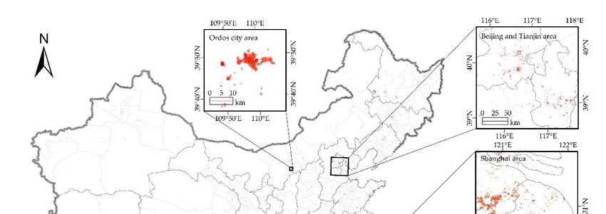
ISPRS Int. J. Geo-Inf. 2018, 7, 219                                                                  7 of 17

2.2.3. Extracting Total Built-Up Area and Non-Vacant Built-Up Areas
      Due to the difference in spatial resolution and algorithms, the MCD12Q1 data are very different
with respect to the spatial extent of China’s built-up areas [11]. In addition, the built-up area from the
MCD12Q1 was found to be larger than the official statistical data. Due to of these issues, the LCU data
from the MCD12Q1 dataset cannot be used to extract the TB directly. Moreover, the official statistics
include the real area of the built-up areas in China. Thus, the statistical data method was used to
extract the TB area. More details were mentioned in Section 2.2.2.
      The NVB is the area of active human habitation. A large population and frequent socio-economic
activities in these areas were indicated by high brightness. Therefore, the NVB satisfies two conditions:
it has built-up area land cover, and the light intensity is greater than a certain threshold (the minimum
threshold shown in Table 1). The optimal extraction threshold and the NTLU data were used to extract
the NVB.
      The statistical data on built-up areas determines the quantitative area characteristics, the land
cover data determines the spatial distribution characteristics. The NVB data both satisfy the quantitative
area characteristics and land cover spatial distribution characteristics. The optimal threshold was
used to extract the NTL and NTLU , respectively, and obtain the TB and NVB accordingly. The TB was
extracted from the built-up area statistics and NTL data, and the NVB were extracted from the NTLU
data and optimal threshold.

2.2.4. Calculating the Ghost City Rate and Statistical Analysis

                                                          NVBi
                                           GCRi = 1 −                                                   (1)
                                                           TBi
where GCRi is the vacancy intensity of the ith pixel in a ghost city area. NVBi and TBi are the light
intensity values of the ith pixel in the NVB and TB, respectively.
     To improve the comparability and visual accuracy of the GCR, the seriousness of the ghost city
phenomenon was described in different administrative regions. The GCR imagery was used in this
research to generate a new ghost city index with a linearly weighted average algorithm, as expressed in
Equation (2). The average ghost city rates (AGCR) at both the provincial and municipal administrative
scales were calculated.
                                                   ∑n     GCRi f i
                                         AGCR = i = n1                                              (2)
                                                      ∑i = 1 f i
where AGCR is the average ghost city rate of the administrative regions; GCRi is the GCR of the ith pixel
in an administrative region; f i is the number of the GCRi pixel and n is the nth administrative region.
     Moreover, to explore the factors influencing ghost cities in China, correlation analyses between
the provincial AGCR and several indicators were conducted using SPSS 19 (Statistical Product and
Service Solutions, IBM, Armonk, NY, USA).

2.2.5. Accuracy Check
      He et al. [20] used the statistical method to extract the built-up areas on a provincial scale and had
good extraction results (accuracy error less than 3%). However, considering that the statistical data
method is a threshold extraction method, the different scales of the built-up area statistical data may
have influenced the extraction results. This difference may affect the extraction results of ghost cities.
Due to the above issue, an accuracy check was conducted. The same workflow diagram (Figure 2)
of this study was used to estimate the AGCR on a smaller scale using the municipal built-up area
statistical data. The five cities were selected as samples to carry out this work. The five sample cities
included two capital cities, Hohhot (the capital city of Inner Mongolia) and Xi’an (the capital city of
Shaanxi) and three cities with the low municipal AGCRs, Songyuan (a city in Jilin), Hengyang (a city
in Hunan), Hanzhong (a city in Shaanxi). The statistical data on the built-up area of the five sample
cities were derived from the statistical bulletins and work reports of the local governments in 2013.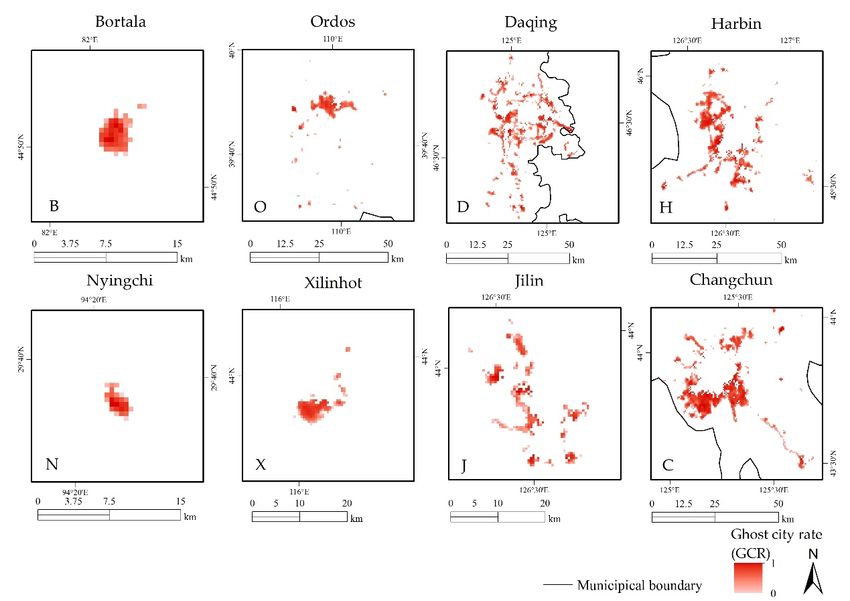
ISPRS Int. J. Geo-Inf. 2018, 7, x FOR PEER REVIEW                                                          8 of 17

in Hunan), Hanzhong (a city in Shaanxi). The statistical data on the built-up area of the five sample
 ISPRS were
cities Int. J. Geo-Inf.
               derived  2018, 7, 219
                           from                                                                             8 of 17
                                   the statistical bulletins and work reports of the local governments in 2013.

3. Results
3. Results
3.1.
3.1. Ghost
     GhostCity
           CityRate
               RateEstimation
                    Estimation
      After
       After the
              the above
                  above five
                         five steps,
                              steps, raster
                                      raster imagery
                                              imagery of
                                                       of the
                                                           the GCR
                                                               GCR in
                                                                    in China
                                                                       China was
                                                                             wascreated
                                                                                 created (Figure
                                                                                          (Figure 3).
                                                                                                  3). Each
                                                                                                      Eachpixel
                                                                                                           pixel
represents    an  area of 0.25  km2 2, and the pixel value is the proportion of the vacancy, which ranges
 represents an area of 0.25 km , and the pixel value is the proportion of the vacancy, which ranges from
from
 0 to 10and
         to 1reflects
              and reflects  the seriousness
                      the seriousness    of theofghost
                                                  the ghost  city phenomenon.
                                                       city phenomenon.

      Figure 3.
     Figure     Spatial distribution
             3. Spatial distributionof
                                     ofChina’s
                                       China’sghost
                                               ghostcity
                                                     city rate
                                                           rate in
                                                                 in 2013.
                                                                    2013. The
                                                                          Thefour
                                                                              fourregions
                                                                                   regionsare
                                                                                          are magnified
                                                                                              magnified and
                                                                                                        and
      shown  in detail.
     shown in detail.

     Four
      Four cities
             citieswere
                    wereselected
                         selectedtoto show
                                        show thethe
                                                  changes  from
                                                     changes      NTL
                                                               from    to GCR
                                                                      NTL      in the
                                                                           to GCR   in extraction  process.
                                                                                        the extraction       The
                                                                                                          process.
results are  shown   in Figure   4. In Harbin,   the  capital city of Heilongjiang  Province,   the
The results are shown in Figure 4. In Harbin, the capital city of Heilongjiang Province, the AGCR wasAGCR    was
52.32%.
 52.32%. In
          InChangchun,
             Changchun,the thecapital
                                capitalcity
                                         cityof
                                              ofJilin
                                                 Jilin Province,
                                                       Province, the
                                                                  the AGCR
                                                                      AGCR was
                                                                             was 55.28%.
                                                                                 55.28%. In In Shanghai,
                                                                                               Shanghai,oneone of
                                                                                                               of
China’s
 China’s four
          four municipalities,
                municipalities, the
                                 the provincial
                                     provincial AGCR
                                                 AGCR was was 21.75%.
                                                              21.75%. In
                                                                       In Changsha,
                                                                          Changsha, the
                                                                                      the capital
                                                                                          capital city
                                                                                                  city of
                                                                                                       ofHunan
                                                                                                           Hunan
Province,
 Province, the
            the AGCR
                 AGCR was
                        was 40.12%.
                            40.12%.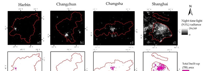
ISPRS Int. J. Geo-Inf. 2018, 7, 219 9 of 17
ISPRS Int. J. Geo-Inf. 2018, 7, x FOR PEER REVIEW 9 of 17
Figure
Figure 4. Four
4. Four different
different spatial
spatial distributionsofofthe
distributions theestimated
estimatednight-time
night-time light
light (NTL),
(NTL), total
totalbuilt-up
built-up (TB)
area (TB)
and area
ghostand
cityghost
rate city
(GCR) ratein(GCR) in four cities.
four typical typicalThe
cities.
a1,The
b1, a1, b1, c1
c1 and d1and
are d1
theare the NPP-VIIRS
NPP-VIIRS night-time
lightnight-time
radiance;light
a2, radiance;
b2, c2, and a2, b2,
d2 c2,
areand
thed2total
are the total built-up
built-up areasthe
areas and andoptimal
the optimal threshold;
threshold; a3,a3,b3, c3,
b3, c3, and d3 are ghost city rate imagery. The red lines in figures are the municipal administrative
and d3 are ghost city rate imagery. The red lines in figures are the municipal administrative boundaries.
boundaries.
3.2. Provincial Average
3.2. Provincial Ghost
Average City
Ghost CityRate
Rateand
and Correlation Analysis
Correlation Analysis
Using Equation
Using Equation(2),(2),
thetheAGCR
AGCRof of 31 provincialadministrative
31 provincial administrative regions
regions werewere calculated
calculated (Table(Table
2). 2).
Provinces with a high AGCR were Jilin, Heilongjiang, Inner Mongolia and Tibet. The
Provinces with a high AGCR were Jilin, Heilongjiang, Inner Mongolia and Tibet. The regions withregions with
AGCRs
AGCRs less than
less than 30% 30% included
included Shanghai,
Shanghai, Tianjin,
Tianjin, Jiangsu,
Jiangsu, Guangdong,
Guangdong, Hainan
Hainan and
and Beijing.The
Beijing. Thelowest
lowest AGCR was found in Shanghai,
AGCR was found in Shanghai, only 21.71%. only 21.71%.
Table 2. AGCR of China and 31 provincial administrative regions.
Table 2. AGCR of China and 31 provincial administrative regions.
ID Region Name AGCR (%) ID Region Name AGCR (%)
ID 1Region China
Name 35.1(%) 17 ID Jiangsu
AGCR Region Name 29.81 AGCR (%)
1 2 China Anhui 35.04
35.1 18 17 Jiangxi Jiangsu 36.7 29.81
2 3 Anhui Beijing 32.07
35.04 19 18 Liaoning Jiangxi 38.01 36.7
3 4 Beijing
Chongqing 38.44
32.07 20 Inner
19 Mongolia
Liaoning42.06 38.01
4 5 Chongqing
Fujian 30.35
38.44 21 20 Ningxia 37.89
Inner Mongolia 42.06
5 6 FujianGansu 30.35
36.92 22 21 Qinghai Ningxia 34.2 37.89
6 7 Gansu
Guangdong 36.92
29.91 23 22 ShandongQinghai 34.57 34.2
7 8 Guangdong
Guangxi 29.91
36.84 24 23 Shanxi Shandong34.92 34.57
8 9 Guangxi
Guizhou 36.84
34.05 25 24 Shaanxi Shanxi 34.26 34.92
9 Guizhou 34.05 25 Shaanxi 34.26
10 Hainan 28.1 26 Shanghai 21.71
10 Hainan 28.1 26 Shanghai 21.71
11 Hebei 35.55 27 Sichuan 33.09
11 Hebei 35.55 27 Sichuan 33.09
12 12 Henan Henan 34.74
34.74 28 28 Tianjin Tianjin 28.06 28.06
13 13Heilongjiang
Heilongjiang 46.76
46.76 29 29 Tibet Tibet 40.01 40.01
14 14 Hubei Hubei 36.18
36.18 30 30 Xinjiang Xinjiang37.45 37.45
15 15 Hunan Hunan 38.29
38.29 31 31 Yunnan Yunnan 33.41 33.41
16 Jilin 47.27 32 Zhejiang 30.13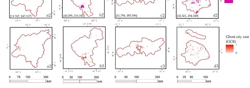
ISPRS
 ISPRS Int.
        Int. J.J. Geo-Inf.
                  Geo-Inf. 2018,
                           2018, 7,
                                 7, xx FOR
                                       FOR PEER
                                           PEER REVIEW
                                                REVIEW                                                               10
                                                                                                                     10 of
                                                                                                                        of 17
                                                                                                                           17
ISPRS Int. J. Geo-Inf. 2018, 7, 219                                                                                   10 of 17
                       16
                       16             Jilin
                                      Jilin          47.27
                                                     47.27     32
                                                               32        Zhejiang
                                                                         Zhejiang              30.13
                                                                                               30.13

      The
      The results
      The  results indicated
           results    indicated that
                     indicated    that there
                                  that   there were
                                        there   were significant
                                                were   significant negative
                                                      significant      negative correlations
                                                                       negative     correlations between
                                                                                    correlations  between the
                                                                                                  between    the provincial
                                                                                                            the  provincial
                                                                                                                  provincial
AGCR
AGCR
AGCR and and   two
         and two     indicators
              two indicators       (Figure
                    indicators (Figure
                                 (Figure 5). 5). The
                                           5). The     first
                                               The first      indicator
                                                   first indicator
                                                          indicator was    was
                                                                       was the    the
                                                                             the per    per
                                                                                  per capitacapita  disposable
                                                                                       capita disposable
                                                                                              disposable income
                                                                                                          income income
                                                                                                                   of     of
                                                                                                                   of urban
                                                                                                                       urban
urban   households.
households.
households.     The      The second
                The second
                       second  indicatorindicator
                                indicator   was
                                            was the was
                                                  the     the average
                                                       average
                                                        average    selling
                                                                    sellingselling
                                                                               priceprice
                                                                              price   of    of commercialized
                                                                                      of commercialized
                                                                                         commercialized           buildings.
                                                                                                            buildings.
                                                                                                            buildings.   The
                                                                                                                         The
The  Pearson
Pearson         correlation
Pearson correlation           coefficients
           correlation coefficients
                           coefficients were   were  −
                                           were −0.659 0.659
                                                 −0.659 (p      (p <  0.01)
                                                            (p
ISPRS Int. J. Geo-Inf. 2018, 7, 219 11 of 17
Table 3. The AGCR classification by the standard deviation (STD) method. The AGCR is the average
ghost city rate; AGCRi is the AGCR of the ith municipal region; AGCRmax and AGCRmin are the
maximum and minimum municipal AGCR values, respectively; m is the mean; and std is the standard
deviation of the 333 municipal AGCRs in China.
AGCR Category Division Standard Result of Division Count Percentage
I AGCRmin ≤ AGCRi < m − std 0 ≤ AGCRi < 22.56% 38 11.41%
II m − std ≤ AGCRi < m − 0.5 std 22.56% ≤ AGCRi < 26.97% 41 12.31%
III m − 0.5 std ≤ AGCRi < m + 0.5 std 26.97% ≤ AGCRi < 35.78% 164 49.25%
IV m + 0.5 std ≤ AGCRi < m + std 35.78% ≤ AGCRi < 40.18% 59 17.72%
V m + std ≤ AGCRi ≤ AGCRmax 40.18% ≤ AGCRi ≤ 55.35% 31 9.31%
3.4. Accuracy Check
As shown in Table 4, according to the accuracy check of the above five cities, despite the
differences between provincial and municipal scales, the ghost city categories remain consistent.
The municipal AGCR of categories IV and V, for example Hohhot and Xi’an, were overestimated,
where the municipal AGCR of categories I and III, for example Songyuan, Hengyang and Hangzhou,
were slightly underestimated. Thus, the cities with low municipal AGCRs may have a more serious
ghost city phenomenon. The municipal AGCR of category V showed a very small difference (0.06%),
the difference was too small to influence the ghost city extraction. Thus, our ghost city extraction
method is effective when using the provincial-level built-up area statistical data.
Table 4. The difference between the municipal AGCR estimate results using provincial and municipal
built-up area statistical data.
Using Provincial Built-Up Area Using Municipal Built-Up Area
Statistical Data Statistical Data
Validation City Difference (%)
Municipal AGCR (%) Category Municipal AGCR (%) Category
Hohhot 40.25 V 40.19 V 0.06
Xi’an 36.6 IV 35.81 IV 0.79
Songyuan 33.09 III 33.27 III −0.18
Hengyang 28.12 III 30.79 III −2.67
Hanzhong 15.79 I 18.95 I −3.16
At present, there is neither a widely accepted ghost city extraction method nor officially-released
statistics for China. Due to the lack of available ghost city validation datasets, ghost city validation
work is often controversial. Nonetheless, in this research, strong efforts were made to compare the
results with third party institutions, existing papers and media publications to improve the extraction
accuracy of ghost cities in China.
As addressed in the “Introduction”, the housing vacancy rate is one of the most important
indicators for assessing the inhabitant quantity and urban vacancy phenomenon. The CHFS carried
out a sampling survey on the housing vacancy rate across the 29 provinces, 262 counties and
1048 communities in China [13]. They found, on the national scale, that the housing vacancy rates in the
central and western regions were higher than those in the eastern region. On the city scale, the housing
vacancy rates of undeveloped cities were greater than those of the developed cities. According to a
detailed analysis of six cities including Beijing, Shanghai, Chongqing, Chengdu, Wuhan, and Tianjin,
the city with the highest vacancy rates was Chongqing. This is consistent with our results. For instance,
as shown in Figure 6, the ghost cities were mainly concentrated in the economically undeveloped
inland region, and the municipal AGCR of Chongqing (38.44%) was greater than others municipal
cities (Beijing of 32.07% and Shanghai of 21.71%). Moreover, compared with the ghost city extraction
results in previous studies and media reports (Appendix A), most of the previous results showed that
the majority of ghost cities were located in the inland border areas of China, which are consistentISPRS Int. J. Geo-Inf. 2018, 7, 219 12 of 17
ISPRS Int. J. Geo-Inf. 2018, 7, x FOR PEER REVIEW 12 of 17
with our results. Overall, our results using the new effective method are basically consistent with
published
4. results.
Discussion
4. Discussion
4.1. Correlation Analysis on the Provincial Scale
To analyzeAnalysis
4.1. Correlation how the onghost city phenomenon
the Provincial Scale emerged during rapid urbanization in China, a
correlation analysis between the provincial AGCR and two indicators was employed. The per capita
To analyze how the ghost city phenomenon emerged during rapid urbanization in China,
disposable income of urban households is representative of a resident’s purchasing power. The
a correlation analysis between the provincial AGCR and two indicators was employed. The per capita
average selling price of commercialized buildings, calculated by dividing the total price of all
disposable income of urban households is representative of a resident’s purchasing power. The average
commercial buildings by the total area, is an important price index in the real estate market. The
selling price of commercialized buildings, calculated by dividing the total price of all commercial
results showed some useful information, indicating that regions where the residents have weak
buildings by the total area, is an important price index in the real estate market. The results showed
purchasing power and where there are low housing prices always have a serious ghost city
some useful information, indicating that regions where the residents have weak purchasing power and
phenomenon. Areas with high AGCRs are concentrated in the border areas in northeast, northwest
where there are low housing prices always have a serious ghost city phenomenon. Areas with high
and southwest China (Figure 7) and the AGCR in the southeastern coastal areas is relatively low. The
AGCRs are concentrated in the border areas in northeast, northwest and southwest China (Figure 7) and
difference in AGCR from the southeast coast to the northwest inland regions was similar to the
the AGCR in the southeastern coastal areas is relatively low. The difference in AGCR from the southeast
regional differences in economic development. During urban expansion, the levels of urbanization
coast to the northwest inland regions was similar to the regional differences in economic development.
are closely correlated to levels of economic development [38]. In general, the income level of urban
During urban expansion, the levels of urbanization are closely correlated to levels of economic
residents and housing prices are determined by the level of a city’s economic development, which is
development [38]. In general, the income level of urban residents and housing prices are determined
the result of long-term development.
by the level of a city’s economic development, which is the result of long-term development.
Figure 7. The spatial distribution of China’s municipal AGCRs. The five categories of municipal AGCR
Figure 7. The spatial distribution of China’s municipal AGCRs. The five categories of municipal
are shown in the different colors. The 31 ghost cities are labeled with a gray circle with three categories.
AGCR are shown in the different colors. The 31 ghost cities are labeled with a gray circle with three
categories.
4.2. Spatial Pattern of Ghost City Areas
4.2. Spatial
Eight Pattern
typical of Ghost
ghost City(Figure
cities Areas 8) in the eastern (D, J, H, C), central (O, X) and western (B, N)
regions were
Eight selected
typical ghostforcities
comparison.
(Figure 8)By
incomparing
the easternthese
(D, J,typical
H, C), ghost
centralcities,
(O, X)we could
and see that
western (B, the
N)
ghost city
regions areas
were in different
selected cities haveBy
for comparison. their own spatial
comparing patterns.
these Ghostcities,
typical ghost city areas in thesee
we could developed
that the
ghost city areas in different cities have their own spatial patterns. Ghost city areas in the developed
eastern coastal cities were more dispersed, showing a round or ring shape, while in undeveloped
central and western areas, ghost city areas were aggregated, showing an oval shape.ISPRS Int. J. Geo-Inf. 2018, 7, 219 13 of 17
eastern coastal cities were more dispersed, showing a round or ring shape, while in undeveloped
ISPRS Int.and
central J. Geo-Inf.
western 7, x FOR
2018,areas, PEERcity
ghost REVIEW
areas
were aggregated, showing an oval shape. 13 of 17
Figure
Figure 8.
8. Different
Different spatial
spatial patterns
patterns of
of eight
eight ghost
ghost cities,
cities, four
four in
in eastern
eastern China
China (D,
(D, Daqing,
Daqing, AGCR
AGCR is is
46.22%;
46.22%; J,
J, Jilin,
Jilin, AGCR
AGCR isis 40.9%;
40.9%; H,
H, Harbin,
Harbin, AGCR
AGCR is is 52.23%;
52.23%; C,C, Changchun,
Changchun, AGCR
AGCR isis 55.35%),
55.35%), two
two in
in
central
central China
China (O,(O,Ordos,
Ordos,AGR
AGRisis47.16%;
47.16%;X,X,Xilinhot,
Xilinhot, AGCR
AGCR is is
46.94%), and
46.94%), twotwo
and in western China
in western (B,
China
Bortala, AGCR is 41.32%; N, Nyingchi, AGCR is 47.26%); and the black lines in the figures
(B, Bortala, AGCR is 41.32%; N, Nyingchi, AGCR is 47.26%); and the black lines in the figures are the are the
municipal
municipal administrative
administrative boundaries.
boundaries.
Some characteristics were observed in the spatial distribution of ghost city areas. The ghost city
Some characteristics were observed in the spatial distribution of ghost city areas. The ghost city
areas were located on the edges of the built-up areas (Figure 4). In general, the cities’ central areas
areas were located on the edges of the built-up areas (Figure 4). In general, the cities’ central areas had
had well-developed infrastructure, a fast-moving and convenient traffic system, and a high
well-developed infrastructure, a fast-moving and convenient traffic system, and a high population;
population; however, the edges of the urban built-up areas lacked these supportive conditions [6].
however, the edges of the urban built-up areas lacked these supportive conditions [6]. The ghost
The ghost city phenomenon that emerged during the rapid urbanization is due to the urban
city phenomenon that emerged during the rapid urbanization is due to the urban population growth
population growth lagging behind the development of urban land in extreme cases, resulting in few
lagging behind the development of urban land in extreme cases, resulting in few or no people living in
or no people living in the new built-up areas. On the one hand, it is hard to expand a city with a small
the new built-up areas. On the one hand, it is hard to expand a city with a small population and low
population and low economic development power; on the other hand, the attraction to such a city is
economic development power; on the other hand, the attraction to such a city is weak and cannot fill
weak and cannot fill the ghost city area’s population vacancy.
the ghost city area’s population vacancy.
In the process of urban development and construction, the expansion of built-up areas is an
In the process of urban development and construction, the expansion of built-up areas is an
inevitable process. However, in this process, policy guidance by the local government plays an
inevitable process. However, in this process, policy guidance by the local government plays an
important role [50,51]. As we mentioned, the ghost city areas are located on the edges of a city’s built-
important role [50,51]. As we mentioned, the ghost city areas are located on the edges of a city’s
up areas. These areas represent the direction of urban expansion. Thus, these areas were usually
built-up areas. These areas represent the direction of urban expansion. Thus, these areas were usually
planned as new development areas in urban planning. However, unrealistic urban planning policy
planned as new development areas in urban planning. However, unrealistic urban planning policy is
is likely to produce a ghost city phenomenon in the urban new areas, such as Ordos.
likely to produce a ghost city phenomenon in the urban new areas, such as Ordos.
5.
5. Conclusions
Conclusions
In
In this
this study, the ghost
study, the ghost city
city rate
rate (GCR)
(GCR) and
and average
average ghost
ghost city rate (AGCR)
city rate (AGCR) were
were analyzed
analyzed toto
quantify the severity of the ghost city problem using night-time light data. Compared with
quantify the severity of the ghost city problem using night-time light data. Compared with mediamedia
reports and other studies on ghost cities, this method combines statistical data with the distribution
of vacant urban areas, and provides a visual approach to help residents, officials and urban planners
to understand the spatial distribution of ghost cities. After the accuracy check, this method can be
considered as an effective method to capture the ghost city information. The results of this studyISPRS Int. J. Geo-Inf. 2018, 7, 219 14 of 17
reports and other studies on ghost cities, this method combines statistical data with the distribution
of vacant urban areas, and provides a visual approach to help residents, officials and urban planners
to understand the spatial distribution of ghost cities. After the accuracy check, this method can be
considered as an effective method to capture the ghost city information. The results of this study show
that China’s average AGCR was 35.1% in 2013. More than one-third of China’s urban built-up areas
have varying degrees of vacancy.
Correlation analyses were conducted for the relationship between provincial AGCRs and two
indicators (the per capita disposable income of urban households and the average selling price of
commercial buildings). The Pearson correlation coefficients were −0.659 (p < 0.01) and −0.637 (p < 0.01),
respectively, indicating that regions where the residents have weak purchasing power and low housing
prices often have a serious ghost city phenomenon. The result also provides a risk assessment for the
government to establish urban planning policy. Cities where the residents have weak purchasing power
and where there are low housing prices should be more careful with urban planning and policymaking.
At the municipal scale, the vast majority of cities in China have ghost city areas, with AGCRs
ranging from 30 to 35%. Using the municipal AGCR, 31 ghost cities were extracted. These ghost cities
were mainly concentrated in the economically underdeveloped inland provinces, such as Heilongjiang,
Inner Mongolia, and Xinjiang.
Regarding the spatial distribution, the ghost city areas were concentrated along the edges of the
urban built-up areas. The spatial pattern of ghost city areas was different in the different regions
of China. The ghost city areas in the developed regions of eastern coastal China were dispersed,
while they were more aggregated in the western undeveloped regions.
Considering the limitation of the validation data, it is valuable to further improve the evaluation
framework by using multi-source data, such as point of interest, location-based service data and high
spatial resolution nighttime light imagery.
Author Contributions: W.G., H.Y. and M.M. conceived and designed the experiments; W.G. performed the
experiments and analyzed the data; W.G., H.Y., X.Z., M.M. and Y.Y. jointly revised the paper.
Acknowledgments: This study was supported by the National Key Technology R&D Program of China (grant
number: 2016YFC0500106), Special Project of Science and Technology Basic Work (grant number: 2014FY210800-5),
the National Natural Science Foundation of China (41771453), the Open Research Fund Program of Chongqing
Engineering Research Center for Remote Sensing Big Data Application, and Open Research Fund Program of
Chongqing Key Laboratory of Karst Environment, Southwest University.
Conflicts of Interest: The authors declare no conflict of interest.
Appendix A. List of Ghost Cities in China
This Study, 2013 Standard Ranking, 2015 Baidu Big Data Lab, 2015 NetEase Property, 2013
Changchun (Jilin) Erlianhaote (Inner Mongolia) Ordos (Inner Mongolia) Ordos (Inner Mongolia)
Harbin (Heilongjiang) Alar (Xinjiang) Tongliao (Inner Mongolia) Hohhot (Inner Mongolia)
Suihua (Heilongjiang) Beitun (Xinjiang) Shenyang (Liaoning) Bayannaoer (Inner Mongolia)
Changdu (Tibet) Altay (Xinjiang) Changchun (Jilin) Erlianhaote (Inner Mongolia)
Jixi (Heilongjiang) Zhangye (Gansu) Hohhot (Inner Mongolia) Zhengzhou (Henan)
Bayannaoer (Inner Mongolia) Suifenhe (Heilongjiang) Weihai (Shandong) Hebi (Henan)
Nyingchi (Tibet) Qinzhou (Guangxi) Binhai New Area (Tianjin) Xinyang (Xinyang)
Ordos (Inner Mongolia) Jiayuguan (Gansu) Nantong (Jiangsu) Yingkou (Liaoning)
Xilinhot (Inner Mongolia) Yumen (Gansu) Dongying (Shandong) Changzhou (Jiangsu)
Daqing (Heilongjiang) Shigatse (Tibet) Taizhou (Jiangsu) Zhenjiang (Jiangsu)
Aksu (Xinjiang) Golmud (Qinghai) Changshu (Jiangsu) Shiyan (Hubei)
Chifeng (Inner Mongolia) Ruili (Yunnan) Jinnan District (Tianjin) Chenggong (Yunnan)
Qingyang (Gansu) Turpan (Xinjiang) Chengdu (Sichuan)
Liangshan (Sichuan) Mishan (Heilongjiang) Wenzhang (Hainan)
Jiamusi (Heilongjiang) Wuzhong (Ningxia) Rizhao (Shandong)
Lhasa (Tibet) Fukang (Xinjiang) Shaoxing (Zhejiang)
Anshan (Liaoning) Yichun (Heilongjiang) Hangzhou (Zhejiang)
Liaoyuan (Jilin) Shizuishan (Ningxia) Qiongzhou (Hainan)
Jiuquan (Gansu) Xilinhaote (Inner Mongolia)
Baicheng (Jilin) Jinchang (Gansu)ISPRS Int. J. Geo-Inf. 2018, 7, 219 15 of 17
Yichun (Heilongjiang) Fangchenggang (Guangxi)
Benxi (Liaoning) Dehui (Jilin)
Yingkou (Liaoning) Donggang (Liaoning)
Chaoyang (Liaoning) Shulan (Jilin)
Bortala (Xinjiang) Kuerle (Xinjiang)
Lanzhou (Gansu) Ordos (Inner Mongolia)
Jilin (Jilin) Hulunbeier (Inner Mongolia)
Siping (Jilin) Lhasa (Tibet)
Ganzi (Sichuan) Huolinguole (Inner Mongolia)
Liupanshui (Guizhou) Weihai (Shandong)
Alashan (Inner Mongolia) Changshu (Jiangsu)
References
1. Chen, M. Evolution and assessment on China’s urbanization 1960–2010: Under-urbanization or
over-urbanization? Habitat Int. 2013, 38, 25–33. [CrossRef]
2. Bai, X.; Shi, P.; Liu, Y. Realizing China’s urban dream. Nature 2014, 509, 158–160. [CrossRef] [PubMed]
3. Liu, Y.; Huang, X.; Yang, H.; Zhong, T. Environmental effects of land-use/cover change caused by urbanization
and policies in southwest China karst area—A case study of Guiyang. Habitat Int. 2014, 44, 339–348. [CrossRef]
4. Yang, H.; Huang, X.; Thompson, J.R.; Bright, R.M.; Astrup, R. The crushing weight of urban waste. Science
2016, 351, 674. [CrossRef] [PubMed]
5. Yang, H.; Huang, X.; Thompson, J.R.; Flower, R.J. Soil pollution: Urban brownfield. Science 2014, 344, 691–692.
[CrossRef] [PubMed]
6. He, G.; Mol, A.P.J.; Lu, Y. Wasted cities in urbanizing China. Environ. Dev. 2016, 18, 2–13. [CrossRef]
7. Jin, X.; Long, Y.; Sun, W.; Lu, Y.; Yang, X.; Tang, J. Evaluating cities’ vitality and identifying ghost cities in
China with emerging geographical data. Cities 2017, 63, 98–109. [CrossRef]
8. Zheng, Q.; Zeng, Y.; Deng, J.; Wang, K.; Jiang, R.; Ye, Z. “Ghost cities” identification using multi-source
remote sensing datasets: A case study in Yangtze river delta. Appl. Geogr. 2017, 80, 112–121. [CrossRef]
9. Ordos, China: A Modern Ghost Town. Available online: http://content.time.com/time/photogallery/0,
29307,1975397,00.html (accessed on 8 November 2016).
10. Shepard, W. Ghost Cities of China; Zed Books: London, UK, 2015.
11. Zhang, L.; Zhao, S.X. Reinterpretation of China’s under-urbanization: A systemic perspective. Habitat Int.
2003, 27, 459–483. [CrossRef]
12. Chi, G.; Liu, Y.; Wu, Z.; Wu, H. Ghost cities analysis based on positioning data in China. Comput. Sci. 2015,
68, 1150–1156.
13. Urban Housing Vacancy Rate and Housing Market Development Trend. Available online: http://chfs.swufe.
edu.cn/xiangqing.aspx?id=900 (accessed on 16 November 2016).
14. Yao, Y.; Li, Y. House vacancy at urban areas in China with nocturnal light data of DMSP-OLS. In Proceedings
of the 2011 IEEE International Conference on Spatial Data Mining and Geographical Knowledge Services,
Fuzhou, China, 29 June–1 July 2011; pp. 457–462.
15. Chen, Z.; Yu, B.; Hu, Y.; Huang, C.; Shi, K.; Wu, J. Estimating house vacancy rate in metropolitan areas using
npp-viirs nighttime light composite data. IEEE J. Sel. Top. Appl. Earth Obs. Remote Sens. 2017, 8, 2188–2197.
[CrossRef]
16. Wang, H.; Chang, C.J. Simulation of housing market dynamics: Amenity distribution and housing vacancy.
In Proceedings of the 2013 Winter Simulations Conference (WSC), Washington, DC, USA, 8–11 December
2013; pp. 1673–1684.
17. Elvidge, C.D.; Baugh, K.E.; Kihn, E.A.; Kroehl, H.W.; Davis, E.R.; Davis, C.W. Relation between satellite
observed visible-near infrared emissions, population, economic activity and electric power consumption.
Int. J. Remote Sens. 1997, 18, 1373–1379. [CrossRef]
18. Keola, S.; Andersson, M.; Hall, O. Monitoring economic development from space: Using nighttime light and
land cover data to measure economic growth. World Dev. 2015, 66, 322–334. [CrossRef]
19. Wang, X.; Ma, M. The luminous intensity of regional ‘night-light’ output can predict the growing volume of
published scientific research by ‘luminaries’ in developing countries. Scientometrics 2016, 110, 1–6. [CrossRef]ISPRS Int. J. Geo-Inf. 2018, 7, 219 16 of 17
20. He, C.; Shi, P.; Li, J.; Chen, J.; Pan, Y.; Li, J.; Li, Z.; Ichinose, T. Restoring urbanization process in China
in the 1990s by using non-radiance-calibrated DMSP/OLS nighttime light imagery and statistical data.
Chin. Sci. Bull. 2006, 51, 1614–1620. [CrossRef]
21. Sutton, P.; Roberts, D.; Elvidge, C.; Melj, H. A comparison of nighttime satellite imagery and population
density for the continental united states. Photogramm. Eng. Remote Sens. 1997, 63, 1303–1313.
22. Yang, X.; Yue, W.; Gao, D. Spatial improvement of human population distribution based on multi-sensor
remote-sensing data: An input for exposure assessment. Int. J. Remote Sens. 2013, 34, 5569–5583. [CrossRef]
23. Zeng, C.; Zhou, Y.; Wang, S.; Yan, F.; Zhao, Q. Population spatialization in China based on night-time imagery
and land use data. Int. J. Remote Sens. 2011, 32, 9599–9620. [CrossRef]
24. Bharti, N.; Tatem, A.J.; Ferrari, M.J.; Grais, R.F.; Djibo, A.; Grenfell, B.T. Explaining seasonal fluctuations of
measles in Niger using nighttime lights imagery. Science 2011, 334, 1424–1427. [CrossRef] [PubMed]
25. Kohiyama, M.; Hayashi, H.; Maki, N.; Higashida, M.; Kroehl, H.W.; Elvidge, C.D.; Hobson, V.R. Early
damaged area estimation system using DMSP-OLS night-time imagery. Int. J. Remote Sens. 2004, 25, 2015–2036.
[CrossRef]
26. Liu, Z. Modeling the spatiotemporal dynamics of electric power consumption in mainland China using
saturation-corrected DMSP/OLS nighttime stable light data. Int. J. Digit. Earth 2014, 7, 993–1014.
27. Shi, K.; Huang, C.; Yu, B.; Yin, B.; Huang, Y.; Wu, J. Evaluation of NPP-VIIRS night-time light composite data
for extracting built-up urban areas. Remote Sens. Lett. 2014, 5, 358–366. [CrossRef]
28. Deren, L.I.; Xi, L.I. An overview on data mining of nighttime light remote sensing. Acta Geod. Et Cartogr. Sin.
2015, 44, 591–601.
29. Small, C.; Elvidge, C.D.; Balk, D.; Montgomery, M. Spatial scaling of stable night lights. Remote Sens. Environ.
2011, 115, 269–280. [CrossRef]
30. Small, C.; Pozzi, F.; Elvidge, C.D. Spatial analysis of global urban extent from DMSP-OLS night lights.
Remote Sens. Environ. 2005, 96, 277–291. [CrossRef]
31. Yang, Y. Timely and accurate national-scale mapping of urban land in China using defense meteorological
satellite program’s operational linescan system nighttime stable light data. J. Appl. Remote Sens. 2013, 7, 073535.
[CrossRef]
32. Yang, Y.; He, C.; Zhao, Y.; Li, T. Research on the layered threshold method for extracting urban land using
the DMSP/OLS stable nighttime light data. J. Image Graph. 2011, 16, 666–673.
33. NOAA’s National Centers for Environmental Information Earth Observation Group. Available online:
http://www.ngdc.noaa.gov/eog/viirs/download_dnb_composites.html (accessed on 11 November 2016).
34. Elvidge, C.D.; Baugh, K.; Zhizhin, M.; Feng, C.H.; Ghosh, T. VIIRS night-time lights. Int. J. Remote Sens. 2017,
1, 1–20. [CrossRef]
35. Yi’na, H.; Peng, J.; Liu, Y.; Du, Y.; Li, H. Mapping Development Pattern in Beijing-Tianjin-Hebei Urban
Agglomeration Using DMSP/OLS Nighttime Light Data. Remote Sens. 2017, 9, 760. [CrossRef]
36. Zhang, L.; Zhang, L.; Peng, J.; Liu, Y.; Wu, J. Coupling ecosystem services supply and human ecological
demand to identify landscape ecological security pattern: A case study in Beijing-Tianjin-Hebei region,
China. Urban Ecosyst. 2017, 20, 701–714. [CrossRef]
37. Ma, L.; Wu, J.; Li, W.; Peng, J.; Liu, H. Evaluating Saturation Correction Methods for DMSP/OLS Nighttime
Light Data: A Case Study from China’s Cities. Remote Sens. 2014, 6, 9853–9872. [CrossRef]
38. Elvidge, C.D.; Baugh, K.E.; Zhizhin, M.; Hsu, F.C. Why VIIRS data are superior to DMSP for mapping
nighttime lights. Proc. Asia-Pac. Adv. Netw. 2013, 35, 62–69. [CrossRef]
39. NASA’s Earth Observing System Data and Information System. Available online: http://reverb.echo.nasa.
gov/reverb/ (accessed on 25 November 2016).
40. National Bureau of Statistics of the People’s Republic of China. Available online: http://www.stats.gov.cn/
tjsj/ndsj/2014/indexch.htm (accessed on 25 November 2016).
41. Ma, T.; Zhou, C.; Tao, P.; Haynie, S.; Fan, J. Responses of Suomi-NPP VIIRS-derived nighttime lights to
socioeconomic activity in China’s cities. Remote Sens. Lett. 2014, 5, 165–174. [CrossRef]
42. Shu, S.; Bai-Lang, Y.U.; Jian-Ping, W.U.; Liu, H.X. Methods for deriving urban built-up area using night-light
data: Assessment and application. Remote Sens. Technol. Appl. 2011, 26, 169–176.
43. Lu, D.; Tian, H.; Zhou, G.; Ge, H. Regional mapping of human settlements in southeastern China with
multisensor remotely sensed data. Remote Sens. Environ. 2008, 112, 3668–3679. [CrossRef]You can also read