Time-Series Model-Adjusted Percentile Features: Improved Percentile Features for Land-Cover Classification Based on Landsat Data - MDPI
←
→
Page content transcription
If your browser does not render page correctly, please read the page content below
remote sensing
Article
Time-Series Model-Adjusted Percentile Features:
Improved Percentile Features for Land-Cover
Classification Based on Landsat Data
Shuai Xie 1,2 , Liangyun Liu 1, *          and Jiangning Yang 1
 1    Key Laboratory of Digital Earth Science, Aerospace Information Research Institute,
      Chinese Academy of Sciences, Beijing 100094, China; xieshuai@radi.ac.cn (S.X.);
      yangjiangning@aircas.ac.cn (J.Y.)
 2    College of Resources and Environment, University of Chinese Academy of Sciences, Beijing 100049, China
 *    Correspondence: liuly@radi.ac.cn; Tel.: +86-10-8217-8163

 Received: 21 August 2020; Accepted: 18 September 2020; Published: 21 September 2020

 Abstract: Percentile features derived from Landsat time-series data are widely adopted in land-cover
 classification. However, the temporal distribution of Landsat valid observations is highly uneven
 across different pixels due to the gaps resulting from clouds, cloud shadows, snow, and the scan line
 corrector (SLC)-off problem. In addition, when applying percentile features, land-cover change in
 time-series data is usually not considered. In this paper, an improved percentile called the time-series
 model (TSM)-adjusted percentile is proposed for land-cover classification based on Landsat data.
 The Landsat data were first modeled using three different time-series models, and the land-cover
 changes were continuously monitored using the continuous change detection (CCD) algorithm.
 The TSM-adjusted percentiles for stable pixels were then derived from the synthetic time-series data
 without gaps. Finally, the TSM-adjusted percentiles were used for generating supervised random
 forest classifications. The proposed methods were implemented on Landsat time-series data of
 three study areas. The classification results were compared with those obtained using the original
 percentiles derived from the original time-series data with gaps. The results show that the land-cover
 classifications obtained using the proposed TSM-adjusted percentiles have significantly higher overall
 accuracies than those obtained using the original percentiles. The proposed method was more
 effective for forest types with obvious phenological characteristics and with fewer valid observations.
 In addition, it was also robust to the training data sampling strategy. Overall, the methods proposed
 in this work can provide accurate characterization of land cover and improve the overall classification
 accuracy based on such metrics. The findings are promising for percentile-based land cover
 classification using Landsat time series data, especially in the areas with frequent cloud coverage.

 Keywords: percentile feature; time-series model; land-cover classification; Landsat; continuous
 change detection

1. Introduction
     Earth observation data acquired by satellites are commonly utilized to map and monitor
land covers [1], which is essential for research on biological diversities [2], wetland ecosystems
management [3], and forest disturbances and recoveries [4,5]. Due to the long-term data record and
moderate spatial resolutions which can capture spatial pattern of land-covers at a detailed level [6],
images acquired by Landsat satellites are important dataset used to map land cover and monitor
change [7]. The statistical metrics that are extracted using Landsat time-series data over a single year
or consecutive years provide a novel spectro-temporal feature space for Landsat-based land-cover
classification. These spectro-temporal statistic measurements have been demonstrated as feasible tools

Remote Sens. 2020, 12, 3091; doi:10.3390/rs12183091                       www.mdpi.com/journal/remotesensing
Remote Sens. 2020, 12, 3091                                                                          2 of 24

for distinguishing land cover classes [8–10]. Their use in characterizing land-cover types began with
coarse spatial resolution imagery [8,11].
      Recently, statistical metrics have been widely used as input features to classify land cover over
large areas based on Landsat data [12–15]. Statistical metrics, e.g., the percentile values for the specific
time span, are insensitive to the geographical location-induced phenological differences in the same
land-cover class because these metrics capture the magnitude of the changing reflectance instead of the
timing [14]. For example, the 10th, 25th, 50th, 75th, and 90th percentile composites were generated
using Landsat observations across four consecutive years to characterize land cover in Zambia [12].
The 20th, 50th, and 80th percentiles composites derived from monthly global Web-enabled Landsat
Data (WELD) were used for land-cover mapping of North America [14]. The 0th, 25th, 50th, 75th,
and 100th percentiles derived from the WELD monthly composites were included in the spectral inputs
that were used to generate the continuous field for land-cover classes of the United States [13].
      Unlike coarse spatial resolution data, the characteristics of Landsat data are that the observation
counts are highly unequal due to the different Landsat acquisition strategies [16]. Furthermore,
the occurrence of cloud, cloud shadow, snow, and also the missing data resulting from the Landsat
7 ETM+ scan line corrector (SLC) failure to reduce the amount of data available in the single Landsat
scene. Consequently, the number and acquisition dates of available observations made over time varied
unpredictably by pixels [12]. The percentiles derived from such data may not help to normalize the
feature space, especially in the case of areas that are frequently cloudy. In addition, using consecutive
multiple years of Landsat data for generating percentile syntheses is likely to be helpful in gaining
spatial coverages; however, the inter- and intra-annual land cover changes (i.e., from one cover type
to another) have not been considered and this method also introduces some contamination into the
percentile composites derived from such data.
      To accurately characterize land cover using percentile features, these issues need to be considered
more carefully. First, the missing observations caused by the SLC-off problem and cloud cover need to
be accurately estimated to increase the number of available observations from which the percentiles
features are derived, especially in the case of frequently cloud-covered areas. Secondly, changes in
land cover over time need to be detected before the Landsat time-series data are used to generate
percentile features. The land-cover changes mentioned here refer to abrupt changes—i.e., from one
cover type to another—rather than to seasonal land-surface changes that are due to, for example,
vegetation phenology. In the case of Landsat data, the temporal scales of change-detection algorithm
shift from the decennial [4] and annual scales [17,18] to sub-annual scales [7,19,20]. Sub-annual scales
can reveal more detailed changes that were missed at the decadal and annual scales. In contrast with
other sub-annual scale algorithms commonly employed for detecting forest changes, the continuous
change detection (CCD) algorithm [7,21] is able to continuously detect various land-cover changes
using all available Landsat images, and also has the ability to estimate any missing observation for any
given date.
      The objective of this study was to test the use of our new percentile feature approach for improving
land cover classification and examine their performance over three study areas and under different
levels of observation frequency. An improved percentile called the time-series model (TSM)-adjusted
percentile was proposed. For the given Landsat time-series data, the land-cover changes were first
detected using the CCD algorithm; the time-series observations between any two break points were
then estimated using three different time-series models to fill the gaps caused by SLC-off and cloud
cover. The TSM-adjusted percentiles that were derived from the synthetic time-series data without
gaps were then used for the land-cover classification. The classification results based on TSM-adjusted
percentile features were then compared with those based on the original percentile features that
were derived from the original time-series data with gaps. The difference in classification accuracy
between the two sets of results was comprehensively analyzed, and the impact of phenological
characteristics and frequency of valid observations on the percentile features before and after the
adjustment was discussed.
Remote Sens. 2020, 12, 3091                                                                          3 of 24

2. Data and Study Area

2.1. Landsat Data
      The Landsat 5 and 7 satellites have a revisit period of 16 days but this revisit cycle can be reduced
to 8 days via the complementarity of the two satellites [22,23]. The TM and ETM+ sensors, carried by
Landsat 5 and 7, respectively, have similar spectral band configurations, and their data are collected
using the Worldwide Reference System-2 (WRS-2) and defined in the Universal Transverse Mercator
(UTM) projection. In this paper, the images acquired by the two sensors were used together to achieve
higher temporal frequencies of Landsat observation.
      All available Landsat TM/ETM+ surface reflectance (SR) images (with cloud cover less than
80%) acquired from 2000 to 2011 for selected study areas were exported from Google Earth Engine
(GEE). This platform provides massive satellite imagery combined with cloud computing service,
which makes satellite data access and processing fast and easy [24]. Landsat TM/ETM+ SR images
are atmospherically corrected with the Landsat Ecosystem Disturbance Adaptive Processing System
(LEDAPS) [25], and include the clouds, cloud shadows, and snow mask band generated from
CFMASK [26,27]. Additionally, these images are geometrically aligned over time, meaning that it is
straightforward to use them in time-series applications. In this paper, all of our analysis later were
performed with the exported Landsat imagery using MATLAB codes in the personal computer (PC),
not within the GEE platform, because at time of review CCD is available within GEE, but it was not at
time of analysis.
      In this study, all the exported SR images containing spectral bands stacked in the order Bands 1, 2,
3, 4, 5, 7, 6, and CFMASK were used as input data for a continuous change detection (CCD) algorithm,
which was used to develop a time-series model and continuously detect abrupt changes. In addition,
the Bands 1, 2, 3, 4, 5, 7, and Normalized Difference Vegetation Index (NDVI) were used for testing the
proposed land-cover classification method.

2.2. Reference Data
     The National Land Cover Database (NLCD) is the well-established and commonly utilized sources
of information related to land covers [28]. The NLCD 2011 product provides a land-cover dataset
generated using Landsat data for three eras (2001, 2006, and 2011) at 30-m scale [29]. These products
were also exported from the GEE platform and utilized as the source of training and test data for
supervised classifications in this study. They were used because these products consist of various
land-cover types, have a high classification accuracy, and provide national wall-to-wall coverage of
the United States [30]. The NLCD 2011 product includes 16 land-cover classes together with ancillary
datasets such as the Natural Resources Conservation Service Soil Survey Geographic database “Hydric
Soils”, the National Agricultural Statistics Service Cropland Data Layer and the National Wetlands
Inventory [29]; these were used to assist in post-classification refinement for specific land cover types.
The overall accuracies of NLCD products are 82%, 83%, and 83% at Level II of the classification
hierarchy and 88%, 89%, and 89% at Level I, for 2011, 2006, and 2001, respectively [31].
     In this study, the NLCD data were reprojected from the Albers Equal Area projection to a UTM
projection, and also resampled to have the same dimensions and same upper-left corner as Landsat
TM images, so as to make them geographically compatible and to facilitate class label subsampling
and spectral feature extraction.

2.3. Study Areas
     The three study areas (see Figure 1) used in this research were covered by Landsat footprint WRS-2
path/row 027/027, 025/031 and 015/031, and located in Minnesota, Iowa, and New York in the United
States. We took a subset of the full Landsat scenes from each study area. These areas were selected
because (1) they have various land-cover types, including typical vegetation and non-vegetation
types, which was of benefit to testing the effectiveness of the proposed method for various cover
Remote
Remote Sens. 2020, 12,
       Sens. 2020, 12,3091
                       x FOR PEER REVIEW                                                                                   44 of
                                                                                                                              of 24
                                                                                                                                 25

cover types; (2) the land-cover changes in these areas affected a relatively small proportion of the
types; (2) the land-cover changes in these areas affected a relatively small proportion of the study
study areas; and (3) a considerable fraction of the Landsat time-series data that cover these areas were
areas; and (3) a considerable fraction of the Landsat time-series data that cover these areas were
missing, which helped in testing the robustness of the proposed method to changes in the number of
missing, which helped in testing the robustness of the proposed method to changes in the number of
valid observations.
valid observations.

     Figure
      Figure 1.1. Illustration
                  Illustration of
                                of the
                                    the 2011
                                        2011 Landsat
                                                 Landsat TMTM (middle
                                                               (middle column)
                                                                         column) andand National
                                                                                         National Land
                                                                                                    Land Cover
                                                                                                          Cover Database
                                                                                                                 Database
     (NLCD)
      (NLCD) (right
                (right column)
                        column) data
                                   data of
                                         of the
                                             the three
                                                  three study
                                                        study areas.
                                                               areas. AA subset
                                                                         subset of
                                                                                 of the
                                                                                    the full
                                                                                        full Landsat
                                                                                              Landsat scenes
                                                                                                       scenes was
                                                                                                              was taken
                                                                                                                  taken toto
     form
      form each
            each study
                    study area.
                            area. The
                                  The Landsat
                                       Landsat images
                                                    images are
                                                             are displayed
                                                                  displayed as
                                                                            as 3-2-1
                                                                                3-2-1TMTMbandbandcombinations.
                                                                                                   combinations. Landsat
                                                                                                                  Landsat
     data
      data of
           of Minnesota,
               Minnesota, Iowa,
                              Iowa, and
                                      and New
                                           New YorkYork study
                                                          study area
                                                                  area were
                                                                       were acquired
                                                                            acquired on on 11
                                                                                            11 September,
                                                                                               September, 1313 September,
                                                                                                               September,
     and
      and 21 July, respectively. Maps in the upper left corner show the location of the three study areas
          21  July,  respectively.   Maps     in the upper   left corner show   the  location  of the three study  areas in
                                                                                                                          in
     the United     States.
      the United States.

     Any individual study area we used contained approximately 240,000 to 310,000 30-m pixels.
      Any individual study area we used contained approximately 240,000 to 310,000 30-m pixels. We
We did not use the larger areas because the computational loads required for the time series models
did not use the larger areas because the computational loads required for the time series models
estimation and continuous change detection increased greatly with the image’s spatial sizes. Table 1
estimation and continuous change detection increased greatly with the image’s spatial sizes. Table 1
summarizes the number of images from 2000 to 2011 used for developing the time-series models and
summarizes the number of images from 2000 to 2011 used for developing the time-series models and
continuous change detection, the number of images from the target year 2011 used in the classification
continuous change detection, the number of images from the target year 2011 used in the
experiments, and the geographic characteristics of the three study areas. Figure 1 illustrates the 2011
classification experiments, and the geographic characteristics of the three study areas. Figure 1
Landsat TM and corresponding NLCD data for the three study areas. The NLCD data are displayed with
illustrates the 2011 Landsat TM and corresponding NLCD data for the three study areas. The NLCD
the standard color legend that is available from the Multi-Resolution Land Characteristics Consortium
data are displayed with the standard color legend that is available from the Multi-Resolution Land
(MRLC) (https://www.mrlc.gov/data/legends/national-land-cover-database-2016-nlcd2016-legend).
Characteristics Consortium (MRLC) (https://www.mrlc.gov/data/legends/national-land-cover-
database-2016-nlcd2016-legend).
Remote Sens. 2020, 12, 3091                                                                                                                                       5 of 24

      Table 1. Summaries of the number of images from 2000 to 2011 used for continuous change detection, the number of images from the target year 2011 used for
      classification, and the geographic characteristics of the three study areas.

                               Number of Images
                                                    Number of Images from
                               from 2000 to 2011
       Study Area                                    Target Year 2011 Used   Spatial Size (Pixels)   Area (km2 )     Longitudinal Extent     Latitudinal Extent
                              Used for Continuous
                                                       for Classification
                               Change Detection
                                                                                                                         92.6687◦ W to          47.4744◦ N to
        Minnesota                     306                     12                  489 × 505            222.25
                                                                                                                          92.4689◦ W             47.6056◦ N
                                                                                                                         91.1540◦ W to          42.2589◦ N to
           Iowa                       318                     14                  545 × 562            275.66
                                                                                                                          90.9542◦ W             42.4026◦ N
                                                                                                                         76.0972◦ W to          41.9614◦ N to
        New York                      299                     13                  541 × 558            271.69
                                                                                                                          75.8974◦ W             42.1057◦ N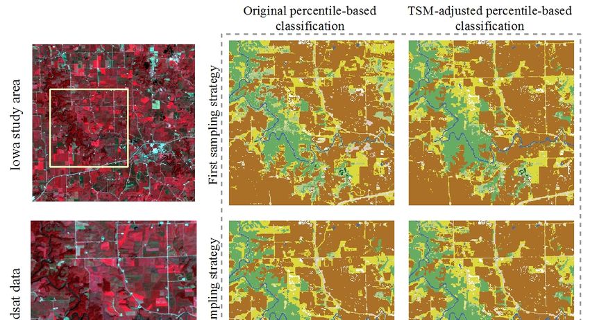
(Pixels)
                 Change Detection           Classification
                                                                                    92.6687°W to   47.4744°N to
 Minnesota               306                     12            489 × 505   222.25
                                                                                     92.4689°W      47.6056°N
                                                                                    91.1540°W to   42.2589°N to
   Iowa                  318                     14            545 × 562   275.66
                                                                                     90.9542°W      42.4026°N
Remote Sens. 2020, 12, 3091                                                         76.0972°W to   41.9614°N to 24
                                                                                                           6 of
 New York                 299                    13            541 × 558   271.69
                                                                                     75.8974°W      42.1057°N

3.3.Methodology
    Methodology
     The
      The proposed
           proposedTSM-adjusted
                       TSM-adjustedpercentile
                                        percentilemethod
                                                    methodconsisted  of of
                                                             consisted  twotwo
                                                                             major  steps
                                                                                 major     (Figure
                                                                                        steps       2): (1)
                                                                                               (Figure   2):
development    of the
 (1) development    oftime-series models
                        the time-series    and continuous
                                         models             changechange
                                                  and continuous    detection, and (2) and
                                                                            detection, percentile  feature
                                                                                            (2) percentile
generation.  In this study,
 feature generation.  In thisthe TSM-adjusted
                              study,            percentile
                                     the TSM-adjusted      featuresfeatures
                                                        percentile   were then
                                                                            wereutilized to classify
                                                                                  then utilized       land
                                                                                                to classify
cover.
 land cover.

                                                Flowchartofofthe
                                     Figure2.2.Flowchart
                                    Figure                    theproposed
                                                                  proposedmethod.
                                                                          method.

 3.1. Development of the Time-Series Model and Continuous Change Detection (CCD)
3.1. Development of the Time-Series Model and Continuous Change Detection (CCD)
      Clouds, cloud shadows, and ephemeral snow limit the availability of Earth observations acquired
      Clouds, cloud shadows, and ephemeral snow limit the availability of Earth observations
 by the Landsat series of satellites. Therefore, the number of clear observations (not contaminated by
acquired by the Landsat series of satellites. Therefore, the number of clear observations (not
 clouds, cloud shadows, and ephemeral snow) across a certain time span varies from pixel to pixel.
contaminated by clouds, cloud shadows, and ephemeral snow) across a certain time span varies from
 For every pixel, Fmask [27,32] and Tmask algorithms [33] were first used to mask out the clouds, cloud
pixel to pixel. For every pixel, Fmask [27,32] and Tmask algorithms [33] were first used to mask out
 shadows, and ephemeral snow to obtain the time-series of clear observations. The surface reflectance of
the clouds, cloud shadows, and ephemeral snow to obtain the time-series of clear observations. The
 different spectral bands were then estimated using three different time-series models—simple, advanced,
surface reflectance of different spectral bands were then estimated using three different time-series
 and full (Equations (1)–(3))—that included harmonic and trend components for the observations [21].
models—simple, advanced, and full (Equations (1)–(3))—that included harmonic and trend
 Which model was used depended upon the number of clear observations: 12 to 18 clear observations
components for the observations [21]. Which model was used depended upon the number of clear
 were required for the simple model; the advanced model needed 18 to 24 clear observations; the full
observations: 12 to 18 clear observations were required for the simple model; the advanced model
 model would be selected if there were more than 24 clear observations. Our ability to model the
 intra-year variation of Landsat time-series observations was improved with a more complex model.
 The least absolute shrinkage and selection operator (LASSO) regression technique was used for
 estimating the coefficients of time-series models [34,35]. The LASSO technique can minimize the
 sum of the squares of the residuals and has a constraint on the sum of the absolute values of the
 coefficients [36]. This allowed a time-series model that did not have the problem of overfitting to be
 developed [21].
                                                             2π               2π

                           ρ̂(i, x)simple = a0,i + a1,i cos     x + b1,i sin     x + c1,i x          (1)
                                                              T                T
where
x—Julian day
Remote Sens. 2020, 12, 3091                                                                                               7 of 24

i—Landsat band i (i = 1, 2, 3, 4, 5, and 7)
T—number of days of the year (T = 365)
a0,i —constant term that represents the mean for Landsat band i
a1,i , b1,i —coefficients of intra-year variation components for Landsat band i
c1,i —coefficient of inter-year variation component (slope) for Landsat band i
ρ̂(i, x)simple —surface reflectance of Landsat band i on Julian day x obtained using the simple model.

                                                                            4π               4π

                              ρ̂(i, x)advanced = ρ̂(i, x)simple + a2,i cos     x + b2,i sin     x                             (2)
                                                                             T                T
where

a2,i , b2,i —coefficients of the intra-year bimodal variation components for Landsat band i
ρ̂(i, x)advanced —surface reflectance of Landsat band i on Julian day x obtained using the advanced model.

                                                                            6π               6π

                              ρ̂(i, x) f ull = ρ̂(i, x)advanced + a3,i cos     x + b3,i sin     x                             (3)
                                                                             T                T
where

a3,i , b3,i —coefficients of intra-year trimodal variation components for Landsat band i
ρ̂(i, x) f ull —surface reflectance of Landsat band i on Julian day x obtained using the full model.

      Abrupt surface changes were detected based on comparisons of model-predicted values with real
observation data from Landsat. If the difference was larger than a given threshold on six consecutive
occasions, the pixel was identified as a changed pixel. To detect various surface change accurately,
a change was defined using all the spectral bands except for blue and TIR bands, because these
two spectral bands are quite sensitive to atmospheric effect and less sensitive to most of the surface
changes; and the change threshold was determined using root mean square error (RMSE) from the
time series model fit for each spectral band. If an abrupt surface change had occurred, a break would
occur in the time-series model and newly collected clear observations were added to fit to a new
time-series model. Figure 3 illustrates changed and stable pixels detected by the CCD. In this paper,
changed pixels were removed from further classification analyses, and labeled as “disturbed” in the
final classification
Remote Sens. 2020, 12, x maps. The
                         FOR PEER  time-series of stable pixels were used to generate the percentile features.
                                  REVIEW                                                                7 of 25

     Figure 3.
     Figure      Illustration of
              3. Illustration   of changed
                                   changed and
                                             and stable
                                                   stable pixels
                                                           pixels detected
                                                                  detected by
                                                                            by CCD.
                                                                               CCD. TheThe time-series
                                                                                           time-series models
                                                                                                         models shown
                                                                                                                   shown
     are based    on Landsat    band   4 data. The   left-hand  panel illustrates the  signal for a changed
     are based on Landsat band 4 data. The left-hand panel illustrates the signal for a changed pixel, and     pixel, and
     the vertical
     the vertical black
                    black dotted
                            dotted line
                                    line represents
                                         represents the
                                                      the change
                                                           change that
                                                                   that occurred
                                                                        occurred inin 2011.
                                                                                      2011. This
                                                                                             This pixel
                                                                                                  pixel was
                                                                                                         was labeled
                                                                                                               labeled as
                                                                                                                        as
     “disturbed”    in  the land-cover   map  for 2011.   The right-hand  panel illustrates the signal
     “disturbed” in the land-cover map for 2011. The right-hand panel illustrates the signal of a stableof a stable  pixel;
     the percentile
     pixel;            features
            the percentile       for this
                              features forland-cover   type were
                                           this land-cover         derived
                                                             type were      from from
                                                                        derived   time-series  data data
                                                                                        time-series  such such
                                                                                                           as these.
                                                                                                                 as these.

3.2. TSM-Adjusted Percentile Features

3.2.1. Method Used for Calculating Percentiles
     A temporal metric is the feasible conversion of time-series data over a given interval. Metrics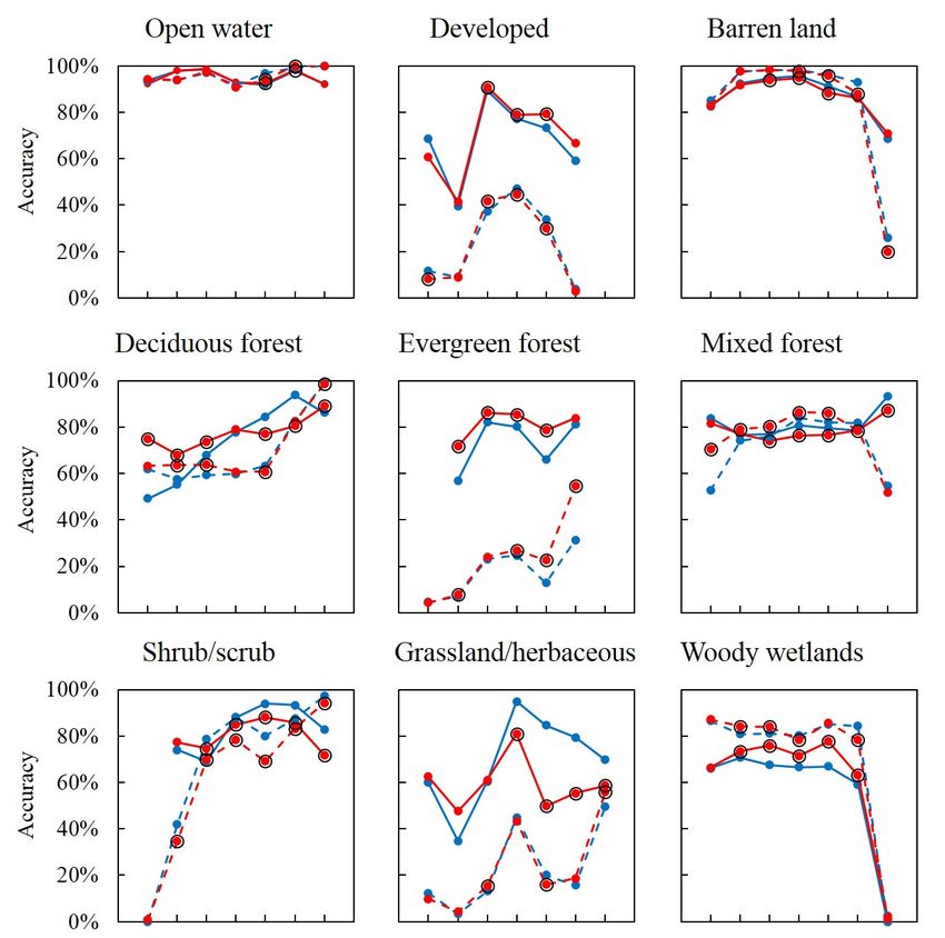
Remote Sens. 2020, 12, 3091 8 of 24
3.2. TSM-Adjusted Percentile Features
3.2.1. Method Used for Calculating Percentiles
A temporal metric is the feasible conversion of time-series data over a given interval. Metrics
can summarize the multi-temporal feature space, which captures the prominent phenological features
regardless of the specified period of year [37]. Percentiles have been commonly used as the temporal
metric in land-cover classification. Method for calculating percentiles used in this study can be
formulated as follows (Equation (4)).
ρi,ascending (R) + ρi,ascending (R + 1) /2, R ∈ N+
Pi,k = (4)
ρi,ascending (dRe), R < N+
where i denotes the ith Landsat band (i = 1, 2, 3, 4, 5, and 7); k is any number between zero and one
hundred; Pi,k denotes the kth percentile for the surface reflectance of the ith Landsat band over a given
temporal interval; ρi,ascending denotes the surface reflectance data in ascending order for the ith Landsat
band over the given temporal interval; and R is the rank of the kth percentile, which is computed as
k
R= ×N (5)
100
where N indicates the total number of clear observations for a given temporal interval. Specifically,
if the rank obtained using Equation (5) is a whole number, the kth percentile is the average of the
Rth and (R+1)th values in the surface reflectance data in ascending order; if the rank obtained using
Equation (5) is not a whole number, it is rounded up to the nearest whole number and the kth percentile
is then the dReth value in the surface reflectance data in ascending order.
3.2.2. Generation of TSM-Adjusted Percentile Features
Generally, percentile features are generated based on clear observations acquired during a given
temporal interval [13]. However, the gaps caused by clouds, cloud shadows, snow, and the SLC-off issue
lead to changes in the frequency of Landsat observations with time. According to Equations (4) and (5),
the values of percentiles are affected by the total number of clear observations and the surface reflectance
values over the given time interval. Therefore, the original percentiles features may vary for pixels
belonging to the same land-cover type but for which there are different numbers of clear observations
within the time interval. In this study, we proposed the TSM-adjusted percentile features with the
aim of characterizing land cover accurately and improving the classification accuracy substantially.
The time-series of surface reflectances were first estimated using the models based on clear observations
(detailed in Section 3.1). Next, percentile features based on synthetic time-series observations were
generated. For illustration purposes, we generated the 10th, 25th, 50th, 75th, and 90th percentile
features of a deciduous forest pixel over the period of a year based on both the original and synthetic
time-series of surface reflectances. The original percentiles were generated based on time-series of
clear observations that were temporally discrete due to the gaps resulting from the SLC-off issue and
cloud cover (see Figure 4B). The TSM-adjusted percentiles were generated based on time-series of
synthetic observations that were temporally continuous because the gaps had been estimated by the
time-series models (see Figure 4C). Therefore, the proposed TSM-adjusted percentiles completed the
total number of clear observations over a given time interval for the entire study area.
based on time-series of clear observations that were temporally discrete due to the gaps resulting
from the SLC-off issue and cloud cover (see Figure 4B). The TSM-adjusted percentiles were generated
based on time-series of synthetic observations that were temporally continuous because the gaps had
been estimated by the time-series models (see Figure 4C). Therefore, the proposed TSM-adjusted
percentiles   completed
Remote Sens. 2020, 12, 3091 the total number of clear observations over a given time interval for the entire
                                                                                                       9 of 24
study area.

     Figure 4.
     Figure        Illustrationofofthethe
              4. Illustration             generation
                                        generation  of of time-series
                                                       time-series    model
                                                                    model      (TSM)-adjusted
                                                                           (TSM)-adjusted        percentile
                                                                                             percentile     features
                                                                                                        features for
     deciduous forest: (A) time-series model based on clear Landsat band 4 observations over a given year,a
     for  deciduous     forest:  (A)   time-series  model   based  on clear Landsat    band  4 observations   over
     given
     (B) the year,
             original(B)percentile
                         the original    percentile
                                    features        features
                                             generated   usinggenerated
                                                               time-seriesusing  time-series
                                                                           of clear           of clear
                                                                                    observations,  and observations,
                                                                                                       (C) the TSM-
     and  (C) the   TSM-adjusted     percentile features  generated  using synthetic
     adjusted percentile features generated using synthetic time-series observations. time-series observations.

3.3. Classification Experiment Methodology
3.3. Classification Experiment Methodology
       The pixels that were stable over the chosen temporal interval were classified with supervised
       The pixels that were stable over the chosen temporal interval were classified with supervised
random forest (RF) classifier and the changed pixels detected by CCD were labelled as “disturbed” in
random forest (RF) classifier and the changed pixels detected by CCD were labelled as “disturbed”
land-cover maps. The percentile features, including the 10th, 25th, 50th, 75th, and 90th percentiles for
in land-cover maps. The percentile features, including the 10th, 25th, 50th, 75th, and 90th percentiles
Landsat bands 1-5 and band 7, and the NDVI (i.e., 35 features in total), were used as input data for
for Landsat bands 1‒5 and band 7, and the NDVI (i.e., 35 features in total), were used as input data
the RF classifier. The RF classifier was an ensemble machine-learning algorithm which operates by
for the RF classifier. The RF classifier was an ensemble machine-learning algorithm which operates
constructing sets of decision trees for classification during the training [38]. All the generated decision
by constructing sets of decision trees for classification during the training [38]. All the generated
trees were used to classify the newly unlabeled data, and the category receiving the largest number of
decision trees were used to classify the newly unlabeled data, and the category receiving the largest
votes will be given to this data. The forest trees were generated by setting two parameters: in this study,
number of votes will be given to this data. The forest trees were generated by setting two parameters:
we set the number of trees to 500; in addition, the number of split variables was set to the defaults,
in this study, we set the number of trees to 500; in addition, the number of split variables was set to
i.e., square root of the total number of input features. We chose RF classifier for use due to its superiority
the defaults, i.e., square root of the total number of input features. We chose RF classifier for use due
in handling high-dimensional input features without dimension reduction, its robustness against
to its superiority in handling high-dimensional input features without dimension reduction, its
outliers, as well as the high classification accuracies achieved by the use of ensemble techniques [39].
robustness against outliers, as well as the high classification accuracies achieved by the use of
       The training and testing data for the classification were collected using 2011 NLCD land cover
ensemble techniques [39].
maps of the three study areas. The four land-cover types related to impervious surfaces were spatially
       The training and testing data for the classification were collected using 2011 NLCD land cover
merged into one type named “developed”. Spatio-temporal filtering methods were used to assist in
maps of the three study areas. The four land-cover types related to impervious surfaces were spatially
the selection of highly accurate class labels. The pixels in the 2011 NLCD data were selected only if the
merged into one type named “developed”. Spatio-temporal filtering methods were used to assist in
following filtering criteria were met. First, the NLCD pixel values for 2001, 2006, and 2011 had to be
the selection of highly accurate class labels. The pixels in the 2011 NLCD data were selected only if
identical. The use of this temporal rule helped select the NLCD pixels having the identical land-cover
the following filtering criteria were met. First, the NLCD pixel values for 2001, 2006, and 2011 had to
type between 2001 and 2011. Second, the 2011 NLCD pixel had to have the same value as the eight
be identical. The use of this temporal rule helped select the NLCD pixels having the identical land-
pixels surrounding it. This spatial rule was used to help reduce 30-m pixel edge effects which may
cover type between 2001 and 2011. Second, the 2011 NLCD pixel had to have the same value as the
produce apparent mix in land cover. The generated class labels used for training and testing were
illustrated in Supplementary Materials Figure S1.
       The sampling technique adopted in this study is stratified random sampling; that is, each land
cover type is sampled independently and randomly. The number of samples collected for each type is
proportional to the area occupied by each type. Additionally, the effect of training-data balance was
also considered because an imbalanced sample size among classes would substantially decrease the
accuracies of rare class because of the very few extracted training samples [40]. A total of 3437, 1869,
and 2261 training pixels (see Table 2 for the number of training pixels of each land cover type) were
selected for the Minnesota, Iowa, and New York study areas, respectively; the remaining candidate
NLCD pixels are treated as testing data.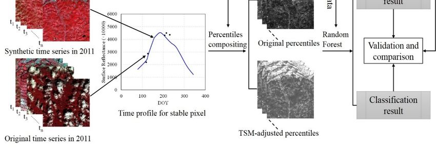
Remote Sens. 2020, 12, 3091                                                                              10 of 24

             Table 2. The number of training pixels for each land cover type in the three study areas.

                        Land Covers              Minnesota             Iowa             New York
                   Open water (OW)                   420                210                210
                     Developed (D)                   245                140                280
                    Barren land (BL)                 700                  -                 -
                 Deciduous forest (DF)               350                350                630
                  Evergreen forest (EF)              182                49                 140
                   Mixed forest (MF)                 490                140                420
                     Shrub/scrub (S)                 280                  -                 -
                Grassland/herbaceous (G)             140                 70                 -
                     Pasture/hay (P)                   -                350                420
                 Cultivated crops (CC)                 -                560                 -
                 Woody wetlands (WW)                 560                  -                161
               Herbaceous wetlands (HW)               70                  -                 -

      The NLCD class labels and the original and proposed TSM-adjusted percentile features were
extracted for each training sample. The original percentiles were also extracted in order to compare
the classification results obtained using the proposed TSM-adjusted percentiles with those obtained
using the original percentiles. The RF classification results were generated using the training data;
these results were then quantitatively assessed using the common classification accuracy metrics of
overall accuracy (OA), per-class producer’s accuracy (PA) and user’s accuracy (UA), which were
derived from the confusion matrices using the corresponding test data [41]. To apply the statistical
significance testing, the above classification experiment was conducted repeatedly 10 times. Paired
t-tests were used to determine if the differences in accuracy of the two sets of classifications were
significant at the 5% level. In addition, a final land cover classification was generated for the spatial
visualization using the most frequent category from the 10 individual ones.
      In order to investigate the effect of valid observation frequency and training data sampling strategy
on classification results, some other experiments were performed, and the results were presented in
Sections 5.2 and 5.3. In Section 5.2, the classification accuracies of land cover types with different
numbers of valid observations were calculated. More specifically, for each independent classification
experiment, the test data for each land-cover type were stratified according to valid observation counts,
and then the accuracy for each layer was calculated by comparing the classified data against the
corresponding test data. More specifically in Section 5.3, in addition to the sampling strategy used in
previous experiments, i.e., random sampling across valid observation frequency stratums for each
class, another two sampling strategies were used, i.e., random sampling from the pixels with low (high)
observation frequencies for each class. The experiments were designed to test the robustness of the
proposed TSM-adjusted percentiles to the sampling strategies of training data.

4. Results

4.1. Classification of Percentiles Derived from Multispectral Reflectance and NDVI Time Series
     The original and TSM-adjusted percentiles that were respectively derived from the original and
synthetic Landsat 6-bands reflectances and NDVI time-series for April to October of the climatological
year 2011 were classified. A comparison of the classification results obtained using the original
percentiles with those obtained using the proposed TSM-adjusted percentiles provided insights
into whether using the TSM-adjusted percentiles led to improved classification results. The overall
accuracies of original and TSM-adjusted percentiles-based classification results are summarized in
Table 3. The overall accuracies derived from the TSM-adjusted percentiles are significantly higher than
those derived from the original percentiles in any single selected test area. This indicates that compared
to original percentiles, the proposed TSM-adjusted percentiles have the improved overall classification
performance. In addition, the standard deviations in the OA for the TSM-adjusted percentiles-based
Remote Sens. 2020, 12, 3091 11 of 24
classification are smaller than those for the original percentiles-based classification for all three study
areas. This result suggests that the former yielded more stable results than the latter. The original
percentiles for training and test pixels randomly selected each time might exhibit some degree of
variability in the repeatedly performed experiments, because the uneven temporal distribution of
valid observations exist in the original time series from which the original percentiles were derived.
In contrast, the TSM-adjusted percentiles are produced from the synthetic time-series observations
without gaps resulting from clouds, cloud shadows, snow, and missing data. Thus, the uncertainty in
the temporal distribution of observations for training and test data can be alleviated.
Table 3. Overall classification accuracies achieved by the use of original percentiles and TSM-adjusted
percentiles for the three study areas. The average values and standard deviations (in parentheses)
of the overall accuracies were derived from ten independent classification experiments. Note that the
upward arrows indicate that the overall accuracies obtained using the TSM-adjusted percentiles are
significantly (at the 5% level) higher than that obtained using the original percentiles.
Study Area Original Percentiles-Based Classification TSM-Adjusted Percentiles-Based Classification
Minnesota 81.98% (0.35%) 82.82%↑(0.33%)
Iowa 93.53% (0.63%) 94.31%↑(0.38%)
New York 85.99% (0.41%) 90.05%↑(0.39%)
Table 4 summarizes the user’s and producer’s accuracies of each land cover class for original
percentiles-based classification, and the counterpart for TSM-adjusted percentiles-based classification
are given in Table 5. User’s accuracy of one land cover class is the ratio of the number of pixels
correctly classified as that class to the total number of pixels classified as that class; the relative higher
user’s accuracy indicates fewer commission errors. Producer’s accuracy of one land cover class is the
ratio of the number of pixels correctly classified as that class to the total number of pixels specified
as that class in the reference data; the relative higher producer’s accuracy indicates fewer omission
errors. The significant difference of UA and PA between the two sets of classification was reported
in Table 5. This result indicated that the improvements obtained using the proposed method were
different between specific land cover classes, and also between producer’s and user’s accuracies for
the same class. Further, these results also varied across the three study areas. In order to discuss the
difference in improvements obtained from the proposed method between specific land cover classes
and across the three study areas, we chose five different land cover types (i.e., open water, developed,
deciduous forest, evergreen forest, and mixed forest) as examples for analysis in Sections 4.1, 5.1 and 5.2
because they can be found in all three study areas.
Table 4. Average producer and user accuracies of the classifications derived from original percentiles
(see Table 3 for the associated overall accuracies). Ten independent classification experiments in total
were carried out.
OW D BL DF EF MF S G WW HW
Minnesota UA 95.13% 32.51% 96.78% 63.89% 17.72% 78.26% 83.71% 23.95% 81.86% 51.84%
PA 95.86% 77.42% 93.03% 72.18% 75.32% 78.74% 89.31% 83.28% 67.53% 62.89%
OW D DF EF MF G P CC
Iowa UA 64.09% 9.90% 96.08% 84.43% 5.05% 4.56% 55.10% 99.33%
PA 90.58% 71.41% 90.75% 90.00% 73.33% 37.66% 86.02% 94.35%
OW D DF EF MF P WW
New York UA 99.24% 67.36% 94.46% 19.29% 70.29% 84.43% 20.43%
PA 99.53% 74.27% 87.60% 61.28% 75.30% 92.46% 57.56%Remote Sens. 2020, 12, 3091 12 of 24
Table 5. Average producer and user accuracies of the classifications derived from TSM-adjusted
percentiles (see Table 3 for the associated overall accuracies). Ten independent classification experiments
in total were carried out. Note that the upward (downward) arrows indicate that the accuracies obtained
using the TSM-adjusted percentiles are significantly (at the 5% level) higher (lower) than that obtained
using the original percentiles. Figure without arrow behind it represents that there is no significant
difference between the two sets of classification.
OW D BL DF EF MF S G WW HW
Minnesota UA 94.96% 31.57% 96.12%↓ 65.84%↑ 21.14%↑ 82.25%↑ 74.90%↓ 23.20% 83.02%↑ 32.17%↓
PA 95.73% 79.80%↑ 91.84%↓ 75.60%↑ 82.71%↑ 76.16%↓ 84.36%↓ 66.94%↓ 73.67%↑ 52.47%↓
OW D DF EF MF G P CC
Iowa UA 60.70%↓ 9.57% 96.54% 83.84% 5.37% 3.24%↓ 60.79%↑ 99.29%
PA 90.53% 64.93%↓ 91.37%↑ 91.33% 80.00%↑ 43.13%↑ 84.53%↓ 95.31%↑
OW D DF EF MF P WW
New York UA 99.17% 64.87%↓ 97.07%↑ 26.58%↑ 83.64%↑ 88.05%↑ 17.88%↓
PA 98.97%↓ 81.90%↑ 91.77%↑ 79.01%↑ 83.12%↑ 91.73%↓ 75.75%↑
More specifically, the accuracies of open water had no significant difference, but it had lower UA in
Iowa and lower PA in New York. The improvement of developed was seen in terms of PA in Minnesota
and New York, but its PA was lower in Iowa and its UA was lower in New York. The accuracies
of deciduous forest were significantly improved across all three study areas except the UA in Iowa.
Evergreen forest had higher UA and PA in Minnesota and New York but had no significant difference
in classification accuracy in Iowa. The PA of Mixed forest was improved in Iowa and New York but
was decreased in Minnesota; the UA of it was improved in Minnesota and New York, but have no
significant difference in Iowa.
4.2. Spatially Explicit Classification Results
This section provides a spatial visualization of the classification results obtained using the original
and TSM-adjusted percentiles (see Figure 5). An individual final classification result of any single test
area is produced instead of examining the 10 random independent classification results (see Tables 3–5
for a summary of the associated classification accuracy metrics). The final classification results were
obtained by assigning the most frequent category in the 10 random forest classifications to each pixel.
The land-cover changes detected by the CCD algorithm for 2011 were labeled as “disturbed” in the
final classification results.Remote Sens. 2020, 12, 3091 13 of 24
Remote Sens. 2020, 12, x FOR PEER REVIEW 14 of 25
Figure
Figure 5. 5. Spatiallyexplicit
Spatially explicitclassifications
classifications of
of the
the three study
study areas
areasfor
forthe
thetarget
targetyear
year2011.
2011.Left-hand
Left-hand
column: the final classifications generated using 10 independent random
column: the final classifications generated using 10 independent random forest (RF) supervised forest (RF) supervised
classification
classification resultsofoforiginal
results originalpercentiles.
percentiles. Right-hand
Right-hand column:
column: thethefinal
finalclassifications
classificationsgenerated
generated
using 10 independent RF supervised classification results of proposed
using 10 independent RF supervised classification results of proposed TSM-adjusted TSM-adjusted percentiles. Top:
percentiles.
Minnesota
Top: Minnesota classification
classificationresults, middle:
results, middle: IowaIowaclassification
classificationresults, andand
results, bottom:
bottom:NewNew York
York
classification
classification results.Colors
results. Colorscorrespond
correspond to to those
those used
used in inFigure
Figure11except
exceptforforthe
the“Developed”
“Developed” class,
class,
which
which is rendered
is rendered inin lightpink.
light pink.White
Whiteshows
shows the the pixel
pixel locations
locationswhere
whereland-cover
land-cover changes
changesoccurred:
occurred:
these pixels were labeled as belonging to the “disturbed”
these pixels were labeled as belonging to the “disturbed” class. class.Remote Sens. 2020, 12, 3091 14 of 24
Remote Sens. 2020, 12, x FOR PEER REVIEW 15 of 25
5. Discussion
5.1. Effect of
5.1. Effect of Phenological
Phenological Characteristics
Characteristics
The mechanisms producing
The mechanisms producingthe thechanges
changesininsurface
surface reflectance
reflectance over
over timetime varied
varied according
according to
to the
the land-cover type. For example, the reflectance of deciduous forest changed
land-cover type. For example, the reflectance of deciduous forest changed over time due to the over time due to the
phenological
phenological characteristics. For cover
characteristics. For cover types
types that
that have
have nono seasonal
seasonal features,
features, suchsuch as as open
open water,
water,
changes in illumination
changes in illuminationgeometry
geometryled ledtotothe
thechanges
changes in in surface
surface reflectance
reflectance (due(due to, example,
to, for for example,
the
the bidirectional reflectance distribution function (BRDF) effect). Nevertheless,
bidirectional reflectance distribution function (BRDF) effect). Nevertheless, the magnitude of the the magnitude of the
changes
changes caused
caused byby the
the illumination
illumination geometry
geometry was was much
much smaller
smaller than
than that
that caused
caused by by phenological
phenological
characteristics.
characteristics. Figure
Figure6 illustrates the the
6 illustrates changes in Landsat
changes band-4band-4
in Landsat reflectance in 2011 for
reflectance in the deciduous
2011 for the
forest and open water cover types. It is evident that the band-4 reflectance reached its
deciduous forest and open water cover types. It is evident that the band-4 reflectance reached its peak peak during the
growing
during theseason for deciduous
growing season for forest
deciduousand that forand
forest open water
that it didwater
for open not vary significantly
it did during the
not vary significantly
whole year.
during the whole year.
Figure 6. Illustration of Landsat band-4 time-series for open water and deciduous forest in 2011.
Figure 6. Illustration of Landsat band-4 time-series for open water and deciduous forest in 2011.
Figure 7 illustrates the differences in PA and UA between the TSM-adjusted and original
Figure 7 illustrates the differences in PA and UA between the TSM-adjusted and original
percentiles-based classifications for the three study areas to show how the improvement in classification
percentiles-based classifications for the three study areas to show how the improvement in
accuracies using the proposed TSM-adjusted percentiles varied by cover type and across different
classification accuracies using the proposed TSM-adjusted percentiles varied by cover type and
study areas. As expected, the improvement both in UA and PA for deciduous forest, evergreen forest,
across different study areas. As expected, the improvement both in UA and PA for deciduous forest,
and mixed forest were consistently observed across all the three study areas (except for the slightly
evergreen forest, and mixed forest were consistently observed across all the three study areas (except
lower PA of mixed forest in Minnesota); the improvement was most significant in New York study
for the slightly lower PA of mixed forest in Minnesota); the improvement was most significant in
area, followed by Minnesota and least significant in Iowa. On the other hand, higher PA for forest
New York study area, followed by Minnesota and least significant in Iowa. On the other hand, higher
types with less improvement in UA would indicate lower rates of omission (more of what is forest
PA for forest types with less improvement in UA would indicate lower rates of omission (more of
in the reference data is captured as such by the adjusted percentile feature classification), but similar
what is forest in the reference data is captured as such by the adjusted percentile feature
rates of commission (the adjusted percentile feature classification still misclassifies other classes as
classification), but similar rates of commission (the adjusted percentile feature classification still
forest at the same levels). There is no noteworthy improvement in classification accuracy for open
misclassifies other classes as forest at the same levels). There is no noteworthy improvement in
water across the three study areas using the proposed method (except for the slightly lower UA of
classification accuracy for open water across the three study areas using the proposed method (except
open water in Iowa). These results can be interpreted by considering that the percentiles capture the
for the slightly lower UA of open water in Iowa). These results can be interpreted by considering that
magnitude of time-series reflectances. The gaps in time-series observations that are used to generate
the percentiles capture the magnitude of time-series reflectances. The gaps in time-series observations
percentile features have little impact on open water, where there is little change in reflectance over time.
that are used to generate percentile features have little impact on open water, where there is little
However, these gaps have a great impact in the case of deciduous, evergreen and mixed forest where
change in reflectance over time. However, these gaps have a great impact in the case of deciduous,
there are great changes in reflectance over time due to phenological characteristics; this is especially
evergreen and mixed forest where there are great changes in reflectance over time due to
true in frequently cloud-covered areas—i.e., the areas with fewer valid observations. Thus, the original
phenological characteristics; this is especially true in frequently cloud-covered areas—i.e., the areas
percentiles derived from pixels with fewer valid observations might be not as much reliable to produce
with fewer valid observations. Thus, the original percentiles derived from pixels with fewer valid
accurate classification results as that derived from pixels with a good number of valid observations.
observations might be not as much reliable to produce accurate classification results as that derived
In contrast, the proposed TSM-adjusted percentiles could normalize the number of valid observations
from pixels with a good number of valid observations. In contrast, the proposed TSM-adjusted
for pixels using time series models. As a result, compared to using original percentiles, the use of
percentiles could normalize the number of valid observations for pixels using time series models. As
TSM-adjusted percentiles can significantly improve the classification accuracy for forest with obvious
a result, compared to using original percentiles, the use of TSM-adjusted percentiles can significantly
phenological characteristics. The developed class exhibited a certain degree of uncertainty in accuracy
improve the classification accuracy for forest with obvious phenological characteristics. The
developed class exhibited a certain degree of uncertainty in accuracy variation across the three study
areas, due to the complex spectral heterogeneity of the developed type. For example, the developedRemote Sens. 2020, 12, 3091 15 of 24
variation
Remote Sens.across the
2020, 12, three
x FOR study
PEER areas, due to the complex spectral heterogeneity of the developed16type.
REVIEW of 25
For example, the developed type in NLCD consists of four sub-types with different levels of mixture of
type in NLCD
constructed consistsand
materials of four sub-types
vegetation. with different
Therefore, levelsand
the seasonal of mixture of constructed
non-seasonal materialsboth
spectral variation and
vegetation.
exist Therefore,
in developed type.the seasonal and non-seasonal spectral variation both exist in developed type.
Figure
Figure 7. The differences
7. The differences in
in PA
PA and
and UA
UA between
between the
the TSM-adjusted
TSM-adjusted and
and original
original percentiles-based
percentiles-based
classification
classification for individual land-cover types in Minnesota (a), Iowa (b), and New York(c).
for individual land-cover types in Minnesota (a), Iowa (b), and New York (c).
5.2. Effect of the Frequency of Valid Observations
5.2. Effect of the Frequency of Valid Observations
Missing data resulting from clouds, cloud shadows, snow, and the SLC-off problem is normal in
Missing data resulting from clouds, cloud shadows, snow, and the SLC-off problem is normal
Landsat observation time-series. Although the implementation of percentile compositing can alleviate
in Landsat observation time-series. Although the implementation of percentile compositing can
the impact of missing data, the more missing data there are, the less reliable the resulting percentile
alleviate the impact of missing data, the more missing data there are, the less reliable the resulting
bands. Generally the distribution of missing satellite observations is not even over time [42–44]
percentile bands. Generally the distribution of missing satellite observations is not even over time
and, consequently, the number and acquisition date of valid observations varied by pixels. Figure 8
[42–44] and, consequently, the number and acquisition date of valid observations varied by pixels.
illustrates the spatial patterns in the frequency of valid observations for the three study areas in 2011.
Figure 8 illustrates the spatial patterns in the frequency of valid observations for the three study areas
The corresponding histograms of the valid observations frequency for each study area were shown in
in 2011. The corresponding histograms of the valid observations frequency for each study area were
shown in Figure S2. In addition, the level of time series models (simple, advanced, and full) used for
surface reflectance estimation in 2011 for each pixel of each study area were provided in Figure S3.Remote Sens. 2020, 12, 3091 16 of 24
FigureSens.
Remote S2.2020,
In addition, the level
12, x FOR PEER of time
REVIEW series models (simple, advanced, and full) used for surface
17 of 25
reflectance estimation in 2011 for
Remote Sens. 2020, 12, x FOR PEER REVIEW each pixel of each study area were provided in Figure S3. 17 of 25
Figure 8. Spatial patterns in the number of valid observations in 2011 for the three study areas. (left):
Minnesota; (middle):
Spatial
Figure8.8.Spatial
Figure Iowa;
patterns
patterns and
in the (right):
in the number
number New
of ofYork.
valid
valid observations
observations in for
in 2011 2011thefor thestudy
three three areas.
study(left):
areas.
(left): Minnesota; (middle): Iowa; and (right):
Minnesota; (middle): Iowa; and (right): New York. New York.
As can clearly be seen from Figure 9, the profiles of the original reflectance time-series of
As can clearlysamples
deciduous be seen from Figure 9, the profilesof ofvalid
the original reflectance time-series of deciduous
As canforest
clearly be seen with
fromdifferent
Figurenumbers
9, the profiles ofobservations
the originalare different;time-series
reflectance however, the
of
forest
profilessamples
of the with different
synthetic numbers
reflectance of valid
time-series observations
estimated by are
the different;
time-series however,
models the
are profiles
similar of the
for all
deciduous forest samples with different numbers of valid observations are different; however, the
synthetic
of the reflectance
deciduous time-series
forest samples estimated
regardless byofthe time-series
valid models
observation are similar
counts. In for
fact, allpercentile
the of the deciduous
values
profiles of the synthetic reflectance time-series estimated by the time-series models are similar for all
forestaffected
were samplesby regardless
the number of valid observation
andregardless
magnitude counts. In fact, the percentile values were affected by
of the deciduous forest samples of of the observation
valid time-series data,
counts.according
In fact, tothethe formulae
percentile given
values
theSection
in number andTherefore,
3.2.1. magnitude it of
wastheexpected
time-series
that data, accordingTSM-adjusted
the time-series
proposed to the formulae given inderived
percentiles Section from
3.2.1.
were affected by the number and magnitude of the data, according to the formulae given
Therefore,
the synthetic it was expected
time-series thatless
were theinfluenced
proposed TSM-adjusted
by valid percentiles
observation derived
frequency, andfrom
thatthe synthetic
they would
in Section 3.2.1. Therefore, it was expected that the proposed TSM-adjusted percentiles derived from
time-series
show less were less influenced
variation and by valid
be less
more observation
accurate than frequency,
those and that using
obtained they would
originalshowtime-series
less variation
in
the synthetic time-series were influenced by valid observation frequency, and that they would
and be more accurate
characterizing than those obtained using original time-series in characterizing land-cover.
land-cover.
show less variation and be more accurate than those obtained using original time-series in
characterizing land-cover.
Figure 9.
Figure 9. Illustration
Illustrationofof
Landsat band-4
Landsat time-series
band-4 of deciduous
time-series forest samples
of deciduous with different
forest samples numbers
with different
of valid
numbers observations during the year 2011. (The black dots indicate original time-series observations
Figure 9. of valid observations
Illustration of Landsat during
band-4thetime-series
year 2011. of
(The black dots
deciduous indicate
forest original
samples withtime-series
different
and blue curves
observations andindicate
blue synthetic
curves time-series).
indicate synthetic time-series).
numbers of valid observations during the year 2011. (The black dots indicate original time-series
observations
The effect ofand blue
valid curves indicate
observation synthetic
frequency time-series).
(i.e., the number of valid observations) was examined by
The effect of valid observation frequency (i.e., the number of valid observations) was examined
calculating the classification accuracies of land cover types with different numbers of valid observations.
by calculating
The10–12 the classification
effect illustrate
of valid observation accuracies
frequency of(i.e.,
landthecover
number types withobservations)
of valid different numbers
was of valid
examined
Figures the responses of the classification accuracies for each land cover class to valid
observations.
by calculating Figures 10–12
the classificationillustrate the
accuracies responses of
of evident,
land coverthe classification
typeswater accuracies
with and different for each
numbers land cover
observation counts in the three study areas. As for open developed types,ofthere
validis
class to valid
observations. observation
Figures 10–12 counts in
illustrate the three
the responsesstudy areas.
of the As evident,
classification for open water and
accuraciespercentiles developed
for each land
no obvious difference between the accuracies obtained using the TSM-adjusted andcoverthose
types,
class to there
valid is no obvious
observation countsdifference between
in the regardless
three studythe accuracies obtained using theand
TSM-adjusted
obtained using the original percentiles ofareas. As evident,
the number for observations,
of valid open water developed
except for UA
percentiles
types, there and
is nothose obtained
obvious using
difference the original
between the percentiles
accuracies regardless
obtained of
usingthe number
the of valid
TSM-adjusted
curve of open water in Iowa and PA curve of developed in New York. By contrast, for deciduous
observations,
percentiles except for UA curve of open water in percentiles
Iowa and PA curve of developed in New York.
forest in alland
threethose
studyobtained
areas and using the original
evergreen forest in Minnesotaregardlessand New of thestudy
York number
areas,of the
valid
PA
By contrast,
observations, for deciduous
except for UA forest
curve in all
of three
open study
water inareas
Iowa and
and evergreen
PA curve forest
of in Minnesota
developed in Newand New
York.
obtained by using the TSM-adjusted percentiles are much better than those obtained using the original
York
By study areas,
contrast, the PA obtained
for deciduous in by
all using the TSM-adjusted percentiles are in much better than
and those
percentiles especially whenforest
the number three study
of valid areas and evergreen
observations is lower; forest Minnesota
the PA difference between New
the
obtained
York study using
areas, thetheoriginal
PA percentiles
obtained by usingespecially
the when
TSM-adjusted the number
percentilesof valid
are observations
much better thanis lower;
those
two sets of results becomes smaller as the number of valid observations increases. Interestingly, except
the PA difference
obtained using thebetween
originalthe two sets of
percentiles results becomes
especially when the smaller
number as the
of number of valid observations
valid observations is lower;
increases. Interestingly, except for evergreen forest in Iowa
the PA difference between the two sets of results becomes smaller as the number of and mixed forest in Minnesota and New
valid observations
York study
increases. areas, UA curves
Interestingly, exceptfor forforest types forest
evergreen showed in no
Iowaobvious
and mixeddifference
forestininperformance
Minnesota and between
New
original percentiles-based and TSM-adjusted percentiles-based classification
York study areas, UA curves for forest types showed no obvious difference in performance between across the different
original percentiles-based and TSM-adjusted percentiles-based classification across the differentYou can also read