INTEGRATE MACHINE
LEARNING MODELS
WITH PYTHON AND
MICROSTRATEGY
←
→
Page content transcription
If your browser does not render page correctly, please read the page content below

INTEGRATE MACHINE LEARNING MODELS WITH PYTHON AND MICROSTRATEGY
Thank you for participating in a workshop at
 MicroStrategy World 2019. If you missed or did
 not finish an exercise and want to complete it
 after the conference, use this workbook and
 access the supporting files at
 microstrategy.com/world-2019-workshops

*Workshop files will expire 4/30/2019
Integrate Machine Learning Models
Integrating Python Machine Learning Models and MicroStrategy

              with Python and MicroStrategy

                    MicroStrategy offers features that enable analysts and data scientists to use
                    machine learning to extract meaningful insights from their data for a variety of use
                    cases and problems, including out-of-the-box functions and basic algorithms.
                    However, data scientists often rely on a wide range of tools, especially open-
                    source coding languages like R and Python. To support those tools, data scientists
                    can now code the language of their choice and continue to use MicroStrategy via
                    open-source packages.

                    The purpose of this session is to show you how MicroStrategy and Python can
                    work together to produce machine learning results within the context of business
                    intelligence. In this workshop, you will:

                    •   Learn what actually happens when building a machine learning model and
                        explore a framework for thinking about the model building life cycle.

                    •   Train a deep learning network to predict flight delays in Python.

 Learn why a BI system is a core piece of the technology stack that enables data science teams
 to be successful. Machine Learning 101

 Broad definition
                    Machine learning (ML) can be loosely defined as statistical and mathematical
                    techniques that allow computer systems to learn from data.

  3 Walk-through: Modeling                                                         © 2018 MicroStrategy, Inc.

4 | MicroStrategy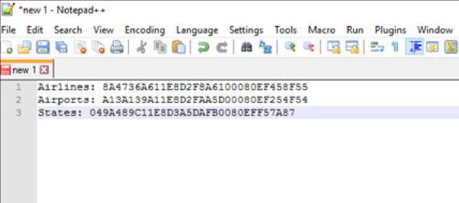
MicroStrategy World 2019 Workshop Book
Machine Learning                                                                    Machine Learning
                                                                                                         1

                Machine learning implies that the performance of a specific task is progressively
                improved. To achieve this, different algorithms can be exposed to historical data
                to create a trained model, and then tested on unseen data to evaluate how well
                the model performs.

Common examples
                Examples of ML are more common than you think. Some you may be aware of:

                •   Selecting the next song in a playlist on a streaming service.
                •   Granting or denying a loan when you apply.
                •   Curating the news feed on a social media site.
                •   Product placement ads in your browser.

Exercise 1: Training with iris data
                To get our feet wet with machine learning, let’s look at an example with a dataset
                often used to introduce data science techniques: the iris dataset. This data, shown
                below, contains the dimensions of the sepals and petals of a flower, and the
                species these sets of measurements belong to within the iris genus.

                     The dimensions of an iris can be used to learn how to classify it into the
                     species it belongs to. Let’s use an interactive site to explore and observe the
                     data points.

© 2018 MicroStrategy, Inc.                                                      Walk-through: Modeling   4
                                                                                                  MicroStrategy | 5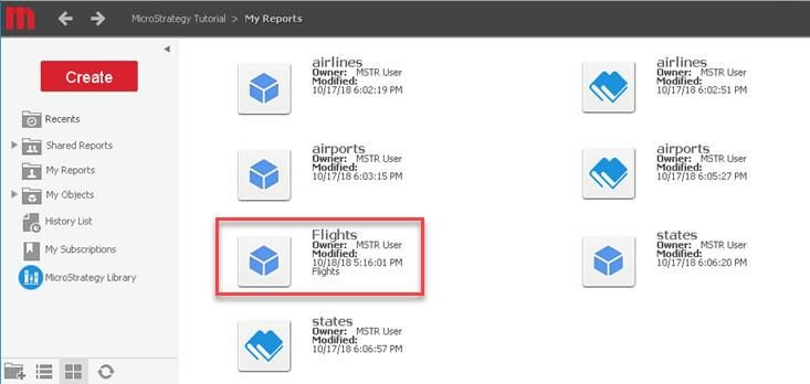
Integrating Python Machine Learning Models and MicroStrategy
        Machine Learning                                                                       Machine Learning
   1

                    1 Open a browser and navigate to:
                       https://plot.ly/~AmenRadix/128.embed
                             The page displays a graph similar to the image below. You can
                             intuitively identify three clusters.
                                                                           Exercise 1: Training with iris data

                             Without having to create any algorithms, your brain trained itself to
                             view the clusters. Our brains are good at abstracting up to three
                             dimensions when we have a visual representation of the model. But
                             what happens when you have five dimensions—or ten? It becomes
                             much harder. Now imagine a weather system where thousands of
                             factors are taken into account.

                             This is why it is important to have a framework to manage, train, and
                             evaluate models. Among those frameworks, many data scientists will
                             operate using the CRISP-DM, discussed below.

  5 Walk-through: Modeling                                                           © 2018 MicroStrategy, Inc.
6 | MicroStrategy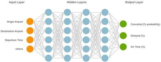
MicroStrategy World 2019 Workshop Book
Machine Learning                                                                  Machine Learning
                                                                                                       1

CRISP-DM framework
                Companies around the world use machine learning to create insights into their
                businesses. But how does one create a machine learning system?

                Many data science teams use a process framework, CRISP-DM, to guide their work.
                CRISP-DM stands for Cross-Industry Standard Process for Data Mining. It lays out
                the fundamental steps common to nearly every machine learning project. Here’s a
                diagram that visualizes the framework:

                The process is a cycle, and starts with business understanding.

Business understanding
                Business understanding is about trying to identify both the core drivers of and
                problems with your business. In this part of the process, it is vital to spend time
                examining the business problems that might be good candidates to approach with
                machine learning.

© 2018 MicroStrategy, Inc.                                                    Walk-through: Modeling   6
                                                                                                MicroStrategy | 7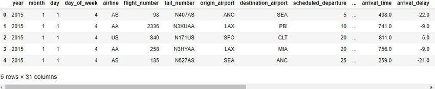
Integrating Python Machine Learning Models and MicroStrategy
        Machine Learning                                                                    Machine Learning
   1

                                                                                     CRISP-DM framework

                    You may find it helpful to imagine what it would be like to solve the business
                    problem you’re working on with machine learning. What would it mean to use
                    algorithms to help find a solution? How would they be adapted internally?

 Data understanding
                    The next step is data understanding. Once we’ve identified our problem, we need
                    to take inventory of the data that might be useful for analysis. We need to seek
                    out high quality, reliable, and reproducible sources of data. We need to also spend
                    a lot of time understanding what the data contains, and more importantly, what it
                    doesn’t contain.

                    Sometimes at this stage, you need to go back to the business understanding step
                    and re-examine the problem in light of the available data. You’ll see that this back
                    and forth behavior is common in the CRISP-DM framework and in data science
                    projects in the real world.

 Data preparation
                    Many data scientists use a rule of thumb that you should expect to spend about
                    80% of a data science project on data preparation. This includes data clean-up,
                    creating new variables, writing code to extract data from databases, and
                    reorganizing the data in a way that machine learning algorithms need it to be
                    structured.

                    This is a critical step of the project because you’re building the “plumbing” that
                    every subsequent step in the machine learning process relies on. It is not
                    uncommon to get to the modeling step of a project only to realize that something
                    critical was missed during data preparation. For this reason, many data scientists
                    build automated pipelines to manage data preparation.

 Modeling
                    In the modeling phase, we choose from among hundreds of algorithms that might
                    work for our problem. For example, in a time-series forecasting problem, you
                    might want to use a moving-average based model or something that takes
                    seasonality and time dependence into account, such as ARIMA.

  7 Walk-through: Modeling                                                          © 2018 MicroStrategy, Inc.
8 | MicroStrategy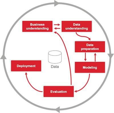
MicroStrategy World 2019 Workshop Book
Machine Learning                                                                 Machine Learning
                                                                                                       1

                It’s common to decide on a basket of modeling approaches, rather than relying on
                just one, and quantitatively evaluating which model is best.

Evaluation
                In the evaluation stage, you assess how each of the algorithms performed using an
                objective scoring approach. You may have heard of r-squared or mean squared
                error for example. These are all evaluation metrics used to help data scientists
                understand whether the algorithm has been successful in generalizing the
                problem.

                Another important part of this step is checking the quality of the model in
                business terms. This means that we revisit our business problem and ask ourselves
                if the model will be helpful in our business context.

Deployment
                Finally, we have to deploy our model! The real return on investment from
                machine learning comes from organizations successfully deploying their models
                into production and integrating them in the decision-making fabric of their
                organization.

                Now that we are familiar with the CRISP-DM framework, let’s put it in action for a
                specific problem: predicting flight delays.

© 2018 MicroStrategy, Inc.                                                    Walk-through: Modeling   8
                                                                                               MicroStrategy | 9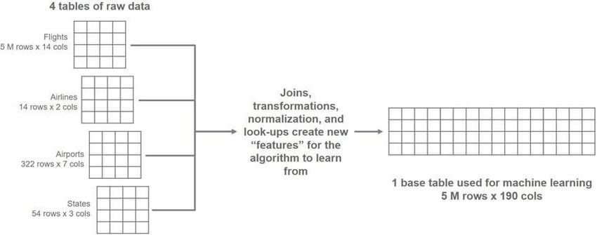
Integrating Python Machine Learning Models and MicroStrategy
         Machine Learning                                                                    Machine Learning
     1

   Walkthrough: Business understanding

                     Let’s assume we are members of the analytics team at a major US airport. We have
                     data on every inbound and outbound flight for an entire year—over 5 million flights.
                     We also have the outcome of each flight: whether it was canceled, delayed, or left
                     on-time.

                     Our primary goal is to train a model that predicts the probability that each flight
                     will be canceled, delayed, or leave on time. Our secondary goal is to use those
                     predictions to display this information to passengers, so they are proactively
                     informed about their flight’s status.

                     For this workshop, we will be using four datasets. We will also pull external region
                     data into MicroStrategy to create a new Intelligent Cube.

   9 Walk-through: Modeling                                                          © 2018 MicroStrategy, Inc.
10 | MicroStrategy
MicroStrategy World 2019 Workshop Book
Machine Learning Machine Learning
1
• Flights: This dataset contains data on over 5 million individual flights from
2015. The data contains dates and times for each flight, flight destination,
flight departure airport, the airline, and other core data.
• Airlines dataset: This dataset contains 14 airline names and their
corresponding airline code.
• Airport: This dataset contains data on 322 airports, along with their state, city,
latitude, and longitude.
• US States: This dataset contains information about each of the 50 US states
and territories.
At this step of the process, it’s good practice to start making a list of potential
features—new variables—to add that are not available in the raw data. Later in
the data prep process, we’ll add that data to the raw data using Python functions.
A good initial hypothesis is that weather—especially winter weather—has a lot to
do with flight cancellations. Another hypothesis is that there are groups of states
in regions like the northeast that experience intense winter weather, and
therefore might have a higher chance of experiencing flight delays. We will use
region codes to help our algorithm learn that some states share similar weather
patterns.
Walk-through: Data preparation
We’ll spend a fair amount of time in the data preparation stage. There are a few
sub-steps in the data prep phase.
• Getting data
• Data preparation
• Data splitting
Get data
The first step in our process is to physically get data to train our model with. Let’s
discuss how this is done when MicroStrategy is the data source for training the
model.
© 2018 MicroStrategy, Inc. Walk-through: Modeling 10
MicroStrategy | 11Integrating Python Machine Learning Models and MicroStrategy
Machine Learning Machine Learning
1
MicroStrategy solutions to these challenges
We’ll need a way to connect our machine learning server with our BI system and
extract the data. Using the MicroStrategy REST API, we’ll extract the data in our
MicroStrategy cubes and make a copy of the data locally to train our model.
We’ll use Python and a few popular machine learning packages throughout this
workshop.
We’ll use scikit-learn and its helper functions to help structure our data and
evaluate the accuracy of our final models. We will also use Keras, which is a neural
network library that interfaces with Google’s TensorFlow library, to create and
train our model.
Exercise 1: Get your own ML environment
To start, we need to connect to a MicroStrategy on AWS environment that’s
been pre-configured with the ML tools and data needed to complete the
exercises below.
Access the provisioning console
1 Navigate to the MicroStrategy on AWS provisioning console at:
https://provision.customer.cloud.microstrategy.com/
2 On the provisioning console login page, enter the credentials provided
below:
11 Walk-through: Modeling © 2018 MicroStrategy, Inc.
12 | MicroStrategyMicroStrategy World 2019 Workshop Book
Machine Learning Machine Learning
1
• Username: Cloudmicrostrategy@gmail.com
• Password: workshopmstr!
3 Find the environment with the number that your instructor provided you
with at the beginning of the workshop.
4 In the Actions section, select the ellipses icon and click Edit Contact.
5 In the Edit Contact Information window, replace the information in the
boxes with your first name, last name, and email address. Then click
Apply. You will receive an email with your environment credentials.
© 2018 MicroStrategy, Inc. Walk-through: Modeling 12
MicroStrategy | 13Integrating Python Machine Learning Models and MicroStrategy
Machine Learning Machine Learning
1
Make sure to use an email address that you can access
immediately, as you will be sent an email with your environment
credentials.
6 From the MicroStrategy on AWS email, select Access MicroStrategy
Platform . Login with your MicroStrategy Badge or enter your credentials.
7 On the landing page, scroll down and hover your cursor over
Remote Desktop Gateway, then click the Launch icon that is
displayed.
8 In the Remote Desktop Connection window, in the Username and
Password boxes, type the user name and password listed in your
Welcome to MicroStrategy on AWS email.
9 Click Login.
10 On the web page, under All Connections, click Developer Instance RDP.
13 Walk-through: Modeling © 2018 MicroStrategy, Inc.
14 | MicroStrategyMicroStrategy World 2019 Workshop Book
Machine Learning Machine Learning
1
Your remote desktop session opens. Complete the rest of this
workshop in this environment.
Exercise 2: Review datasets and start analysis
Review the datasets in MicroStrategy
1 Log into MicroStrategy Web using the credentials you received in
your MicroStrategy on AWS email.
https://env-XXXXX.trial.cloud.microstrategy.com/MicroStrategy/servlet/mstrWeb
The XXXXX above represents the environment number you received in your
Welcome to MicroStrategy on AWS email.
2 Click MicroStrategy Tutorial.
3 Select Go to MicroStrategy Web in the right corner of the screen.
4 Follow these steps to create three MicroStrategy cubes from .csv files and
retrieve their IDs. These steps must be accomplished for the three datasets
(Airlines, Airports, and States) we want to import into MicroStrategy. We
will use the Airlines as an example.
a Click Create , then Add External Data.
© 2018 MicroStrategy, Inc. Walk-through: Modeling 14
MicroStrategy | 15Integrating Python Machine Learning Models and MicroStrategy
Machine Learning Machine Learning
1
b Click File from Disk.
c Click Choose Files.
d Navigate to C:\Users\mstr\Desktop\Demo\Data\Raw, and click
airlines.csv. Click Open.
e For each of the MicroStrategy cubes (Airlines, Airports, and States), do
the following:
a Save in Shared Reports under the name airlines, airports or
states. Pay attention to the name, as casing is important. Save the
dataset name in lowercase for all three of them. A
b Review the data at the bottom of the screen.
c Close the window.
d Right-click the cube and select Properties.
e Copy the ID and click OK.
f Search for Notepad++ in the search bar. Open a Notepad++
document, paste the ID and write the name of the cube beside it.
You’ll use this information later.
Your Notepad++ document should resemble the following:
15 Walk-through: Modeling © 2018 MicroStrategy, Inc.
16 | MicroStrategyMicroStrategy World 2019 Workshop Book
Machine Learning Machine Learning
1
We will conduct our analysis via a Windows server in the environment we
previously configured, using a Jupyter Notebook to render the Python scripts in a
web browser through a distribution called Anaconda. Jupyter Notebooks are
interactive, showing code output in real time and making troubleshooting easier.
1 Click the Start menu and start typing the word Anaconda.
2 When you see Anaconda Prompt, right click it and select Run as
administrator.
3 Click Yes to accept the message that opens.
4 To ensure that we’re working in the correct directory, type cd C:\Users\mstr\ ,
and hit Enter.
5 Type jupyter notebook, then click Enter.
© 2018 MicroStrategy, Inc. Walk-through: Modeling 16
MicroStrategy | 17Integrating Python Machine Learning Models and MicroStrategy
Machine Learning Machine Learning
1
If this is your first time using a Jupyter Notebook, here is a short introduction:
• Each cell contains a snippet of Python code to run.
• To run a cell, click to select it and then either press Shift+Enter on the
keyboard or click Run in the toolbar.
• You can use the + in the toolbar to add a cell to the notebook for your own
code.
• You can use the Up and Down arrows to move a cell in the notebook.
• When a cell completes its processing, a number appears in the brackets [ ]
on the left. When it’s processing, you will see a star (*). You can also look
at the circle located at the top right of the page next to the name Python 3,
as shown below. An empty circle means it’s ready, while a full circle means
it’s busy processing.
17 Walk-through: Modeling © 2018 MicroStrategy, Inc.
18 | MicroStrategyMicroStrategy World 2019 Workshop Book
Machine Learning Machine Learning
1
• If there is output from the code in a cell, it appears below the cell.
If you want to clear the output of a cell, use the Cell menu under Current
output or All output.
• Use the Kernel menu to reset the notebook to its initial state.
6 Click Desktop, then click Demo, then Code, then Notebooks.
This folder contains the Python scripts we’ll use in our analysis.
7 Click 01_prep_raw_cubes.ipynb.
The notebook will open.
© 2018 MicroStrategy, Inc. Walk-through: Modeling 18
MicroStrategy | 19Integrating Python Machine Learning Models and MicroStrategy
Machine Learning Machine Learning
1
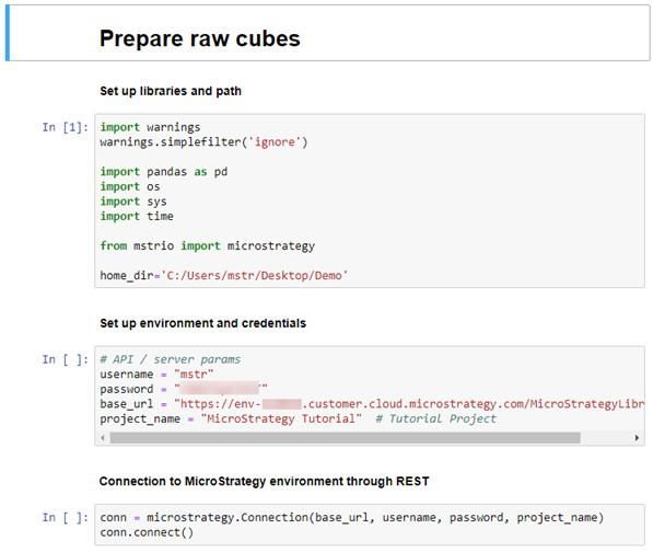
Import the cubes from MicroStrategy
Let’s examine the code as we execute the pieces of the script.
1 Locate the cell containing:
import warnings
warnings.simplefilter('ignore')
import pandas as
pd import os
import sys
import time
19 Walk-through: Modeling © 2018 MicroStrategy, Inc.
20 | MicroStrategyMicroStrategy World 2019 Workshop Book
Machine Learning Machine Learning
1
from mstrio import microstrategy
home_dir='C:/Users/mstr/Desktop/Demo'
The first two lines disable warnings so we won’t be distracted during this
workshop.
The next few lines initialize some of the libraries needed to create the
connection between the Intelligence Server and our server.
The next line loads the MicroStrategy mstrio library, which uses
MicroStrategy’s REST API to connect Python and the Intelligence Server.
The last line defines our home directory, the location we will run our files
from.
2 Execute the cell by pressing Shift+Enter, or click Run.
3 Locate the next cell containing:
# API / server
params username
= "mstr"
password =
"password"
base_url = "https://
env-
XXXXX.customer.cloud.microstrategy.com/
MicroStrategyLibrary/api"
project_name = "MicroStrategy Tutorial" #
Tutorial Project
Best This cell contains a series of variables used to connect to
Practice your Intelligence Server, including your user credentials. It is
a good practice to define variables this way, as changing
them will allow you to adapt the code to another
environment quickly.
© 2018 MicroStrategy, Inc. Walk-through: Modeling 20
MicroStrategy | 21Integrating Python Machine Learning Models and MicroStrategy
Machine Learning Machine Learning
1
4 Replace the password value with the password you received in your
MicroStrategy on AWS email.
5 Replace XXXXX with your environment number.
6 Execute the cell.
7 Locate the cell containing:
#conn = microstrategy.Connection(base_url=base_url,
username=username, password=password, project_name=
project_name)
conn = microstrategy.Connection(base_url, username,
password, project_name) conn.connect()
This sends a request to the MicroStrategy Intelligence Server establishing a
REST API connection between our machine learning server and the Intelligence
Server. The mstrio library takes care of managing the authentication token and
cookies needed to access the REST API server.
8 Execute the cell.
9 Locate the cell containing:
# Cubes to download cube_names = ['airlines',
'airports', 'states'] cube_ids =
['C983680C11E8D236B87F0080EF35FE86',
'EADC795811E8D236B83F0080EF15BE86',
'5946FA1211E8D237BB800080EFB5FF89']
This cell makes a list of the cube IDs that we need to download from the
MicroStrategy environment to our machine learning server. The objects’
values must be in the same order as their titles. For example, the first value in
cube_names is “airlines,” the first value of cube_ids must be the ID of the
airlines cube, and so on.
10 Execute the cell.
11 Locate the cell containing:
21 Walk-through: Modeling © 2018 MicroStrategy, Inc.
22 | MicroStrategyMicroStrategy World 2019 Workshop Book
Machine Learning Machine Learning
1
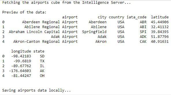
#Persist cubes on disk
for cube_id, cube_name in zip(cube_ids,
cube_names):
print("Fetching the " + cube_name + " cube from
the Intelligence Server..." + "\n") cube =
conn.get_cube(cube_id=cube_id)
cube.drop(labels=list(cube.filter(like='Row
Count')), inplace=True, axis=1) cube.columns =
cube.columns.str.lower() cube.columns =
cube.columns.str.replace(' ','_')
print("Preview of the data:")
print(cube.head()) print("\n")
time.sleep(3)
#Adjust for missing data
if cube_name=='airports':
cube.ix[cube.iata_code == 'ECP',
['latitude', 'longitude']] = "30.3416666667",
"-85.7972222222"
cube.ix[cube.iata_code == 'UST',
['latitude', 'longitude']] = "29.95861111",
"-81.33888888"
cube.ix[cube.iata_code == 'PBG',
['latitude', 'longitude']] = "44.65083", "-
73.46806"
print("Saving " + cube_name + " data
locally..."
+ "\n")
with
pd.HDFStore(os.path.join(home_dir,'Data\\
clean.h5')) as hdf:
hdf.append(key=cube_name, value=cube)
# Close MicroStrategy connection
conn.close()
© 2018 MicroStrategy, Inc. Walk-through: Modeling 22
MicroStrategy | 23Integrating Python Machine Learning Models and MicroStrategy
Machine Learning Machine Learning
1
This cell is long, so let’s split our explanation. Focusing on the following lines:
#Persist cubes on disk
for cube_id, cube_name in zip(cube_ids,
cube_names):
print("Fetching the " + cube_name + " cube from
the Intelligence Server..." + "\n") cube =
conn.get_cube(cube_id=cube_id)
cube.drop(labels=list(cube.filter(like='Row
Count')), inplace=True, axis=1) cube.columns =
cube.columns.str.lower() cube.columns =
cube.columns.str.replace(' ','_')
print("Preview of the data:")
print(cube.head()) print("\n")
time.sleep(3)
This is a loop that will iterate through the linked list of cube names and IDs.
A line will be printed in the notebook to tell us which cube is being retrieved.
The next line uses our conn object (our connection to MicroStrategy through
REST) to extract the cube data from the MicroStrategy Server into Python and
stored in a Python dataframe. Then the code drops row count values from
each row.
The next line sets every string in the cube’s column names in lowercase. After
that, we replace the spaces with underscore.
Then, three print statements offer us some feedback inside the notebook
itself. Note the use of the time.sleep() function. The sleep command waits
three seconds before moving on to the next cube. This is done deliberately to
allow us slow humans to read the output on screen. Focusing on the next
portion of this cell:
#Adjust for missing data
if cube_name=='airports':
cube.ix[cube.iata_code ==
23 Walk-through: Modeling © 2018 MicroStrategy, Inc.
24 | MicroStrategyMicroStrategy World 2019 Workshop Book
Machine Learning Machine Learning
1
'ECP', ['latitude',
'longitude']] =
"30.3416666667",
"-85.7972222222"
cube.ix[cube.iata_code == 'UST',
['latitude', 'longitude']] = "29.95861111",
"-81.33888888"
cube.ix[cube.iata_code == 'PBG',
['latitude', 'longitude']] = "44.65083", "-
73.46806"
This code executes within the for loop. For the airports cube, the code inserts
three specific values to correct some data quality errors. This is performed
here instead of at the source as you may not always have access to the source
data.
The next few lines in the cell are as follows:
print("Saving " + cube_name + " data
locally..."
+ "\n")
with pd.HDFStore(os.path.join(home_dir,'Data\\
clean.h5')) as hdf:
hdf.append(key=cube_name, value=cube)
This section warns the user that we are about to save the data from the
current cube to our server.
Finally, we write the file called clean.h5. Notice the way we used the home
directory path defined earlier and join it here. It is in an HDF5 format, a file-
based tabular format similar to the Hadoop native format.
The last lines of the cell are:
# Close MicroStrategy connection conn.close()
© 2018 MicroStrategy, Inc. Walk-through: Modeling 24
MicroStrategy | 25Integrating Python Machine Learning Models and MicroStrategy
Machine Learning Machine Learning
1
These lines terminate the API session after the data has been moved
successfully from the Intelligence Server to our machine learning server.
12 Execute the cell. Keep an eye on the output, as shown below:
25 Walk-through: Modeling © 2018 MicroStrategy, Inc.
26 | MicroStrategyMicroStrategy World 2019 Workshop Book
Machine Learning Machine Learning
1
13 In File Explorer, navigate to C:\Users\mstr\Desktop\Demo\Data to locate the
file clean.h5.
Notice the small size of the file—the data from our three cubes was not very large.
This will change with the flight data we are about to load.
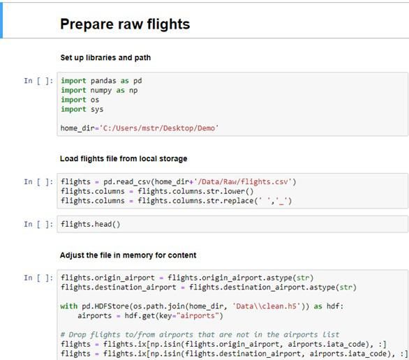
Import the local flights data
Our next notebook will walk us through loading a local file containing our flight data.
1 Return to the main Jupyter notebook tab.
2 Click 02_prep_raw_flights.ipynb.
The notebook opens as shown below.
© 2018 MicroStrategy, Inc. Walk-through: Modeling 26
MicroStrategy | 27Integrating Python Machine Learning Models and MicroStrategy
Machine Learning Machine Learning
1
Let’s walk through the cells and execute them together.
3 Locate the cell containing the following code:
import pandas as
pd import numpy as
np import os
import sys
home_dir='C:/Users/mstr/Desktop/Demo'
As before, this cell imports a few necessary libraries, including Pandas and
numpy, to be used in our code, as well as setting our home directory. We are
not loading mstrio here, as this data is not located on an Intelligence Server.
4 Execute the cell.
27 Walk-through: Modeling © 2018 MicroStrategy, Inc.
28 | MicroStrategyMicroStrategy World 2019 Workshop Book
Machine Learning Machine Learning
1
5 Locate the cell containing this code:
flights = pd.read_csv(home_dir+'/Data/Raw/
flights.csv') flights.columns =
flights.columns.str.lower()
flights.columns = flights.columns.str.replace('
','_')
The first line retrieves the data from the file stored locally in a CSV file.
The next two lines make every column name lower case and replaces spaces
with underscores. A warning is displayed; you can ignore it.
6 Execute the cell.
7 Locate the cell containing:
flights.head()
This line displays a few rows from the flights dataset in the notebook.
8 Execute the line.
The output below the cell should look like the image below:
9 Locate the cell containing this code:
© 2018 MicroStrategy, Inc. Walk-through: Modeling 28
MicroStrategy | 29Integrating Python Machine Learning Models and MicroStrategy
Machine Learning Machine Learning
1
flights.origin_airport =
flights.origin_airport.astype(str)
flights.destination_airport =
flights.destination_airport.astype(str)
with pd.HDFStore(os.path.join(home_dir,
'Data\\ clean.h5')) as hdf: airports =
hdf.get(key="airports")
# Drop flights to/from airports that are not in the
airports list
flights =
flights.ix[np.isin(flights.origin_airport,
airports.iata_code), :]
flights =
flights.ix[np.isin(flights.destination_airport,
airports.iata_code), :]
# Drop (6) flights without scheduled time
flights =
flights.ix[np.isnan(flights.scheduled_time)==False,
:]
# Add a unique ID for each flight
flights['FL_ID'] = ["FL_" + str(x) for x in
np.arange(0, len(flights))]
# Delete critical future leak. Do not give model info
it is looking for.
drop_cols = ['departure_time', 'taxi_out',
'wheels_off', 'elapsed_time', 'air_time',
'wheels_on', 'taxi_in', 'arrival_time',
'arrival_delay', 'diverted',
'cancellation_reason', 'air_system_delay',
'security_delay', 'airline_delay',
'late_aircraft_delay', 'weather_delay', 'year',
'tail_number']
29 Walk-through: Modeling © 2018 MicroStrategy, Inc.
30 | MicroStrategyMicroStrategy World 2019 Workshop Book
Machine Learning Machine Learning
1
flights.drop(drop_cols, inplace=True, axis=1)
Let’s digest this long cell in smaller chunks. Focus on the following lines:
flights.origin_airport =
flights.origin_airport.astype(str)
flights.destination_airport =
flights.destination_airport.astype(str)
These lines change the data type of the origin and destination airports into text
data, known as strings, to ensure they retain their original format.
with pd.HDFStore(os.path.join(home_dir, 'Data\\
clean.h5')) as hdf: airports =
hdf.get(key="airports")
These lines retrieve the airports table from the clean.h5 file we saved in the
previous script.
# Drop flights to/from airports that are not in the
airports list
flights =
flights.ix[np.isin(flights.origin_airport,
airports.iata_code), :]
flights =
flights.ix[np.isin(flights.destination_airport,
airports.iata_code), :]
These lines use the airports codes to keep only the flights related to the
airports in the table.
# Drop (6) flights without scheduled time
flights =
flights.ix[np.isnan(flights.scheduled_time)==False,
:]
© 2018 MicroStrategy, Inc. Walk-through: Modeling 30
MicroStrategy | 31Integrating Python Machine Learning Models and MicroStrategy
Machine Learning Machine Learning
1
This line removes flights that do not have a scheduled time listed, so our dataset
doesn’t have incomplete data.
flights['FL_ID'] = ["FL_" + str(x) for x in
np.arange(0, len(flights))]
This line iterates over the flights table and adds a new identifier for each flight
in the FL_ID column.
# Delete critical future leak. Do not give model info
it is looking for.
drop_cols = ['departure_time', 'taxi_out',
'wheels_off', 'elapsed_time', 'air_time',
'wheels_on', 'taxi_in',
'arrival_time', 'arrival_delay', 'diverted',
'cancellation_reason',
'air_system_delay', 'security_delay',
'airline_delay',
'late_aircraft_delay',
'weather_delay',
'year', 'tail_number']
flights.drop(drop_cols, inplace=True, axis=1)
These lines delete the listed columns from the flight dataset. These columns
contain information about the flights that will bias the model. These variables
are often called “future leaks.”
10 Execute the cell. It may take a few minutes to run.
11 Locate the cell containing:
with pd.HDFStore(os.path.join(home_dir,
'Data\\ clean.h5')) as hdf:
hdf.append(key="flights", value=flights)
This cell commits the new flights table and appends it to the clean.h5 file we
have locally.
31 Walk-through: Modeling © 2018 MicroStrategy, Inc.
32 | MicroStrategyMicroStrategy World 2019 Workshop Book
Machine Learning Machine Learning
1
12 Execute the cell. Saving may take a few moments because the data is large.
13 Click Kernel, then click Shutdown. Confirm the shutdown.
14 Close the browser tab.
15 In File Explorer, locate the clean.h5 file.
Data preparation
When we train a model, typically we use a single table that contains all of the data
we want the model to use. In that table, we add features—new data that wasn’t
present in the raw data—that reflect our knowledge of the business problem or
our hypotheses about what is correlated with the business problem.
This is done through joins, transformations, merges, and lookups using the
available data sources.
As an example, our Flights table had the origin and destination airports, and our
Airports data contained the latitude and longitude for each airport. We want to
use the latitude and longitude in our model, in case there’s a relationship between
those variables and the outcome for each flight.
To do that, we have to join airports with flights.
After we do this a couple times, we end up with a very large table. In this case, we
have our 5 million flights, accompanied by 190 columns! In total these columns
reflect all of our ideas, hypotheses, and thoughts we want the model to learn from
to understand what causes flights to be delayed.
© 2018 MicroStrategy, Inc. Walk-through: Modeling 32
MicroStrategy | 33Integrating Python Machine Learning Models and MicroStrategy
Machine Learning Machine Learning
1
Prepare the data
1 On the main Jupyter Notebook page, click
03_prep_training. The notebook will open.
Rather than running each cell individually, we will run the entire script to
save time. Please see the Appendix for individual steps.
2 In the Cell menu, select Run All.
3 Once completed, click Kernel, then click Shutdown. Confirm the
shutdown.
4 Close the browser tab.
Data splitting
This is the last step in data preparation.
33 Walk-through: Modeling © 2018 MicroStrategy, Inc.
34 | MicroStrategyMicroStrategy World 2019 Workshop Book
Machine Learning Machine Learning
1
We divide our data into different sets:
• We need to create a partition of the data to use for training the model. This is
the data the machine learning algorithm uses to fit the model.
• We also need a test set. The test set is used to evaluate the quality of the
model after it has been trained with an objective metric like r-squared or root
mean squared error.
• The final set is the validation set. The validation set serves a similar purpose to
the test set. It is used to provide a confirmation that the error rate from both
the validation set and the test set are similar.
The purpose of the training-test split is to estimate the reliability of our model
when using unseen data. We do this to get a sense of how well our model will
perform when it’s in production.
Another way of doing this is through cross-validation, where this train-test-
validation splitting process is repeated numerous times, and produces a distribution
of error estimates instead of a single error estimate.
In thjs case, we’ll do a random split of the data. About 65% of the data is used for
training, and the remaining data is split evenly across the test and validation sets.
Due to time limitations for this workshop, we will use smaller sets to train and
evaluate the data. Normally the model would use the entirety of the data.
Split the data
1 Locate the following cell:
© 2018 MicroStrategy, Inc. Walk-through: Modeling 34
MicroStrategy | 35Integrating Python Machine Learning Models and MicroStrategy
Machine Learning Machine Learning
1
# ########################### #
# Train-Test-Validation Split #
# ########################### #
prod = flights[np.logical_and(flights.month == 12,
flights.day == 31)]
flights = flights[~np.logical_and(flights.month ==
12, flights.day == 31)]
train, test = train_test_split(flights, test_size=
0.35) test, oos = train_test_split(test,
test_size=0.5)
This cell creates our train, test, and validation splits. You see the creation of
the train and test sets, followed by a split of the test dataset to create the
validation set. Additionally, a data frame called prod is created, which will
represent the data our model will not see: these are all the flights for
December 31st. We will use this data later in the workshop as an out of
sample test.
2 Execute this cell. This may take a few moments.
3 Locate the cell containing the following:
# ############# #
# Store in HDF5 #
# ############# #
with pd.HDFStore(os.path.join(home_dir, 'Data\\
ready.h5')) as hdf:
hdf.append(key="train", value=train)
hdf.append(key="test", value=test)
hdf.append(key="oos", value=oos)
hdf.append(key="prod", value=prod)
Now that we have some data prepared, we will store in our home directory, so
it can be modified later if needed.
4 Execute this cell. Saving may take a few moments.
5 Click Kernel, then click Shutdown. Confirm the shutdown.
35 Walk-through: Modeling © 2018 MicroStrategy, Inc.
36 | MicroStrategyMicroStrategy World 2019 Workshop Book
Machine Learning Machine Learning
1
6 Close the browser tab.
7 In the File Explorer, locate the ready.h5 file and notice the file is now two and
a half gigabytes.
Walkthrough: Modeling
In the modeling phase, you select an algorithm or collection of algorithms suitable
for our problem. Thanks to our earlier work, the data is structured for use in our
machine learning algorithms, but we might not know exactly what algorithm is
going to work the best.
Classes of machine learning problems
There are three main classes of machine learning algorithms, which are
represented in the diagram below:
© 2018 MicroStrategy, Inc. Walk-through: Modeling 36
MicroStrategy | 37Integrating Python Machine Learning Models and MicroStrategy
Machine Learning Machine Learning
1
• Unsupervised learning algorithms are used most often for pattern discovery,
including, for example, when you have data but aren’t exactly sure what
question is being asked.
• Supervised learning algorithms are used when we want to infer a relationship
between input and output pairs. They comprise many of the applications
you’ve probably read about. For example, supervised learning tasks include
regression analysis and data classification. Unlike unsupervised learning, these
tasks require labeled data. In other words, we must know the true outcome
for each record in our dataset.
• Reinforcement learning algorithms are intended to optimize performance
outcomes. Unlike supervised learning algorithms, they do not require the
correct input and output pairs. They are used in many industrial and software
applications, including in manufacturing and automation.
Neural networks
Since we are trying to predict whether a flight is likely to be on time, delayed, or
canceled, and we have labeled data, we are now working on a supervised learning
problem classification. To do so, we will use a neural network.
Neural networks are one of the most important machine learning techniques. As
diagram below shows, a neural network consists of three parts:
1. An input layer, composed of the labeled real-world observations from our
dataset, such as origin airport and departure time.
2. An output layer, which contains our predictions regarding the probable
status of a flight given its input characteristics.
3. Multiple hidden layers, composed of sequential algorithms that analyze
and process data from the input layer and previous layers in order to
generate the outputs. Because we are using multiple hidden layers, this is a
deep learning model.
37 Walk-through: Modeling © 2018 MicroStrategy, Inc.
38 | MicroStrategyMicroStrategy World 2019 Workshop Book
Machine Learning Machine Learning
1
To use our neural network, we must first “train” it. We do so by feeding input
layer data into an activation function. The hidden layers of the neural network will
then automatically perform a series of calculations to tune the weights of each
node in the network, ensuring that the output layer most closely matches the true
output that we observed in our data—in other words, making sure that our model
produces the most accurate predictions possible.
Train the model
To train our model, we start in our 04_train.ipnyb notebook.
1 On the Jupyter notebook main page, click 04_train.
The notebook opens.
2 Locate the cell at the top containing the following code:
© 2018 MicroStrategy, Inc. Walk-through: Modeling 38
MicroStrategy | 39Integrating Python Machine Learning Models and MicroStrategy
Machine Learning Machine Learning
1
# package imports
import sys import
os import gc
import numpy as
np import pandas
as pd import
pickle
from keras.models import Sequential from
keras.layers.core import Dense, Dropout
from keras.layers.normalization
import BatchNormalization from
keras.callbacks import EarlyStopping
from keras import regularizers
from sklearn.preprocessing import MaxAbsScaler
Next, load the packages that we need in order to train our model. You will
receive some warnings from TensorFlow, but you can safely ignore them.
3 Execute this cell.
4 Locate the cell containing the following code:
# helper function for returning the target
variables from the training data def
get_targets(df):
targets = ['cancelled', 'delayed',
'on_time']
return df.filter(items=targets,
axis=1)
This contains a support function we will use later. It returns the target
variables when we run the model.
5 Execute this cell.
39 Walk-through: Modeling © 2018 MicroStrategy, Inc.
40 | MicroStrategyMicroStrategy World 2019 Workshop Book
Machine Learning Machine Learning
1
6 Locate the cell containing the following code:
# helper function for dropping columns that
we do not wish to train the model on def
drop_cols(df):
drop = ['month', 'day', 'day_of_week',
'airline', 'flight_number', 'iata_code_orig',
'state_orig', 'iata_code_dest',
'state_dest', 'origin_airport',
'destination_airport', 'scheduled_departure',
'departure_delay', 'scheduled_time',
'distance',
'scheduled_arrival', 'FL_ID',
'cancelled', 'delayed', 'on_time']
return df.drop(drop, axis=1)
This cell also contains a support function. It removes, or “drops,” some
columns from a data frame that we do not need.
7 Execute this cell.
8 Locate the cell containing the following code:
# set home directory home_dir =
"C:\\Users\\mstr\\Desktop\\Demo"
# set seed for reproducibility
np.random.seed(91919)
In this cell, we define the path to our files and set a defined seed number that
will allow us to reproduce the same results every time. This is because the
activation function starts with a pseudo-random value that we can choose.
9 Execute this cell.
10 Locate the cell containing the following code:
© 2018 MicroStrategy, Inc. Walk-through: Modeling 40
MicroStrategy | 41Integrating Python Machine Learning Models and MicroStrategy
Machine Learning Machine Learning
1
# ################ #
# Load in the data
# #
################ #
with pd.HDFStore(os.path.join(home_dir,
'Data\\ ready.h5')) as hdf:
train = hdf.get(key="train")
test = hdf.get(key="test")
This cell loads in our training data as well as in our test data.
11 Execute this cell. Note that these datasets are quite large, so you should not be
concerned if they take time to load.
12 Locate the cell containing the following:
# ######### #
# Data prep #
# ######### #
if True:
# To speed-up model training, we're taking a
subset of the data
# If you want to train the full model set the
previous line 'False'
train, test = [df.sample(n=25000) for df in
[train, test]]
# x-vars and y-vars
x_train, x_test = [np.array(drop_cols(df=df)) for
df in [train, test]]
y_train, y_test = [np.array(get_targets(df=df)) for
df in [train, test]]
*Note that if this condition is set to True, the set is limited to 25,000
rows. To train on the complete data frame, you should set this condition
to False.
41 Walk-through: Modeling © 2018 MicroStrategy, Inc.
42 | MicroStrategyMicroStrategy World 2019 Workshop Book
Machine Learning Machine Learning
1
We’ll use a subset of our data to train and test our model. Depending on the
application and the dataset, neural networks can exhibit a lot of variation in
the time they take to fit a model. By only using a sample of the data, we can
ensure that this process will only take a few minutes.
We also want to manage the program’s memory profile as it runs. The more
data we want analyze, the more system resources the program must
consume.
13 Execute this cell. By doing so, we split our data into x and y sets. The x set
contains the input observations that the model will use to learn from. The y set
contains the outcome observations.
14 Locate the cell containing the following code:
# ####### #
# Scaling # # ####### # scaler =
MaxAbsScaler() x_train =
scaler.fit_transform(x_train)
x_test = scaler.transform(x_test)
# clean-up
del train,
test
gc.collect()
This cell scales our values to make them proportionally smaller so they are
easier to calculate.
Note that gc.collect is a garbage collection command used here to help reduce
memory usage.
15 Execute this cell.
16 Locate the cell containing the following code:
# ############################ #
© 2018 MicroStrategy, Inc. Walk-through: Modeling 42
MicroStrategy | 43Integrating Python Machine Learning Models and MicroStrategy
Machine Learning Machine Learning
1
# Configure the neural network # #
############################ # dnn = Sequential()
dnn.add(Dense(1024, input_dim=190,
activation='relu',
kernel_initializer='uniform',
bias_initializer='normal',
kernel_regularizer=
regularizers.l2(0.001),
43 Walk-through: Modeling © 2018 MicroStrategy, Inc.
44 | MicroStrategyMicroStrategy World 2019 Workshop Book
Machine Learning Machine Learning
1
activity_regularizer=
regularizers.l2(0.001)))
dnn.add(Dropout(0.2))
dnn.add(Dense(512,
activation='tanh',
kernel_initializer='normal',
bias_initializer='uniform',
kernel_regularizer=
regularizers.l2(0.001),
activity_regularizer=
regularizers.l2(0.01)))
dnn.add(BatchNormalization())
dnn.add(Dropout(0.2))
dnn.add(Dense(128,
activation='relu',
kernel_initializer='zeros',
bias_initializer='uniform',
kernel_regularizer=
regularizers.l2(0.001),
activity_regularizer=
regularizers.l2(0.1)))
dnn.add(BatchNormalization())
dnn.add(Dense(3,
activation='softmax',
kernel_initializer='normal',
bias_initializer='ones'))
dnn.compile(loss='categorical_crossentropy',
optimizer='adagrad',
metrics=['categorical_accuracy'])
© 2018 MicroStrategy, Inc. Walk-through: Modeling 44
MicroStrategy | 45Integrating Python Machine Learning Models and MicroStrategy
Machine Learning Machine Learning
1
earlystopping = EarlyStopping(monitor='val_loss',
min_delta=0, patience=0, verbose=0, mode='auto')
This cell configures the parameters of our neural network, which we must do
in order to initialize its structure.
Notice the parameter beginning with dnn.add(Dense. This sets the number of
nodes in each layer: from 1024, to 512, and ultimately down to 3. The selection
of this “network topology” is a common area of debate. Data scientists typically
spend a long time selecting and fine tuning these kinds of parameters.
17 Execute this cell.
18 Locate the cell containing the following:
# ######## #
# Training # # ######## # dnn.fit(x=x_train,
y=y_train, batch_size=2500,
epochs=10, verbose=True,
validation_data=(x_test, y_test),
callbacks=[earlystopping])
This cell will initiate the training of our neural network. You should see
notifications in the console informing you of what is happening as the model
attempts to optimize and achieve the lowest lost statistic. These notifications
will look something like this:
Note that as each training “epoch” is completed the loss statistic declines. This
means our model is becoming a more accurate predictor compared to
previous iterations.
19 Open the Task Manager (right click the taskbar and click Task Manager).
45 Walk-through: Modeling © 2018 MicroStrategy, Inc.
46 | MicroStrategyMicroStrategy World 2019 Workshop Book
Machine Learning Machine Learning
1
20 Keep an eye on the name Python in the Processes tab.
This provides a preview of the CPU and memory resources that our
calculations are consuming. In general, this demand will scale with amount of
data we are trying to process. More demanding tasks, in other words, require
more system resources.
Note that training the model will require significant CPU resources. Indeed,
you should not be surprised to see Python frequently utilizing close to 100% of
those available.
21 Execute the cell from Step 19. This will take a few minutes.
22 Locate the cell containing the following code:
# ############ #
# Save to disk #
# ############ #
© 2018 MicroStrategy, Inc. Walk-through: Modeling 46
MicroStrategy | 47Integrating Python Machine Learning Models and MicroStrategy
# save the model and pre-processing scaler to
disk
dnn.save(os.path.join(home_dir, 'Data\Model\
dnn_weights.h5'))
pickle.dump(scaler,
open(os.path.join(home_dir,
'Data\Model\dnn_scaler.pkl'), 'wb'))
Once the model is trained, we must save it somewhere. This cell does so in
your home directory’s model subfolder of the data folder.
23 Execute this cell. Saving may take a few moments.
24 Click Kernel, then click Shutdown. Confirm the shutdown.
25 Close the browser tab.
26 In File Explorer, locate the Model folder. You should see two saved model files,
as shown below:
• “dnn_scaler.pkl” contains the scaler, a pre-processing utility used to
structure the data for the neural network.
• “dnn_weights.h5” contains the weights of the neural network.
Walkthrough: Evaluation
Now that we have trained our model, we can evaluate how well it predicts flight
departure status.
To help with the discussion, we have calculated the Area Under the Curve (AUC)
statistic for the model on each of the outcomes. We have used this statistic to plot
the Receiver Operating Characteristics (ROC), which visualizes the ratio of true
positives (correctly predicted examples) to false positives (incorrectly predicted
examples). An excellent model should look like a sharp curve approaching the
© 2018 MicroStrategy, Inc. 47
48 | MicroStrategyMicroStrategy World 2019 Workshop Book
upper left-hand corner of the graph. The dashed line is a reference point for a
model that randomly guesses the outcome.
The first ROC graph visualizes the AUC for the canceled flights. The model’s AUC
score of 0.71 means it did much better than random guesses. A more accurate
model would have an AUC score even closer to 1, and have a curve more sharply
sloped towards the upper left-hand corner of the graph.
Next, we have the AUC for delayed flights, which came in at 0.64.
And finally, we have the AUC for on-time flights which was also 0.64.
© 2018 MicroStrategy, Inc. 48
MicroStrategy | 49Integrating Python Machine Learning Models and MicroStrategy
Machine Learning
Before putting these models into production, we want to spend more time
comprehensively assessing the performance of the model under a number of
different assumptions.
Let’s assume for this workshop that we have successfully tested this model.
Congratulations! You just trained a model in Python.
Let’s now use this model to predict departure statuses for flights that we have not
yet observed.
Predict flight status
We’ll use our previously trained neural network to predict the departure status of
unobserved flights. To do this, we’ll open our 05_predict.ipynb script. This script
acquires the new data, applies the neural network to the new data, and then creates
a cube containing predictions inside of MicroStrategy, which we can use inside a
dossier or dashboard.
1 In the Jupyter notebook main page, click 05_predict.
The notebook should now open and you should see the following:
2 Locate the cell at the top containing the following code:
import pandas as pd import numpy as np
import os import sys import gc import
pickle from keras.models import load_model
49 © 2018 MicroStrategy, Inc.
50 | MicroStrategyMicroStrategy World 2019 Workshop Book
from mstrio import microstrategy
This cell will import the libraries we need for the notebook. Notice the return of
mstrio, as we will be interacting with MicroStrategy towards the end of this
phase.
3 Execute this cell.
4 Locate the cell containing the following:
# helper function for returning the target variables
from the training data def get_targets(df):
targets = ['cancelled', 'delayed',
'on_time']
return df.filter(items=targets,
axis=1)
This filters out the dependent variables (“cancelled,” “delayed,” and “on
time”) from our test dataset.
5 Execute this cell.
6 Locate the cell containing the following code:
# helper function for dropping columns that we do
not wish to train the model on def drop_cols(df):
drop = ['month', 'day', 'day_of_week',
'airline', 'flight_number', 'iata_code_orig',
'state_orig', 'iata_code_dest',
'state_dest', 'origin_airport',
'destination_airport', 'scheduled_departure',
'departure_delay', 'scheduled_time',
'distance', 'scheduled_arrival', 'FL_ID',
'cancelled', 'delayed', 'on_time']
return df.drop(drop, axis=1)
This cell will drop columns that we do not wish to use when training our
model.
© 2018 MicroStrategy, Inc. 50
MicroStrategy | 51Integrating Python Machine Learning Models and MicroStrategy
Machine Learning
7 Execute this cell.
8 Locate the cell containing the following code:
# set home directory home_dir =
"C:\\Users\\mstr\\Desktop\\Demo"
# set seed for reproducibility
np.random.seed(91919)
In this cell, we set our path to our files and set the initializing pseudo-random
seed. Note that you are using the same number as before.
9 Execute this cell.
10 Locate the cell containing the following code:
# ######################################### #
# Load in the network and data
preprocessor # #
#########################################
#
dnn =
load_model(filepath=os.path.join(home_dir,
'Data\Model\dnn_weights.h5'))
scaler =
pickle.load(open(os.path.join(home_dir,
'Data\Model\dnn_scaler.pkl'), 'rb'))
This cell will load in the model weights and the pre-processor scaler.
11 Execute this cell.
12 Locate the cell containing the following code:
51 © 2018 MicroStrategy, Inc.
52 | MicroStrategyYou can also read