Reynolds-Averaged Navier-Stokes Computations of the NASA Juncture Flow Model Using FUN3D and OVERFLOW

Page created by Nicole Fisher
 
CONTINUE READING
Reynolds-Averaged Navier-Stokes Computations of the NASA Juncture Flow Model Using FUN3D and OVERFLOW
AIAA SciTech Forum                                                                                                                                            10.2514/6.2020-1304
                                                                              6-10 January 2020, Orlando, FL
                                                                              AIAA Scitech 2020 Forum

                                                                                                                 Reynolds-Averaged Navier-Stokes Computations of the NASA
                                                                                                                    Juncture Flow Model Using FUN3D and OVERFLOW

                                                                                                                                                                               C. L. Rumsey∗
                                                                                                                                                     NASA Langley Research Center, Hampton, VA 23681
                                                                                                                                                                                 H. C. Lee†
                                                                                                                                                   Science and Technology Corp., Moffett Field, CA 94035
                                                                                                                                                                               T. H. Pulliam‡
Downloaded by NASA LANGLEY RESEARCH CENTRE on April 14, 2020 | http://arc.aiaa.org | DOI: 10.2514/6.2020-1304

                                                                                                                                                    NASA Ames Research Center, Moffett Field, CA 94035

                                                                                                                          Two Reynolds-averaged Navier-Stokes codes, FUN3D and OVERFLOW, are used to assess the capability
                                                                                                                      of Spalart-Allmaras-based turbulence models to predict the flow over the NASA Juncture Flow model. Both
                                                                                                                      free-air and in-tunnel simulations are performed. While the tunnel walls have some influence, it is found to be
                                                                                                                      relatively minor in the juncture region of interest. Results from the two codes are found to be consistent with
                                                                                                                      each other in attached flow regions, but results in the area of separation still show grid and code sensitivity,
                                                                                                                      even on grids as large as 400 million unknowns. Nonetheless, it is possible to draw conclusions regarding the
                                                                                                                      model capabilities. Without a quadratic constitutive relation, the linear model predicts a separation size that
                                                                                                                      is too large. The inclusion of a nonlinear quadratic constitutive relation improves results significantly, but
                                                                                                                      separation still occurs too far upstream. Predictions of turbulent normal stress differences play a key role in
                                                                                                                      this flow. Although the nonlinear model makes better predictions in this regard, they could still be improved,
                                                                                                                      particularly in the streamwise normal component near the wall.

                                                                                                                                                                          I.     Introduction
                                                                                                                     CFD is considered to be unreliable in its prediction of separated flows in junction regions, such as those that can
                                                                                                                occur near the trailing edge of an aircraft wing near its intersection with the fuselage. This type of flow feature may
                                                                                                                influence or contribute to aircraft stall, so it is important to learn specifically how CFD methods are deficient, and to
                                                                                                                try to improve them if possible. The NASA Juncture Flow (JF) experiment was designed to study this type of flow
                                                                                                                phenomenon for the purpose of CFD validation. The experiment, conducted in the NASA Langley Research Center
                                                                                                                14- by 22-Foot Subsonic Tunnel (14x22), provides flowfield data (velocity, Reynolds stresses, and velocity triple
                                                                                                                products) in and near the wing-body junction region, along with boundary condition and geometry information so that
                                                                                                                CFD validation can be confidently performed. Ultimately, the goal is to learn how well existing CFD methods predict
                                                                                                                the flowfield features in (and leading up to) the corner region, and to gain enough insight to be able to improve the
                                                                                                                methods as needed. The initial focus is on Reynolds-averaged Navier Stokes (RANS) turbulence models, but future
                                                                                                                efforts will focus on scale-resolving simulations as well.
                                                                                                                     The flow physics of wing-body juncture flows is quite complex [1, 2]. In addition to the typical presence of a
                                                                                                                horseshoe-type vortex wrapping around the wing leading edge, there also may be a smaller secondary corner vortex
                                                                                                                initiated by gradients of the Reynolds stresses [3]. These vortices influence the flowfield in the junction region.
                                                                                                                Experimentally, Simpson and coauthors have investigated juncture flows in great detail [4]. However, that body of
                                                                                                                work did not include much focus on trailing-edge corner separation. More recently, ONERA conducted a series of
                                                                                                                separated juncture flow investigations, involving both experiment and CFD. Gand et al. [1, 5, 6] described a simplified
                                                                                                                wing-body juncture experiment that used an NACA 0012 wing mounted to a flat plate. Although designed to achieve
                                                                                                                a corner separation, the flow in the wind tunnel experiment remained attached. Subsequently, the investigators re-
                                                                                                                designed the experiment with a twisted NACA 0015 wing on a plate [7], for which the corner flow separated.
                                                                                                                  ∗ Senior Research Scientist, Computational AeroSciences Branch, Mail Stop 128, Fellow AIAA.
                                                                                                                  † Research Scientist, Computational Aerosciences Branch, Mail Stop 258-2, Member AIAA.
                                                                                                                  ‡ Senior Research Scientist, Computational Aerosciences Branch, Mail Stop 258-2, Associate Fellow AIAA.

                                                                                                                                                                                     1 of 31

                                                                              This material is declared a work of the U.S. Government and is not subject to copyright protection in the United States.
Reynolds-Averaged Navier-Stokes Computations of the NASA Juncture Flow Model Using FUN3D and OVERFLOW
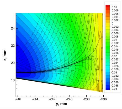
The NASA JF project underwent a significant amount of preparatory work [8–17], and has concluded its first wind
                                                                                                                tunnel test. The results are available in Kegerise and Neuhart [18], as well as on the NASA Turbulence Modeling
                                                                                                                Resource website [19]. Additional testing is planned in the future, to expand the breadth of the experimental data. The
                                                                                                                main focus of the experiment already performed was its use of a Laser Doppler Velocimetry (LDV) system carried on
                                                                                                                board the model to measure the junction flowfield. This system was installed inside the fuselage, and its lasers were
                                                                                                                emitted through side windows on the model. This setup allowed the collection of highly accurate flowfield data to
                                                                                                                within a very small distance of the junction corner.
                                                                                                                    A photograph of the NASA Juncture Flow model is shown in Fig. 1, along with an inset showing a surface oil flow
                                                                                                                photo of the corner separation at angle of incidence of 5◦ . Generally, the success or failure of CFD for this problem
                                                                                                                centers around its ability to predict this separation size (length and width) accurately as a function of the model’s angle
                                                                                                                of incidence. However, it is recognized that measuring separation extent with oil is inherently qualitative in nature;
                                                                                                                therefore, CFD results should be evaluated cautiously. On the other hand, the LDV data provide quantitative measures
                                                                                                                of flowfield details, so we expect to learn a great deal from comparisons between CFD and experiment. The model
                                                                                                                itself had a fuselage length of 4.839 m with a wingspan of 3.397 m (tip to tip). The wing had a leading edge sweep of
Downloaded by NASA LANGLEY RESEARCH CENTRE on April 14, 2020 | http://arc.aiaa.org | DOI: 10.2514/6.2020-1304

                                                                                                                27.1◦ , and for all the investigations in this paper a leading edge fillet or horn was included on the wing to mitigate the
                                                                                                                formation of a strong horseshoe vortex. A coordinate system was chosen with (x, y, z) = (0, 0, 0) at the model nose
                                                                                                                with the x-axis running downstream along the center axis of the fuselage, z up, and y out the starboard wing. The
                                                                                                                fuselage had flat sides, located at y = ±236.098 mm. The wing trailing edge at the root was at x = 2961.929 mm.
                                                                                                                    Two previous papers [16, 17] detailed initial RANS CFD comparisons with the experimental data, using the codes
                                                                                                                FUN3D [20] and OVERFLOW [21], respectively. These two CFD codes were also involved extensively throughout
                                                                                                                the project, helping to design the experiment. In this paper, the general capabilities of one class of turbulence model
                                                                                                                (based on Spalart-Allmaras [22]) for predicting juncture flow separation are summarized using the same two codes.
                                                                                                                The following section outlines the numerical methods, turbulence model specifics, and problem setup. Then, results
                                                                                                                are provided, which include free-air grid refinement studies, separation predictions, surface pressure predictions, and
                                                                                                                flowfield predictions. The influence of wind tunnel walls in CFD predictions are also discussed. Finally, conclusions
                                                                                                                are given.

                                                                                                                                               II.    Numerical Methods and Problem Setup
                                                                                                                   The CFD codes FUN3D and OVERFLOW are briefly described in this section, along with the turbulence models
                                                                                                                and grids employed. The flow conditions are also given.

                                                                                                                A.   FUN3D
                                                                                                                The NASA FUN3D [23,24] solver is an unstructured three-dimensional, implicit, Navier-Stokes code that is nominally
                                                                                                                second-order spatially accurate. Roe’s flux difference splitting [25] is used for the calculation of the inviscid terms for
                                                                                                                all the results in this paper (other flux construction methods are also available). The use of flux limiters are grid and
                                                                                                                flow dependent (none were used here). Other details regarding the code can be found in the extensive bibliography
                                                                                                                that is accessible at the FUN3D website [20].
                                                                                                                     For the free-air computations, a farfield Riemann invariant boundary condition was imposed on the outer boundary,
                                                                                                                no-slip solid wall boundary conditions were applied on the model, and symmetry conditions were used on the x-z
                                                                                                                symmetry plane. For in-tunnel runs, no-slip solid wall boundary conditions were applied on the model and inviscid slip
                                                                                                                wall boundary conditions were applied on the tunnel walls. Also, a proportional-integral-derivative (PID) controller
                                                                                                                was employed for automatically adjusting the tunnel back pressure at user-defined intervals in order to attain the
                                                                                                                desired flow conditions, as described for the 14x22 in Carlson [26]. The frequency of the update depends on the lag
                                                                                                                time of the particular simulation. The test cases in this paper used an update frequency of 1000 iterations. The tunnel
                                                                                                                inflow conditions were constant total pressure and total temperature across the inflow face upstream of the tunnel
                                                                                                                contraction.
                                                                                                                     Typical results on the fine grid level were computed on 2744 Intel Broadwell cores and utilized approximately 25
                                                                                                                hours of walltime.

                                                                                                                B.   OVERFLOW
                                                                                                                OVERFLOW is a NASA developed RANS solver. It uses structured overset grids to simulate fluid flow. All of
                                                                                                                the OVERFLOW cases were run with OVERFLOW 2.2O. The 3rd -order Roe upwind scheme [25] was used for the
                                                                                                                convective fluxes, and the implicit solve was done using the ARC3D Beam-Warming scalar pentadiagonal scheme

                                                                                                                                                                          2 of 31
Reynolds-Averaged Navier-Stokes Computations of the NASA Juncture Flow Model Using FUN3D and OVERFLOW
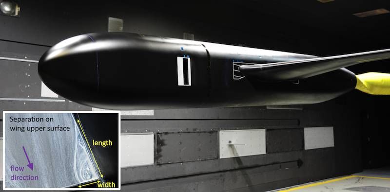
and low-Mach preconditioning [21]. Similar to FUN3D, free-air computations employed a farfield Riemann invariant
                                                                                                                boundary condition imposed on the outer boundaries, and no-slip solid wall boundary conditions were applied on
                                                                                                                the model. OVERFLOW simulations were performed for the full model, i.e., no symmetry plane assumption. For
                                                                                                                in-tunnel runs, no-slip solid wall boundary conditions were applied on the model and tunnel walls in the test section.
                                                                                                                A slip wall boundary condition was applied on the tunnel walls downstream of the test section in the diffuser region to
                                                                                                                improve the downstream boundary condition implementation [14]. Typical free-air results were computed using 280
                                                                                                                Intel Broadwell cores, and utilized approximately 12 hours of walltime. The wind tunnel simulations used 800 Intel
                                                                                                                Skylake Cores, for anywhere between 60 to 120 hours of walltime. The wind tunnel simulations took longer to run
                                                                                                                due to the need to iterate the back pressure to get the tunnel conditions to match.

                                                                                                                C.     Turbulence Models Employed
                                                                                                                For all the cases in this paper, the CFD codes were run “fully turbulent” (no laminar regions or transition were en-
                                                                                                                forced). In the experiment, the fuselage and wing upper and lower surfaces had boundary layer trips applied.
Downloaded by NASA LANGLEY RESEARCH CENTRE on April 14, 2020 | http://arc.aiaa.org | DOI: 10.2514/6.2020-1304

                                                                                                                1.    SA-RC
                                                                                                                The Spalart-Allmaras turbulence model with Rotation-Curvature correction [27] is the “base” model employed in this
                                                                                                                study. It is a linear one-equation RANS turbulence model given by:

                                                                                                                                                                                  2                                       
                                                                                                                      ∂ ν̂      ∂ ν̂                          h        cb1 i      ν̂    1 ∂             ∂ ν̂         ∂ ν̂ ∂ ν̂
                                                                                                                           + uj      = cb1 (fr1 − ft2 )Ŝ ν̂ − cw1 fw − 2 ft2         +        (ν + ν̂)        + cb2                (1)
                                                                                                                      ∂t        ∂xj                                    κ          d     σ ∂xj           ∂xj          ∂xi ∂xi

                                                                                                                where the turbulence eddy viscosity is computed from

                                                                                                                                                                       µt = ρν̂fv1                                                  (2)
                                                                                                                and

                                                                                                                                                                                    χ3
                                                                                                                                                                    fv1 =                                                           (3)
                                                                                                                                                                               χ3   + c3v1
                                                                                                                                                                                    ν̂
                                                                                                                                                                           χ=                                                       (4)
                                                                                                                                                                                    ν
                                                                                                                                                                                  ν̂
                                                                                                                                                                  Ŝ = Ω +             fv2                                          (5)
                                                                                                                                                                                 κ2 d2
                                                                                                                                                                                    χ
                                                                                                                                                                 fv2 = 1 −                                                          (6)
                                                                                                                                                                                 1 + χfv1
                                                                                                                                                                                          1/6
                                                                                                                                                                       1 + c6
                                                                                                                                                                        
                                                                                                                                                                fw = g 6 w3                                                         (7)
                                                                                                                                                                       g + c6w3

                                                                                                                                                                 g = r + cw2 (r6 − r)                                               (8)
                                                                                                                                                                                             
                                                                                                                                                                                    ν̂
                                                                                                                                                                 r = min                  , 10                                      (9)
                                                                                                                                                                                Ŝκ2 d2

                                                                                                                                                                ft2 = ct3 exp −ct4 χ2
                                                                                                                                                                                              
                                                                                                                                                                                                                                   (10)

                                                                                                                                                                           p
                                                                                                                                                                   Ω=       2Wij Wij                                               (11)
                                                                                                                                                                                             
                                                                                                                                                                       1       ∂ui   ∂uj
                                                                                                                                                               Wij =               −                                               (12)
                                                                                                                                                                       2       ∂xj   ∂xi

                                                                                                                                                                           3 of 31
Reynolds-Averaged Navier-Stokes Computations of the NASA Juncture Flow Model Using FUN3D and OVERFLOW
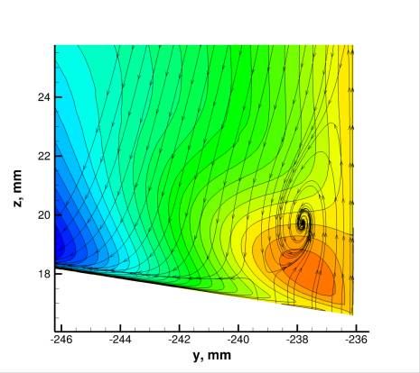
and the coefficients are: cb1 = 0.1355, σ = 2/3, cb2 = 0.622, κ = 0.41, cw1 = cκb12 + 1+c σ , cw2 = 0.3, cw3 = 2,
                                                                                                                                                                                                           b2

                                                                                                                cv1 = 7.1, ct3 = 1.2, and ct4 = 0.5. At viscous solid walls, the boundary condition is ν̂ = 0, and in the freestream
                                                                                                                ν̂ = 3.
                                                                                                                    The RC correction comes in solely through the fr1 term:
                                                                                                                                                                       2r∗ 
                                                                                                                                                                            1 − cr3 tan−1 (cr2 r̂) − cr1
                                                                                                                                                                                                  
                                                                                                                                                  fr1 = (1 + cr1 )        ∗
                                                                                                                                                                                                                                 (13)
                                                                                                                                                                      1+r
                                                                                                                where

                                                                                                                                                                          r∗ = S/ω                                               (14)
                                                                                                                                                                                                     
                                                                                                                                                       2ωik Sjk  DSij
                                                                                                                                                  r̂ =                + (εimn Sjn + εjmn Sin )Ω0m                                (15)
                                                                                                                                                         D4       Dt
Downloaded by NASA LANGLEY RESEARCH CENTRE on April 14, 2020 | http://arc.aiaa.org | DOI: 10.2514/6.2020-1304

                                                                                                                                                                                   
                                                                                                                                                                     1 ∂ui      ∂uj
                                                                                                                                                               Sij =         +                                                   (16)
                                                                                                                                                                     2 ∂xj      ∂xi
                                                                                                                                                                                         
                                                                                                                                                              1    ∂ui    ∂uj
                                                                                                                                                        ωij =          −        + 2εmji Ω0m                                      (17)
                                                                                                                                                              2    ∂xj    ∂xi

                                                                                                                                                                        S 2 = 2Sij Sij                                           (18)

                                                                                                                                                                        ω 2 = 2ωij ωij                                           (19)

                                                                                                                                                                      1 2
                                                                                                                                                                         S + ω2
                                                                                                                                                                      D2 =
                                                                                                                                                                                 
                                                                                                                                                                                                                          (20)
                                                                                                                                                                      2
                                                                                                                and Ω0m is zero for all computations in this paper. The constants are cr1 = 1.0, cr2 = 12, and cr3 = 1.0. The
                                                                                                                Lagrangian (material) derivative is:
                                                                                                                                                                  DSij   ∂Sij      ∂Sij
                                                                                                                                                                       ≡      + uk                                               (21)
                                                                                                                                                                   Dt     ∂t       ∂xk
                                                                                                                with the time term ignored for all of the computations in this paper, because they are solved as steady state.
                                                                                                                   As a linear eddy-viscosity model, SA-RC makes use of the Boussinesq assumption
                                                                                                                                                                                   
                                                                                                                                                                           1 ∂uk         2
                                                                                                                                                        τij = 2µt Sij −          δij − ρkδij                                     (22)
                                                                                                                                                                           3 ∂xk         3
                                                                                                                when determining the turbulent stress terms in the RANS equations, with the last term ignored for this model.

                                                                                                                2.   SA-RC-QCR2000
                                                                                                                The quadratic constitutive relation (QCR) methodology developed by Spalart [28] is an improvement over the Boussi-
                                                                                                                nesq relation. The turbulent stresses from SA-RC are modified via

                                                                                                                                                       τij,QCR = τij − Ccr1 [Oik τjk + Ojk τik ]                                 (23)
                                                                                                                where
                                                                                                                                                                                r
                                                                                                                                                                                ∂um ∂um
                                                                                                                                                              Oik = 2Wik /                                                       (24)
                                                                                                                                                                                ∂xn ∂xn
                                                                                                                                                                                      
                                                                                                                                                                          1 ∂ui    ∂uk
                                                                                                                                                                  Wik   =        −                                               (25)
                                                                                                                                                                          2 ∂xk    ∂xi
                                                                                                                and the constant is Ccr1 = 0.3.

                                                                                                                                                                             4 of 31
Reynolds-Averaged Navier-Stokes Computations of the NASA Juncture Flow Model Using FUN3D and OVERFLOW
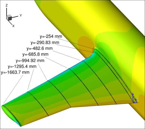
3.   SA-RC-QCR2013 and SA-RC-QCR2013-V
                                                                                                                In QCR2000, the 2ρkδij /3 term is still ignored in the implementation of τij into the RANS equations. Mani et
                                                                                                                al. [29] developed a QCR2013 version that includes an approximation to this term, which is not expected to have any
                                                                                                                significant effects at low Mach numbers such as those considered in this paper. The modification is:
                                                                                                                                                                                                      p
                                                                                                                                       τij,QCR2013 = τij − Ccr1 [Oik τjk + Ojk τik ] − Ccr2 µt              ∗ S∗ δ
                                                                                                                                                                                                          2Smn                     (26)
                                                                                                                                                                                                               mn ij

                                                                                                                with

                                                                                                                                                                 ∗             1 ∂uk
                                                                                                                                                                Sij = Sij −          δij                                           (27)
                                                                                                                                                                               3 ∂xk
                                                                                                                and Ccr2 = 2.5. However, some applications have noted numerical problems with the last term in Eq. (26), notably in
                                                                                                                wake regions where µt is not small. A recommended fix is to use vorticity instead of strain in this term. This form is
                                                                                                                referred to as QCR2013-V, as follows:
Downloaded by NASA LANGLEY RESEARCH CENTRE on April 14, 2020 | http://arc.aiaa.org | DOI: 10.2514/6.2020-1304

                                                                                                                                                                                              p
                                                                                                                                   τij,QCR2013−V = τij − Ccr1 [Oik τjk + Ojk τik ] − Ccr2 µt 2Wmn Wmn δij                         (28)
                                                                                                                For the applications in this paper, FUN3D was unable to run SA-RC-QCR2013 at all (because numerical issues caused
                                                                                                                the code to blow up). OVERFLOW was able to run SA-RC-QCR2013 in general, but it sometimes had difficulties
                                                                                                                with convergence. Both codes were able to run SA-RC-QCR2013-V without any problems.

                                                                                                                4.   Minor turbulence model variants: noft2
                                                                                                                A minor model variant for SA-RC, SA-RC-QCR2000, SA-RC-QCR2013, and SA-RC-QCR2013-V was employed
                                                                                                                by OVERFLOW. Termed “noft2”, this variant sets ft2 = 0 in the base SA model. Functionally, for fully-turbulent
                                                                                                                solutions at sufficiently high Reynolds numbers, there is no difference resulting from this change [19]. Throughout
                                                                                                                the paper, the “noft2” designation has been dropped.

                                                                                                                5.   Important consideration for normal turbulent stress output
                                                                                                                Recall that when using a linear model such as SA-RC, or when including the QCR2000 modification, the 2ρkδij /3
                                                                                                                term is typically ignored when forming τij in the RANS equations. This practice is considered acceptable because
                                                                                                                the normal stress magnitudes usually have very little influence on the mean flow in shear-flow-driven aerodynamic
                                                                                                                problems of interest (the normal stress differences have more of an impact). However, ignoring the term can be
                                                                                                                problematic for outputting and plotting the turbulent normal stresses (when comparing to experiment, for example).
                                                                                                                Therefore, in both FUN3D and OVERFLOW, when outputting the turbulent normal stresses for SA-RC or SA-RC-
                                                                                                                QCR2000, the term is approximately included via
                                                                                                                                                                                   p
                                                                                                                                                         2ρkδij /3 ≈ 2/3δij µt         2Sij Sij /a1                                (29)
                                                                                                                where a1 is taken as 0.31. This approximate relation came from Spalart and Allmaras [30], and this value for the
                                                                                                                “structure parameter” a1 is exactly the same used by Menter in his SST model [31]. This is similar to the approximation
                                                                                                                already included in QCR2013, except that the a1 constant in QCR2013 is 0.26667.

                                                                                                                D.     Grids
                                                                                                                The CFD grids are briefly described here.

                                                                                                                1.   Structured Overset
                                                                                                                A series of overset grids were created for the Juncture Flow Model. There is a commonality between the grids
                                                                                                                used in all of the CFD simulations. The grids were built using Chimera Grid Tools [32]. The full span JF model
                                                                                                                configuration consisted of a fuselage and two wings. The fuselage was built from 4 zones, two of which span the
                                                                                                                length of the fuselage, and two cap grids covering the nose and rear of the fuselage. The wing grids for all the various
                                                                                                                configurations shared a common 6 zone topology. The wing grids consisted of two collar grids covering the wing-
                                                                                                                fuselage junction, two grids spanning the wing, and two wing tip cap grids. Each pair of grids had overlap along
                                                                                                                the chord, making effectively a front and rear zone. All the surface grids were projected back to the reference CAD

                                                                                                                                                                         5 of 31
Reynolds-Averaged Navier-Stokes Computations of the NASA Juncture Flow Model Using FUN3D and OVERFLOW
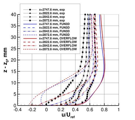
geometry using Pointwise R [33] to ensure a smooth surface geometry. For the free-air grids, a series of grids with
                                                                                                                increasing grid resolution were built. Four grid topologies, including a coarse, medium, fine, and extra-fine grid, were
                                                                                                                constructed. Figure 2 shows the grid density on the surface of the port wing and fuselage. The overall vehicle included
                                                                                                                16 grid zones, and Table 1 details the various configurations investigated in this study, and the grid metrics for each
                                                                                                                configuration. The near body grid point counts include just the volume grids for the JF model, excluding the support
                                                                                                                hardware, and applicable wind tunnel or off-body Cartesian grids.

                                                                                                                                                  Table 1. Summary of overset full-span structured grids.

                                                                                                                 Configuration                             Near Body Grid Points          Total Grid Points    Max Stretching Ratio
                                                                                                                 Free-Air Coarse (C)                                      19,370,462             21,374,458              1.20
                                                                                                                 Free-Air Medium (M)                                      48,942,491             50,917,459              1.15
                                                                                                                 Free-Air Fine (F)                                       171,553,707            173,206,274              1.10
Downloaded by NASA LANGLEY RESEARCH CENTRE on April 14, 2020 | http://arc.aiaa.org | DOI: 10.2514/6.2020-1304

                                                                                                                 Free-Air Extra Fine (XF)                                413,580,971            424,140,207              1.08
                                                                                                                 Wind Tunnel Medium (Tunnel M)                            48,942,491             94,572,947              1.15
                                                                                                                 Wind Tunnel Fine (Tunnel F)                             171,553,707            381,515,373              1.10

                                                                                                                    For the wind tunnel grids, wall grids were built from CAD based on the as-built laser scanned 14x22 as described
                                                                                                                in Nayani et al. [34]. Fifteen zones modeled the high-speed leg of the 14x22. The tunnel was split into five sections
                                                                                                                streamwise: plenum, test section, diffuser part 1, diffuser part 2, and extended diffuser. Each section was comprised
                                                                                                                of two viscous wall grids, and one core grid. The average grid spacing was varied to produce a medium (152.4 mm),
                                                                                                                and fine (76.2 mm) grid. Minimum spacing at the walls of the test section was less than 0.003048 mm on all grids.
                                                                                                                The straight section of the inlet, prior to the contraction, was run with inviscid walls. The diffuser grids gradually
                                                                                                                coarsened downstream. A diffuser extension of 30.48 m streamwise was incorporated, and the extended diffuser walls
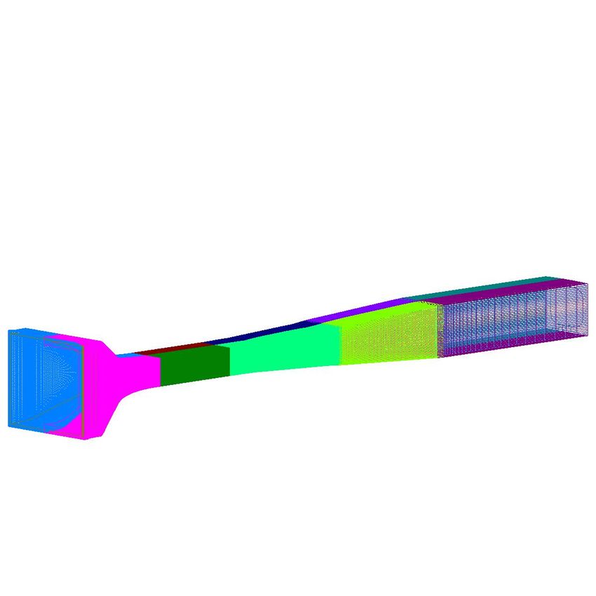
                                                                                                                also used an inviscid boundary condition. Figure 3 shows the wind tunnel volume grid with the extended diffuser, and
                                                                                                                an overall view of the 14x22 with the JF model installed. Utilizing inviscid sections of the tunnel helped increase the
                                                                                                                code stability, and helped accelerate the convergence of the CFD code. The details and benefits of using this method
                                                                                                                can be found in Lee et al. [14]. Domain connectivity and hole cutting was performed using OVERFLOW’s object
                                                                                                                xrays [35].
                                                                                                                    The JF model installation location for both α = 5.0◦ and α = −2.5◦ cases was based on laser scans in the test
                                                                                                                section. Different geometries were necessary for the two angles of attack, as the mast on the support changed to place
                                                                                                                the model in the center of the tunnel. Figure 4 shows a zoomed region of the test section with the JF model installed at
                                                                                                                both angles of incidence. For the wind tunnel results shown below, the free-air medium and fine grids were embedded
                                                                                                                directly into the wind tunnel configuration for consistency between free-air and tunnel calculations.
                                                                                                                    The wind tunnel with the JF model installed (at their respective angles of attack) were translated and rotated to
                                                                                                                match the same coordinate system as the free-air grid system (body coordinate system), to simplify the postprocessing.
                                                                                                                In doing this, all the flow quantities, velocities, etc. from a post processing standpoint, were already in the body
                                                                                                                coordinate system as opposed to the tunnel coordinate system. This eliminated the need to transform the flowfield data
                                                                                                                to the body coordinate system when postprocessing the data.

                                                                                                                2.   Unstructured
                                                                                                                In Rumsey et al. [16], a family of unstructured free-air half-span grids was utilized. The solutions were found to be
                                                                                                                highly grid-sensitive in and near the corner separation region. A second family of grids was subsequently created with
                                                                                                                a significantly higher degree of grid clustering in the corner region. Comparisons of predicted separation length and
                                                                                                                width for the particular case of α = 5◦ are shown in Fig. 5. The old and new M grids are compared in Figs. 5(a)
                                                                                                                and (b), respectively. Then, plots of separation length and width as a function of N −2/3 , where N represents the
                                                                                                                number of unknowns in the half-span grid, are shown in Figs. 5(c) and (d). For a code with second-order global spatial
                                                                                                                accuracy, the independent variable should vary linearly with N −2/3 on sufficiently refined grids. Results on both sets
                                                                                                                of grids approached the same result as the grid was refined (N −2/3 → 0). The new grids successfully produced less
                                                                                                                grid sensitivity and obtained more accurate results for a given grid size, compared with experiment (green square,
                                                                                                                including estimated uncertainty bars). However, as will be shown below, there was still a significant amount of grid
                                                                                                                sensitivity (changes in the solution with successively finer grids) in the separated region. This sensitivity underscores
                                                                                                                the fact that it is very difficult to attain so-called “grid convergence” for three-dimensional separated flows. The free-

                                                                                                                                                                          6 of 31
Reynolds-Averaged Navier-Stokes Computations of the NASA Juncture Flow Model Using FUN3D and OVERFLOW
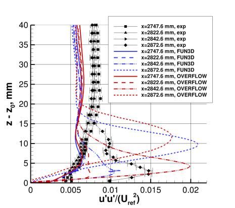
air half-span grids from Rumsey et al. [16] had the following approximate number of unknowns: 10.7, 35.7, 120.4, and
                                                                                                                258.4 million. The current unstructured grids, which were created using Pointwise R version 182.R2, are summarized
                                                                                                                in Table 2.

                                                                                                                                                Table 2. Summary of free-air half-span unstructured grids.

                                                                                                                        Grid                 Number of            Tets / Prisms /          Minimum wall      Stretching rate
                                                                                                                                            unknowns (N)        Pyramids (millions)        spacing (mm)         near wall
                                                                                                                        Coarse (C)               12,312,544            10 / 21 / 0.07           0.00135            1.25
                                                                                                                        Medium (M)               39,121,991            20 / 71 / 0.15           0.00090            1.16
                                                                                                                        Fine (F)                160,761,294          223 / 245 / 0.41           0.00060            1.10
                                                                                                                        Extra Fine (XF)         356,610,207          356 / 591 / 0.85           0.00040            1.07
Downloaded by NASA LANGLEY RESEARCH CENTRE on April 14, 2020 | http://arc.aiaa.org | DOI: 10.2514/6.2020-1304

                                                                                                                    A few FUN3D runs were also made of the model (full span) in the 14x22, including the mast and sting support
                                                                                                                system. In these cases, the M grid near the model was used as a starting point, then it was extended to model the
                                                                                                                high-speed leg of the wind tunnel. The wind tunnel’s contraction and diffuser sections were both included. To avoid
                                                                                                                problems with separated flow near the outflow, a constant-area extension was added downstream of the diffuser, similar
                                                                                                                to OVERFLOW’s tunnel grids. For the FUN3D cases, the wind tunnel walls were treated as inviscid surfaces. The total
                                                                                                                number of unknowns for the tunnel grids was around 80 million for both the cases of 5◦ and −2.5◦ angle of incidence.
                                                                                                                Like OVERFLOW, FUN3D translated and rotated the tunnel system to match the free-air system, for postprocessing
                                                                                                                convenience.

                                                                                                                E.   Flow Conditions
                                                                                                                In the 14x22, the Reynolds number (based on the crank chord length) was held fixed at 2.4 million (±0.3%) throughout
                                                                                                                the testing. However, the atmospheric conditions varied, so that the Mach number ranged from about 0.175 to 0.205,
                                                                                                                temperature ranged from about 275 to 308 K, and dynamic pressure ranged from about 2107 to 2921 Pa. In this study,
                                                                                                                the median values from the test of M = 0.189 and T = 288.84 K were used. The median dynamic pressure was
                                                                                                                approximately 2476 Pa.
                                                                                                                    Two angles of incidence were selected in the experiment for detailed data collection: nominally 5◦ and −2.5◦ .
                                                                                                                These choices yielded two different separation sizes (larger and smaller, respectively). The actual ranges throughout
                                                                                                                the testing were approximately 4.97◦ < α < 5.04◦ and −2.54◦ < α < −2.48◦ . For this CFD study, the nominal
                                                                                                                uncorrected angles of α = 5◦ and −2.5◦ were employed for the free-air computations. Because of wind tunnel wall
                                                                                                                influence, the angles of attack used for free-air computations should include some correction. However, there was no
                                                                                                                accurate estimate of the corrections required because no balance data were collected in this experiment. In this paper,
                                                                                                                results are also shown for computations that include the wind tunnel walls, for which no angle-of-attack correction is
                                                                                                                needed, and an assessment is made regarding the walls’ impact on the juncture flow region quantities of interest.

                                                                                                                                                                    III.     Results
                                                                                                                     The CFD results and comparisons with experiment are described in this section. For FUN3D, the mean flow and
                                                                                                                turbulence model residuals typically converged iteratively at least 6 orders of magnitude, yielding steady-state RANS
                                                                                                                results. However, on the XF grid, the FUN3D residuals hung up after converging only a few orders. Nonetheless,
                                                                                                                these XF solutions appeared to be consistent with what was expected based on the coarser grid solutions, so they are
                                                                                                                still included here. The 5◦ tunnel run converged well, but at −2.5◦ convergence was poor, likely due to localized
                                                                                                                shedding from the extended mast. For OVERFLOW, the mean flow residuals typically converged around 6 orders
                                                                                                                of magnitude, and the turbulence residuals converged around 4 orders of magnitude. The residuals for the wind
                                                                                                                tunnel cases were prevented from converging because the support hardware (particularly the mast) exhibited localized
                                                                                                                shedding. Although no balance data were taken in this experiment, CFD produced lift and drag coefficient values
                                                                                                                roughly in the range of CL ≈ 0.85 − 0.86, CD ≈ 0.067 − 0.070 for 5◦ , and CL ≈ 0.20 − 0.21, CD ≈ 0.027 − 0.029
                                                                                                                for −2.5◦ . The reference area was taken to be 965543.23 mm2 for the semi-span model.

                                                                                                                                                                           7 of 31
Reynolds-Averaged Navier-Stokes Computations of the NASA Juncture Flow Model Using FUN3D and OVERFLOW
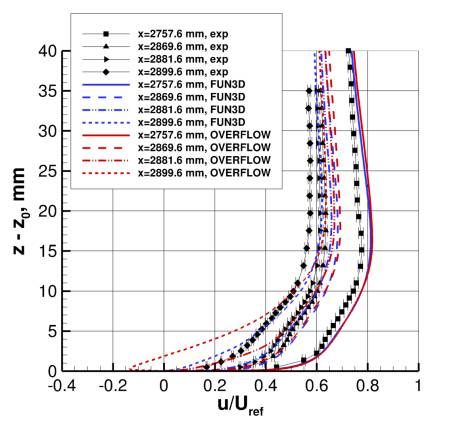
A.   Surface Flow Separation Predictions
                                                                                                                Figure 6 shows surface-restricted streamlines from FUN3D free-air computations at α = 5◦ on the finest three grids
                                                                                                                using the SA-RC-QCR2013-V turbulence model. The predicted separation size decreased with grid size, with more
                                                                                                                changes evident between M and F than between F and XF. Although not shown, surface-restricted streamlines from
                                                                                                                OVERFLOW indicated similar results.
                                                                                                                    Comparisons between CFD and experiment separation sizes are shown in Fig. 7. Here, even though OVERFLOW
                                                                                                                ran on full-span grids, its results are plotted as a function of its half-span grid size, for direct comparison with FUN3D.
                                                                                                                Qualitatively, the SA-RC model produced a separation that was too long by around 100 percent. FUN3D results were
                                                                                                                steady, but OVERFLOW results with SA-RC exhibited unsteadiness in the separation regions when using the C and
                                                                                                                M grids, with variations of as much as 20 mm in length or width for steady-state runs. Changing to time-accurate runs
                                                                                                                did not make much difference. Here, an attempt was made to plot OVERFLOW’s average values, which can therefore
                                                                                                                be considered only approximate. Because the SA-RC model produced a separation that was clearly much too large, it
                                                                                                                is not considered a viable choice for predicting this type of flow. Therefore, in the interest of space, detailed SA-RC
                                                                                                                results will not be shown in the remaining sections of this paper, with one exception.
Downloaded by NASA LANGLEY RESEARCH CENTRE on April 14, 2020 | http://arc.aiaa.org | DOI: 10.2514/6.2020-1304

                                                                                                                    The QCR corrections improved the predictions significantly. Results for SA-RC-QCR2000, SA-RC-QCR2013,
                                                                                                                and SA-RC-QCR2013-V were nearly the same, as expected for this low Mach number flow. In fact, in FUN3D,
                                                                                                                results between SA-RC-QCR2000 and SA-RC-QCR2013-V were nearly indistinguishable. Results from FUN3D and
                                                                                                                OVERFLOW were not identical, but were fairly close overall. As the grid was refined, the QCR-based models in both
                                                                                                                codes predicted about the correct separation width compared with experiment, but predicted a length that was still
                                                                                                                somewhat too high; i.e., the corner separation started too far upstream on the wing.

                                                                                                                B.   Surface Pressure Predictions
                                                                                                                Surface pressure coefficient comparisons on the wing are shown in Figs. 8 and 9 for SA-RC-QCR2013-V. For brevity,
                                                                                                                only surface pressures at α = 5◦ are shown; results at α = −2.5◦ do not add any additional insights. (The interested
                                                                                                                reader can refer to earlier publications [16,17] for other results.) In these figures, experimental data from multiple runs
                                                                                                                on both left and right wings are plotted; thus, the data scatter provide a feel for the uncertainty in the measurements.
                                                                                                                    At most wing sections, both FUN3D and OVERFLOW yielded approximately the same results, and there were
                                                                                                                insignificant differences between grids. However, at the station y = −1663.7 mm near the wing tip, there was a large
                                                                                                                influence of the grid, presumably because of a need to resolve the tip vortex. Here, the unstructured M grid was clearly
                                                                                                                too coarse. Differences were evident between the two codes on the F and XF grids at this station, but the two finest
                                                                                                                overset grids appeared to be sufficiently resolved in OVERFLOW. At the innermost span station of y = −254 mm,
                                                                                                                which cuts through the separation at this angle of attack, there were differences due to both grid and code near the
                                                                                                                wing trailing edge (see the inset in Fig. 8(b)). These differences highlight the difficulty inherent in attaining grid- and
                                                                                                                code-converged results in separation regions of three-dimensional configurations.
                                                                                                                    At y = −254 mm, there was significant disagreement at one data point near the leading edge suction peak between
                                                                                                                CFD and experiment. It is not clear at this time whether this discrepancy was due to CFD inadequacy or if there was
                                                                                                                a problem with that particular pressure port. This question will be addressed in a follow-up experiment.

                                                                                                                C.   Flowfield Predictions
                                                                                                                Next we turn to comparisons of flowfield quantities: velocity and turbulent Reynolds stress profiles, measured ex-
                                                                                                                perimentally using LDV and including estimated uncertainty (error bars). The main focus here is on the SA-RC-
                                                                                                                QCR2013-V turbulence model at α = 5◦ . As mentioned earlier, the other QCR variants yielded essentially the same
                                                                                                                mean flow results, so their results will not be shown here.
                                                                                                                    Figure 10 shows results far upstream on the side of the fuselage (see Fig. 10(a)). At this location, the flow was
                                                                                                                attached and well behaved, and most RANS models would be expected to predict the mean flow here well. Indeed,
                                                                                                                as shown in Fig. 10(b), the three velocity components agreed well with experiment, although the CFD u-profile
                                                                                                                appeared to show a somewhat thicker boundary layer than experiment. The turbulent normal stresses, shown in
                                                                                                                Fig. 10(c), indicated some disagreement between CFD and experiment, especially in the u0 u0 component near the
                                                                                                                wall. The turbulent shear stresses u0 v 0 and v 0 w0 agreed fairly well with experiment, whereas u0 w0 was slightly off
                                                                                                                (Fig. 10(d)). In all cases, there was very little difference between results on the M, F, or XF grids, and both FUN3D
                                                                                                                and OVERFLOW produced essentially identical results. This agreement indicates that the finer grids were fine enough
                                                                                                                to attain essentially “grid-converged” results in this region of the flowfield, and the respective implementations of the
                                                                                                                SA-RC-QCR2013-V model in FUN3D and OVERFLOW were consistent.

                                                                                                                                                                          8 of 31
Reynolds-Averaged Navier-Stokes Computations of the NASA Juncture Flow Model Using FUN3D and OVERFLOW
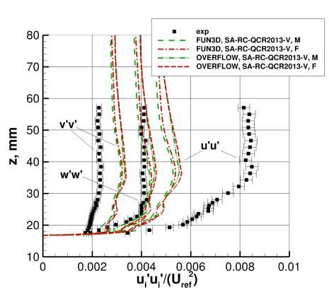
A similar set of results is shown on the wing, in the corner well upstream of separation, in Fig. 11. At this location
                                                                                                                (x = 2747.6 mm, y = −237.1 mm), the influence of grid and CFD code was now visible, but was generally very
                                                                                                                small, indicating sufficient grid density for capturing the flow in this attached-flow region. At this location, both CFD
                                                                                                                codes yielded consistent results. Compared to experiment, the u-velocity component was overpredicted in magnitude,
                                                                                                                although the inflection in the profile was seen. The w0 w0 component of Reynolds stress was predicted well, but v 0 v 0
                                                                                                                was somewhat overpredicted and u0 u0 was significantly underpredicted. This latter underprediction occurred because
                                                                                                                this profile was located only 1 mm from the fuselage, well within the fuselage boundary layer, and as the earlier results
                                                                                                                on the fuselage showed, this turbulence model underpredicts u0 u0 near the wall. The u0 v 0 and v 0 w0 components were
                                                                                                                again predicted extremely well compared with experiment, whereas the u0 w0 component was off.
                                                                                                                    Further downstream, near the start of the separation, profiles are shown outboard of the fuselage boundary layer
                                                                                                                (and outboard of the start of separation) in Fig. 12. Here, both codes produced consistent results, and there was little
                                                                                                                influence due to grid size. Computed velocity profiles agreed generally well with experiment, but Reynolds stresses
                                                                                                                showed some differences, particularly in u0 u0 and u0 w0 .
                                                                                                                    Figure 13 shows results very near the fuselage, near the start of separation. Here, at x = 2852.6 mm, y =
Downloaded by NASA LANGLEY RESEARCH CENTRE on April 14, 2020 | http://arc.aiaa.org | DOI: 10.2514/6.2020-1304

                                                                                                                −237.1 mm, the CFD results showed a significant amount of separation as well as noticeable grid sensitivity (the CFD
                                                                                                                separation point was well upstream). The experiment was believed to have separated just prior to this location; clearly
                                                                                                                the size of its separated flow region was smaller than that predicted by CFD. This location also shows larger differences
                                                                                                                between FUN3D and OVERFLOW. In particular, the FUN3D results on the M grid appeared to be significantly
                                                                                                                underresolved. At this location, as well as further downstream into the separation region (not shown), the CFD ceased
                                                                                                                to correlate with the experiment.
                                                                                                                    In Figs. 14 and 15, the progression of profiles moving along the x-direction is shown 3 mm from the fuselage,
                                                                                                                for the α = 5◦ case. Figure 14(a) shows the four locations. In these figures, z0 , the location of the wing surface,
                                                                                                                has been subtracted from z on the y-axis of the plots to make comparisons easier. In Figs. 14(b)-(d), the velocity
                                                                                                                components indicated too large a magnitude upstream in the CFD, then early separation compared with experiment.
                                                                                                                The two codes (only XF results from each is shown here) agreed well with each other upstream of separation, but then
                                                                                                                showed significant differences in and near separation. Reynolds stress profiles, shown in Figs. 15(a)-(f), showed that a
                                                                                                                large change took place in the experiment between stations x = 2842.6 mm and x = 2872.6 mm, whereas in the CFD
                                                                                                                the change took place upstream of this. Because of the misprediction of separation location in the CFD and because of
                                                                                                                the grid sensitivity of the CFD in and near separation, it is difficult to make comparisons and draw conclusions from
                                                                                                                downstream profiles.
                                                                                                                    Finally, a progression of profile results is shown at α = −2.5◦ in Figs. 16 and 17. In this case, the SA-RC-
                                                                                                                QCR2013-V results agreed somewhat better with experiment upstream of separation than it did for α = 5◦ , but then
                                                                                                                separation was again predicted somewhat too far upstream. In terms of Reynolds stresses, the experiment generally
                                                                                                                showed very little differences at the four selected stations, whereas CFD indicated larger variations downstream,
                                                                                                                because of its earlier separation prediction. The two CFD codes on their respective XF grids agreed well upstream of
                                                                                                                separation, but then (again) deviated once separation had taken place.
                                                                                                                    It is believed that the differences between the turbulent normal stresses are a driver for near-wall secondary corner
                                                                                                                vortical flow, which, when present, acts to inhibit corner separation [2]. Linear models like SA-RC provide no differ-
                                                                                                                ences between the normal stresses, and hence do not provide sufficient vorticity for suppressing the corner separation.
                                                                                                                An example is shown in Fig. 18. In Fig. 18(a), the turbulent normal stresses are shown at the location x = 2747.6
                                                                                                                mm, y = −237.1 mm from the SA-RC model. Figure 18(b) shows results using the SA-RC-QCR2013-V model (also
                                                                                                                shown earlier in Fig. 11(c)). It is clear that without the QCR correction, the SA-RC model produced turbulent normal
                                                                                                                stresses with virtually no difference between them, as expected. The QCR correction separated the normal stresses
                                                                                                                to some degree. (Although not shown, the QCR correction only had relatively small influence on the turbulent shear
                                                                                                                stresses.) Figures 18(c) and (d) show contours of v velocity in the plane x = 2747.6 mm, with in-plane streamtraces
                                                                                                                superimposed using (v, w+0.11) (the addition of 0.11 is done to approximately remove the bulk downward velocity
                                                                                                                at this location as the flow follows the wing). These streamtraces demonstrate that the SA-RC-QCR2013-V model
                                                                                                                yielded some vortical behavior near the junction, whereas the SA-RC model did not. Figures 18(e) and (f) empha-
                                                                                                                size the difference by superimposing a three-dimensional isosurface of Q-criterion (second invariant of ∇u). This
                                                                                                                isosurface highlights the vortical flow present near the juncture corner when QCR is employed.
                                                                                                                    The QCR correction improved the comparison with experiment in terms of both the turbulent normal stresses
                                                                                                                and the resulting separation size, but greater differences between the normal stresses existed in the experiment. The
                                                                                                                fact that the current QCR correction underpredicted these levels may be the reason why the separation size was still
                                                                                                                somewhat too large compared with experiment.

                                                                                                                                                                          9 of 31
Reynolds-Averaged Navier-Stokes Computations of the NASA Juncture Flow Model Using FUN3D and OVERFLOW
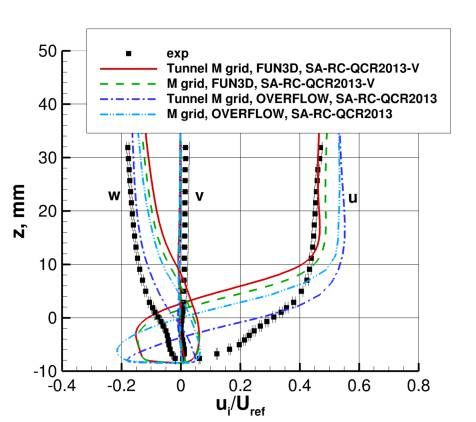
D.   Effect of Wind Tunnel Walls
                                                                                                                A number of CFD runs have been made with the model in the 14x22, especially with OVERFLOW. See, for example,
                                                                                                                Lee and Pulliam [17] for details. Here, only a brief summary of the tunnel wall influence is provided. Generally
                                                                                                                speaking, including the tunnel walls does have some effect, but it is relatively insignificant in terms of the general
                                                                                                                character of the CFD predictions in the juncture flow region itself.
                                                                                                                    Figure 19 shows the separation size predicted by including wind tunnel walls in the computations. To enable direct
                                                                                                                comparison with the free-air results, the N for the tunnel results is represented by its near-body half-grid size. For
                                                                                                                FUN3D (only computed on one grid based on the free-air M size), which treated the tunnel walls inviscidly, including
                                                                                                                the walls yielded a slightly larger separation. For OVERFLOW, which treated the tunnel walls (mostly) as viscous,
                                                                                                                solid boundaries, the separation size slightly decreased. The reason for the opposite trends with the two codes is not
                                                                                                                known. It seems unlikely that the different treatment of the wall boundary condition would have a significant influence.
                                                                                                                It may be only that the trends were different on the grid levels examined, but would become consistent on more refined
                                                                                                                grids. In any case, the effect of tunnel walls was relatively small. We turn next to the flowfield details.
                                                                                                                    Figures 20, 21, and 22 show the tunnel M grid results from FUN3D and OVERFLOW compared with corre-
Downloaded by NASA LANGLEY RESEARCH CENTRE on April 14, 2020 | http://arc.aiaa.org | DOI: 10.2514/6.2020-1304

                                                                                                                sponding free-air M grid results. Here, FUN3D used SA-RC-QCR2013-V and OVERFLOW used SA-RC-QCR2013.
                                                                                                                Outside of the separated flow region (Figs. 20 and 21), all CFD results were very close for the mean flow and turbu-
                                                                                                                lence quantities. Inside of the separation region (Fig. 22), there were significant differences between the computations,
                                                                                                                but no particular trends due to wind tunnel walls were evident. Differences between CFD and experiment tended to be
                                                                                                                more significant than differences between the CFD runs with and without wind tunnel walls.

                                                                                                                                                                 IV.   Conclusions
                                                                                                                    The two CFD codes FUN3D and OVERFLOW have played a significant role throughout the life of the NASA
                                                                                                                Juncture Flow project. They were used to help design the experiment in conjunction with risk-reduction testing. Now
                                                                                                                that the initial phase of the experiment has been completed, evaluation of turbulence model capabilities for predicting
                                                                                                                this particular type of separated flow has begun. In this paper, the abilities of the Spalart-Allmaras class of RANS
                                                                                                                turbulence model were summarized.
                                                                                                                    Generally, both FUN3D and OVERFLOW produced consistent predictions of separation size when using the same
                                                                                                                turbulence model. In terms of velocity and Reynolds stress details, the codes were consistent in attached flow regions.
                                                                                                                Predicted velocities in these regions agreed fairly well with experiment, but Reynolds stresses were sometimes in
                                                                                                                agreement and sometimes not, with the greatest errors tending to be in the normal components. The flow in the
                                                                                                                separated juncture flow region was found to be highly sensitive to the grid employed, and not in good agreement with
                                                                                                                experiment. Even on the finest grids in this study (on the order of 400 million unknowns), results in the separation
                                                                                                                area still exhibited grid sensitivity. This sensitivity highlights the known difficulty achieving grid convergence for
                                                                                                                three-dimensional separated flows. In spite of the grid sensitivity, some general conclusions regarding the capabilities
                                                                                                                of the RANS turbulence models for this separated flow could still be made.
                                                                                                                    The impact of including wind tunnel walls on the prediction of details in the juncture flow region was found to be
                                                                                                                relatively minor. In other words, conclusions regarding efficacy of the RANS turbulence models could be made for this
                                                                                                                case by using free-air computations. The confidence in these conclusions is particularly high because of the extensive
                                                                                                                grid studies included and the comparisons made between the two different CFD codes. The SA-RC model predicted
                                                                                                                separation size to be about two times too long compared to experiment. Different versions of a quadratic constitutive
                                                                                                                relation (QCR) were described, including a new version of QCR2013 (termed QCR2013-V) that was more robust.
                                                                                                                All versions of QCR, when used in conjunction with SA-RC, yielded consistent results with significantly improved
                                                                                                                separation predictions compared to SA-RC alone. However, although the QCR variants yielded approximately the
                                                                                                                correct separation width on refined grids, the separation length was still somewhat too long. The reason why the QCR
                                                                                                                methodology reduced separation size was primarily attributed to its better prediction of the differences between the
                                                                                                                turbulent normal stresses, which induced secondary corner vortical flow that acted to delay separation onset. Although
                                                                                                                improved with QCR, these differences between the normal stresses were still less than in the experiment, particularly
                                                                                                                because of underprediction of the u0 u0 component very near both walls. This leads to the hypothesis that further minor
                                                                                                                modifications to QCR that improve predictions of the turbulent normal stresses could lead to even more accurate
                                                                                                                predictions of the corner separation size.

                                                                                                                                                                         10 of 31
Acknowledgments
                                                                                                                    The authors gratefully acknowledge other active members of the JF Team. From NASA, this includes Mike
                                                                                                                Kegerise, Dan Neuhart, Judi Hannon, Luther Jenkins, Jan Carlson, Nashat Ahmad, Cathy McGinley, Scott Bartram,
                                                                                                                C.-S. Yao, Mujeeb Malik, P. Balakumar, Joe Morrison, and James Bell. The authors also acknowledge Philippe Spalart,
                                                                                                                Bill Oberkampf, Roger Simpson, and Gwibo Byun for their significant contributions. This work was supported by
                                                                                                                NASA’s Transformational Tools and Technologies (TTT) project of the Transformative Aeronautics Concepts Pro-
                                                                                                                gram.

                                                                                                                                                                                References
                                                                                                                      1 Gand, F., Deck, S., and Brunet, V., “Flow Dynamics Past a Simplified Wing Body Junction,” Physics of Fluids, Vol. 22, No. 11, 2010,

                                                                                                                pp. 11511, doi: https://doi.org/10.1063/1.3500697.
                                                                                                                      2 Bordji, M., Gand, F., Deck, S., and Brunet, V., “Investigation of a Nonlinear Reynolds-Averaged Navier-Stokes Closure for Corner Flows,”

                                                                                                                AIAA Journal, Vol. 54, No. 2, 2016, pp. 386–398, doi: https://doi.org/10.2514/1.J054313.
Downloaded by NASA LANGLEY RESEARCH CENTRE on April 14, 2020 | http://arc.aiaa.org | DOI: 10.2514/6.2020-1304

                                                                                                                      3 Wood, D. H. and Westphal, R. V., “Measurements of the Flow Around a Lifting-Wing/Body Junction,” AIAA Journal, Vol. 30, No. 1, 1992,

                                                                                                                pp. 6–12, doi: https://doi.org/10.2514/3.10875.
                                                                                                                      4 Simpson, R. L., “Juncture Flows,” Annual Review of Fluid Mechanics, Vol. 33, 2001, pp. 415–443, doi: https://doi.org/10.1146/

                                                                                                                annurev.fluid.33.1.415.
                                                                                                                      5 Gand, F., Brunet, V., and Deck, S., “A Combined Experimental, RANS and LES Investigation of a Wing Body Junction Flow,” AIAA Paper

                                                                                                                2010-4753, June-July 2010, doi: https://doi.org/10.2514/6.2010-4753.
                                                                                                                      6 Gand, F., Brunet, V., and Deck, S., “Experimental and Numerical Investigation of a Wing Body Junction Flow,” AIAA Journal, Vol. 50,

                                                                                                                No. 12, 2012, pp. 2711–2719, doi: https://doi.org/10.2514/1.J051462.
                                                                                                                      7 Gand, F., Monnier, J.-C., Deluc, J.-M., and Choffat, A., “Experimental Study of the Corner Flow Separation on a Simplified Junction,” AIAA

                                                                                                                Journal, Vol. 53, No. 10, 2015, pp. 2869–2877, doi: https://doi.org/10.2514/1.J053771.
                                                                                                                      8 Rumsey, C., Neuhart, D., and Kegerise, M., “The NASA Juncture Flow Experiment: Goals, Progress, and Preliminary Testing,” AIAA Paper

                                                                                                                2016–1557, January 2016, doi: https://doi.org/10.2514/6.2016-1557.
                                                                                                                      9 Kuester, M. S., Borgoltz, A., and Devenport, W., “Experimental Visualization of Junction Separation Bubbles at Low- to Moderate-Reynolds

                                                                                                                Numbers,” AIAA Paper 2016–3880, June 2016, doi: https://doi.org/10.2514/6.2016-3880.
                                                                                                                     10 Rumsey, C. and Morrison, J. H., “Goals and Status of the NASA Juncture Flow Experiment,” No. STO-MP-AVT-246-03, NATO Science

                                                                                                                and Technology Organization, AVT-246 Specialists Meeting on Progress and Challenges in Validation Testing for Computational Fluid Dynamics,
                                                                                                                Avila, Spain, 2016.
                                                                                                                     11 Kegerise, M. A. and Neuhart, D. H., “Wind Tunnel Test of a Risk-Reduction Wing/Fuselage Model to Examine Juncture-Flow Phenomena,”

                                                                                                                NASA TM–219348, November 2016, https://ntrs.nasa.gov/archive/nasa/casi.ntrs.nasa.gov/20160014854.pdf.
                                                                                                                     12 Lee, H. C., Pulliam, T. H., Neuhart, D., and Kegerise, M. A., “CFD Analysis in Advance of the NASA Juncture Flow Experiment,” AIAA

                                                                                                                Paper 2017-4127, 2017, doi: https://doi.org/10.2514/6.2017-4127.
                                                                                                                     13 Rumsey, C. L., Carlson, J. R., Hannon, J. A., Jenkins, L. N., Bartram, S. M., Pulliam, T. H., and Lee, H. C., “Boundary Condition

                                                                                                                Study for the Juncture Flow Experiment in the NASA Langley 14x22-Foot Subsonic Wind Tunnel,” AIAA Paper 2017-4126, June 2017, doi:
                                                                                                                https://doi.org/10.2514/6.2017-4126.
                                                                                                                     14 Lee, H. C., Pulliam, T. H., Rumsey, C. L., and Carlson, J. R., “Simulations of the NASA Langley 14- by 22-Foot Subsonic Tunnel for

                                                                                                                the Juncture Flow Experiment,” No. STO-MP-AVT-284-02, NATO Science and Technology Organization, AVT-284 Workshop on Advanced Wind
                                                                                                                Tunnel Boundary Simulation, Torino, Italy, 2018.
                                                                                                                     15 Rumsey, C. L., “The NASA Juncture Flow Test as a Model for Effective CFD/Experimental Collaboration,” AIAA Paper 2018-3319, June

                                                                                                                2018, doi: https://doi.org/10.2514/6.2018-3319.
                                                                                                                     16 Rumsey, C. L., Carlson, J.-R., and Ahmad, N., “FUN3D Juncture Flow Computations Compared with Experimental Data,” AIAA Paper

                                                                                                                2019-0079, January 2019, doi: https://doi.org/10.2514/6.2019-0079.
                                                                                                                     17 Lee, H. C. and Pulliam, T. H., “Overflow Juncture Flow Computations Compared with Experimental Data,” AIAA Paper 2019-0080, January

                                                                                                                2019, doi: https://doi.org/10.2514/6.2019-0080.
                                                                                                                     18 Kegerise, M. A. and Neuhart, D. H., “An Experimental Investigation of a Wing-Fuselage Junction Model in the NASA Langley 14- by

                                                                                                                22-Foot Subsonic Tunnel,” NASA TM–2019-220286, June 2019, https://ntrs.nasa.gov/archive/nasa/casi.ntrs.nasa.gov/
                                                                                                                20190027403.pdf.
                                                                                                                     19 Rumsey, C. L., “NASA Langley Research Center Turbulence Modeling Resource,” https://turbmodels.larc.nasa.gov, Ac-

                                                                                                                cessed: 2019-10-11.
                                                                                                                     20 “FUN3D User’s Manual,” https://fun3d.larc.nasa.gov, Accessed: 2019-10-11.
                                                                                                                     21 Nichols, R. H. and Buning, P. G., “User’s Manual for Overflow 2.2,” https://overflow.larc.nasa.gov/home/

                                                                                                                users-manual-for-overflow-2-2/, Accessed: 2019-10-11.
                                                                                                                     22 Spalart, P. R. and Allmaras, S. R., “A One-Equation Turbulence Model for Aerodynamic Flows,” Recherche Aerospatiale, Vol. 1, 1994,

                                                                                                                pp. 5–21.
                                                                                                                     23 Anderson, W. and Bonhaus, D., “An Implicit Upwind Algorithm for Computing Turbulent Flows on Unstructured Grids,” Computers and

                                                                                                                Fluids, Vol. 23, No. 1, 1994, pp. 1–22, doi: https://doi.org/10.1016/0045-7930(94)90023-X.
                                                                                                                     24 Anderson, W., Rausch, R., and Bonhaus, D. L., “Implicit/Multigrid Algorithms for Incompressible Turbulent Flows on Unstructured Grids,”

                                                                                                                Journal of Computational Physics, Vol. 128, 1996, pp. 391–408, doi: https://doi.org/10.1006/jcph.1996.0219.
                                                                                                                     25 Roe, P. L., “Approximate Riemann Solvers, Parameter Vectors, and Difference Schemes,” Journal of Computational Physics, Vol. 43, 1981,

                                                                                                                pp. 357–372, doi: https://doi.org/10.1016/0021-9991(81)90128-5.

                                                                                                                                                                                    11 of 31
26 Carlson, J., “Automated Boundary Conditions for Wind Tunnel Simulations,” NASA TM 2018-219812, March 2018, https://ntrs.

                                                                                                                nasa.gov/archive/nasa/casi.ntrs.nasa.gov/20180002095.pdf.
                                                                                                                     27 Shur, M. L., Strelets, M. K., Travin, A. K., and Spalart, P. R., “Turbulence Modeling in Rotating and Curved Channels: Assessing the

                                                                                                                Spalart-Shur Correction,” AIAA Journal, Vol. 38, No. 5, 2000, pp. 784–792, doi: https://doi.org/10.2514/2.1058.
                                                                                                                     28 Spalart, P. R., “Strategies for Turbulence Modelling and Simulation,” International Journal of Heat and Fluid Flow, Vol. 21, 2000, pp. 252–

                                                                                                                263, doi: https://doi.org/10.1016/S0142-727X(00)00007-2.
                                                                                                                     29 Mani, M., Babcock, D., Winkler, C., and Spalart, P., “Predictions of a Supersonic Turbulent Flow in a Square Duct,” AIAA Paper 2013–0860,

                                                                                                                January 2013, doi: https://doi.org/10.2514/6.2013-0860.
                                                                                                                     30 Spalart, P. R. and Allmaras, S. R., “A One-Equation Turbulence Model for Aerodynamic Flows,” AIAA Paper 1992–0439, January 1992,

                                                                                                                doi: https://doi.org/10.2514/6.1992-439.
                                                                                                                     31 Menter, F. R., “Two-Equation Eddy-Viscosity Turbulence Models for Engineering Applications,” AIAA Journal, Vol. 32, No. 8, 1994,

                                                                                                                pp. 1598–1605, doi: https://doi.org/10.2514/3.12149.
                                                                                                                     32 Chan, W. M., Gomez, R. J., Rogers, S. E., and Buning, P. G., “Best Practices in Overset Grid Generation,” AIAA Paper 2002-3191, June

                                                                                                                2002, doi: https://doi.org/10.2514/6.2002-3191.
                                                                                                                     33 “User’s Manual, Pointwise V18,” https://www.pointwise.com/doc/user-manual/, Accessed: 2019-10-11.
                                                                                                                     34 Nayani, S. N., Sellers, W., Brynildsen, S. E., and Everhart, J. L., “Numerical Study of the High-Speed Leg of a Wind Tunnel,” AIAA Paper

                                                                                                                2015–2022, January 2015, doi: https://doi.org/10.2514/6.2015-2022.
Downloaded by NASA LANGLEY RESEARCH CENTRE on April 14, 2020 | http://arc.aiaa.org | DOI: 10.2514/6.2020-1304

                                                                                                                     35 Meakin, R. L., “Object X-Rays for Cutting Holes in Composite Overset Structured Grids,” AIAA Paper 2001–2537, June 2001, doi: https:

                                                                                                                //doi.org/10.2514/6.2001-2537.

                                                                                                                Figure 1. The NASA Juncture Flow model, with inset showing an oil flow photograph of the upper surface wing junction separation at 5◦
                                                                                                                angle of incidence.

                                                                                                                                                                                     12 of 31
Downloaded by NASA LANGLEY RESEARCH CENTRE on April 14, 2020 | http://arc.aiaa.org | DOI: 10.2514/6.2020-1304

                                                                       (c) Fine
                                                                                                                                                (a) Coarse

13 of 31
           Figure 2. Comparison of overset surface grid resolutions.
                                                                                                                                                (b) Medium

                                                                       (d) Extra Fine
Downloaded by NASA LANGLEY RESEARCH CENTRE on April 14, 2020 | http://arc.aiaa.org | DOI: 10.2514/6.2020-1304

                                                                                                                                                 (a) Volume grid

                                                                                                                                      (b) Juncture Flow model grid installed

                                                                                                                       Figure 3. 14x22 wind tunnel, high-speed leg with extended diffuser.

                                                                                                                (a) α = 5.0◦                                                       (b) α = −2.5◦

                                                                                                                      Figure 4. Juncture Flow model as installed in the 14x22 wind tunnel.

                                                                                                                                                    14 of 31
Downloaded by NASA LANGLEY RESEARCH CENTRE on April 14, 2020 | http://arc.aiaa.org | DOI: 10.2514/6.2020-1304

                                                                                                                (a) Surface grid resolution of medium grid from AIAA-2019-0079            (b) Surface grid resolution of current medium grid

                                                                                                                           (c) Separation length predictions, α = 5◦                          (d) Separation width predictions, α = 5◦

                                                                                                                                    Figure 5. Comparison of results on different set of unstructured grids, SA-RC-QCR2013-V.

                                                                                                                                                                             15 of 31
(a) Medium grid                                (b) Fine grid                               (c) Extra-fine grid

                                                                                                                Figure 6. Computed surface streamlines from FUN3D, SA-RC-QCR2013-V, colored by cf,x (α = 5◦ free-air computation).
Downloaded by NASA LANGLEY RESEARCH CENTRE on April 14, 2020 | http://arc.aiaa.org | DOI: 10.2514/6.2020-1304

                                                                                                                           (a) Separation length, α = 5◦                                        (b) Separation width, α = 5◦

                                                                                                                         (c) Separation length, α = −2.5◦                                     (d) Separation width, α = −2.5◦

                                                                                                                              Figure 7. Effect of grid refinement on computed wing separation size (free-air computation).

                                                                                                                                                                        16 of 31
Downloaded by NASA LANGLEY RESEARCH CENTRE on April 14, 2020 | http://arc.aiaa.org | DOI: 10.2514/6.2020-1304

                                                                                                                (a) Location of pressure taps (approximate size of computed separation                   (b) y = −254 mm
                                                                                                                at α = 5◦ also indicated)

                                                                                                                                       (c) y = −290.83 mm                                               (d) y = −482.6 mm

                                                                                                                           Figure 8. Surface pressure coefficients on inner part of wing, SA-RC-QCR2013-V (α = 5◦ free-air computation).

                                                                                                                                                                                   17 of 31
Downloaded by NASA LANGLEY RESEARCH CENTRE on April 14, 2020 | http://arc.aiaa.org | DOI: 10.2514/6.2020-1304

                                                                                                                (a) y = −685.8 mm                                                   (b) y = −994.92 mm

                                                                                                                (c) y = −1295.4 mm                                                  (d) y = −1663.7 mm

                                                                                                                       Figure 9. Surface pressure coefficients on outer part of wing, see Fig. 8.

                                                                                                                                                       18 of 31
Downloaded by NASA LANGLEY RESEARCH CENTRE on April 14, 2020 | http://arc.aiaa.org | DOI: 10.2514/6.2020-1304

                                                                                                                (a) Location of profile (approximate size of computed separation at α =                (b) Velocity profiles
                                                                                                                5◦ also indicated)

                                                                                                                                 (c) Turbulent normal stress profiles                            (d) Turbulent shear stress profiles

                                                                                                                 Figure 10. Profiles upstream on side of fuselage nose, x = 1168.4 mm, z = 0 mm, SA-RC-QCR2013-V (α = 5◦ free-air computation).

                                                                                                                                                                                    19 of 31
Downloaded by NASA LANGLEY RESEARCH CENTRE on April 14, 2020 | http://arc.aiaa.org | DOI: 10.2514/6.2020-1304

                                                                                                                (a) Location of profile (approximate size of computed separation at α =                    (b) Velocity profiles
                                                                                                                5◦ also indicated)

                                                                                                                                 (c) Turbulent normal stress profiles                               (d) Turbulent shear stress profiles

                                                                                                                Figure 11. Profiles upstream of separation on wing (approx. 1 mm from fuselage, inside its boundary layer), x = 2747.6 mm, y = −237.1
                                                                                                                mm, SA-RC-QCR2013-V (α = 5◦ free-air computation).

                                                                                                                                                                                    20 of 31
Downloaded by NASA LANGLEY RESEARCH CENTRE on April 14, 2020 | http://arc.aiaa.org | DOI: 10.2514/6.2020-1304

                                                                                                                (a) Location of profile (approximate size of computed separation at α =                   (b) Velocity profiles
                                                                                                                5◦ also indicated)

                                                                                                                                 (c) Turbulent normal stress profiles                               (d) Turbulent shear stress profiles

                                                                                                                Figure 12. Profiles near separation on wing (approx. 30 mm from fuselage, outside its boundary layer), x = 2852.6 mm, y = −266.1 mm,
                                                                                                                SA-RC-QCR2013-V (α = 5◦ free-air computation).

                                                                                                                                                                                    21 of 31
Downloaded by NASA LANGLEY RESEARCH CENTRE on April 14, 2020 | http://arc.aiaa.org | DOI: 10.2514/6.2020-1304

                                                                                                                (a) Location of profile (approximate size of computed separation at α =                 (b) Velocity profiles
                                                                                                                5◦ also indicated)

                                                                                                                                 (c) Turbulent normal stress profiles                             (d) Turbulent shear stress profiles

                                                                                                                Figure 13. Profiles near separation on wing (approx. 1 mm from fuselage, inside its boundary layer), x = 2852.6 mm, y = −237.1 mm,
                                                                                                                SA-RC-QCR2013-V (α = 5◦ free-air computation).

                                                                                                                                                                                    22 of 31
Downloaded by NASA LANGLEY RESEARCH CENTRE on April 14, 2020 | http://arc.aiaa.org | DOI: 10.2514/6.2020-1304

                                                                                                                (a) Location of profiles (approximate size of computed separation at                          (b) u profiles
                                                                                                                α = 5◦ also indicated)

                                                                                                                                           (c) v profiles                                                    (d) w profiles

                                                                                                                Figure 14. Velocity profiles along x-direction (approx. 3 mm from fuselage, inside its boundary layer), y = −239.1 mm, SA-RC-QCR2013-
                                                                                                                V on extra fine grid (α = 5◦ free-air computation).

                                                                                                                                                                                 23 of 31
Downloaded by NASA LANGLEY RESEARCH CENTRE on April 14, 2020 | http://arc.aiaa.org | DOI: 10.2514/6.2020-1304

                                                                                                                (a) u0 u0 profiles                                                   (b) v 0 v 0 profiles

                                                                                                                (c) w0 w0 profiles                                                   (d) u0 v 0 profiles

                                                                                                                (e) u0 w0 profiles                                                   (f) v 0 w0 profiles

                                                                                                                  Figure 15. Reynolds stress profiles at same locations and conditions from Fig. 14.
                                                                                                                                                       24 of 31
Downloaded by NASA LANGLEY RESEARCH CENTRE on April 14, 2020 | http://arc.aiaa.org | DOI: 10.2514/6.2020-1304

                                                                                                                (a) Location of profiles (approximate size of computed separation at                          (b) u profiles
                                                                                                                α = −2.5◦ also indicated)

                                                                                                                                           (c) v profiles                                                    (d) w profiles

                                                                                                                Figure 16. Velocity profiles along x-direction (approx. 3 mm from fuselage, inside its boundary layer), y = −239.1 mm, SA-RC-QCR2013-
                                                                                                                V on extra fine grid (α = −2.5◦ free-air computation).

                                                                                                                                                                                 25 of 31
You can also read