On Minimizing Diagonal Block-wise Differences for Neural Network Compression - Ecai 2020
←
→
Page content transcription
If your browser does not render page correctly, please read the page content below
24th European Conference on Artificial Intelligence - ECAI 2020
                                                           Santiago de Compostela, Spain

          On Minimizing Diagonal Block-wise Differences for
                   Neural Network Compression
                    Yun-Jui Hsu1 and Yi-Ting Chang1 and Chih-Ya Shen1 and Hong-Han Shuai2
                                    and Wei-Lun Tseng2 and Chen-Hsu Yang1

Abstract. Deep neural networks have achieved great success on a
wide spectrum of applications. However, neural network (NN) mod-
els often include a massive number of weights and consume much
memory. To reduce the NN model size, we observe that the struc-
ture of the weight matrix can be further re-organized for a better
compression, i.e., converting the weight matrix to the block diag-
onal structure. Therefore, in this paper, we formulate a new re-                    (a)               (b)                (c)               (d)
search problem to consider the structural factor of the weight ma-
trix, named Compression with Difference-Minimized Block Diagonal
                                                                              Figure 1. Motivating example. (a) Irregular structure. (b) Block diagonal
Structure (COMIS), and propose a new algorithm, Memory-Efficient                    structure. (c) Preferred structure. (d) Distribution of Fig. 1(c).
and Structure-Aware Compression (MESA), which effectively prunes
the weights into a block diagonal structure to significantly boost the
compression rate. Extensive experiments on different models show              networks (lottery ticket hypothesis) that are able to reach compara-
that MESA achieves 135× to 392× compression rates for different               ble test accuracy to the original network when trained from scratch
models, which are 1.8 to 3.03 times the compression rates of the              with a similar number of iterations, i.e., removing certain weights
state-of-the-art approaches. In addition, our approach provides an in-        before training. On top of that, Supic et al. [22] show that pruning
ference speed-up from 2.6× to 5.1×, a speed-up up to 44% to the               the weights arbitrarily before training without considering their im-
state-of-the-art approaches.                                                  portance (arbitrary pruning for short) retains nearly the same perfor-
                                                                              mance of the model (detailed in Sec. 3). Inspired by these works, in
1      Introduction                                                           this paper, we explore the new idea to arbitrarily prune the weights in
                                                                              fully-connected layers into the block diagonal structure before train-
With the acceleration of matrix processing brought by the graphic             ing, i.e., organizing the non-zero weights as blocks on the diagonal
processing unit (GPU), deep neural networks have achieved great               in the matrix, in order to significantly improve the compression rate
success and enabled a wide spectrum of applications. However, deep            and reduce the model inference time.
learning models usually include a massive number of weights (e.g.,               Consider Fig. 1 as an example. Fig. 1(a) is an n × n sparse matrix
240 MB for ResNet-152, 248 MB for AlexNet, and 552 MB for                     (storing the weights of the NN). While compressed sparse row (CSR)
VGG16 on ImageNet dataset) and consume much memory and trans-                 and compressed sparse column (CSC) formats can be employed to
mission bandwidth, especially for mobile devices or embedded plat-            reduce the storage overhead, organizing the weights in a block diag-
forms [13]. Therefore, reducing the model size has been an active             onal structure is more promising in terms of compression rate and
research topic in recent years. To reduce the model size, different           inference efficiency. That is, if Fig. 1(a) is stored in CSR format,
approaches have been proposed, such as [1], [18], [25], [23], [24],           an overhead of 13 indices and 6 pointers are required on top of the
which compress the model with limited degradation in inference ac-            weight values. In contrast, when the non-zero weights are organized
curacy.                                                                       in same-sized blocks in the diagonal as in Fig. 1(b), dense blocks
   However, we observe that the weight matrices can be reorganized            can be stored by appending each dense block together sequentially,
for a better compression. Specifically, conventional approaches only          requiring no extra indices and pointers. In adition, for inference effi-
consider to preserve the important weights3 , which then prune the            ciency, each block can be computed in parallel on a GPU device to its
unimportant ones and re-train the model [6], [25], [24]. However,             own corresponding column, which significantly boosts the efficiency
the remaining non-zero weights are randomly scattered in the weight           of model inference. For example, the block diagonal structure in Fig.
                                                                                                                                               2
matrices, and the irregular sparse matrices lead to inefficient compu-        1(b) reduces the computation complexity from O(n2 ) to O( n3 ) for
tation and ineffective compression.                                           real-time processing. We also show in the experiments section that
   In contrast to the prune-and-retrain approaches above, a recent            pruning into block diagonal structure shows a speed-up up to 44%
work [3] proposes that dense feed-forward networks contain sub-               compared to the unstructured pruning method [21] for model infer-
1                                                                             ence.
    National Tsing Hua University, Taiwan. Email: chihya@cs.nthu.edu.tw.
2   National Chiao Tung University, Taiwan. Email: hhshuai@nctu.edu.tw, er-      Further, we observe that organizing the original sparse matrix to
    ictseng.eed06g@nctu.edu.tw.                                               block diagonal structure still leaves a large room for improvement.
3   In this paper, we use weight and parameter interchangeably.               We argue that the entropy of the weight distribution in blocks should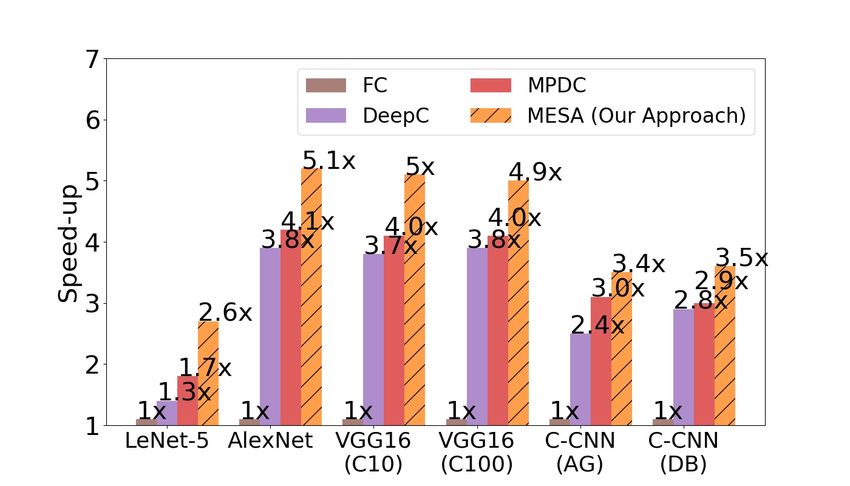
24th European Conference on Artificial Intelligence - ECAI 2020
                                                         Santiago de Compostela, Spain

also be well addressed to further compress the model. Consider a            works. Sec. 3 formulates the problem and discusses our observa-
given weight matrix that the weights are quantized to 3 bits, with          tions. Sec. 4 details the algorithm design, and Sec. 5 presents the
representing index in [0, 7], as shown in Fig. 1(c). Fig. 1(c) is well      experimental results. Finally, Sec. 6 concludes this paper.
arranged with correlated small entropy (the entropy value is 0) with
all the differences as 1 on all the 2 × 2 blocks, whereas the entropy       2      Related Works
value of Fig. 1(b) is 2.46 along the diagonal. By doing so, encod-          Compressing NN models has been actively studied in the past few
ing by the blocks’ pair-wise index differences in Fig. 1(c) leads to a      years. The main objective is to minimize the memory consumption
concentrated distribution as shown in Fig. 1(d). By applying lossless       in the inference phase with a very limited accuracy drop, where the
compression, such as Huffman coding, we only need 8 bits to encode          works can be basically categorized into quantization, pruning, and
the remaining matrix, while those in Figs. 1(a) and 1(b) require 82         low-rank approaches.
(with CSR and Huffman) and 30 bits, respectively.                              The quantization-based approaches, such as binarization quanti-
   With the observations above, in this paper, we aim to reduce the         zation [1], [23] and fixed-point quantization [16], [5], use fewer bits
model size by considering the block diagonal structure and the min-         to represent the original weights for reducing the memory consump-
imum data entropy of sequential block differences (minimum block-           tion. In addition, approaches that employ sharing index such as [21],
wise differences for short). Unlike most existing approaches, such as       [19] are also proposed to enable an efficient lookup mechanism for
pruning and quantization [1], [23], [16], [19], [6], [25], [24], that fo-   performance improvements.
cus only on removing redundant weights or reducing the allocated               For pruning-based approaches [6], [24], [25], [26], the less impor-
bits for weights, we make the first attempt to consider the structural      tant weights in the model are pruned to reduce the complexity. By
properties of the matrix to effectively reduce the memory consump-          putting pruning and quantization together, DeepCompression [21]
tion, which is particularly useful for embedded systems and mobile          proposed a three-stage pipeline with pruning, quantization, and Huff-
devices. To our best knowledge, this is the first work that considers       man coding for the quantized index. Further, MPDCompress [22]
the block diagonal structure with minimum block-wise differences            proposes to store the sparse weights as diagonal blocks to facilitate
to compress the model. It is worth noting that, although we present         parallel computation on GPU devices. However, since none of the
our results for fully-connected layers in this paper, our ideas can be      above works considers the structural factor to minimize the block-
easily extended to compress convolutional layers.                           wise differences in the weight matrix, our ideas and algorithms are
   Specifically, we formulate a new research problem, named                 complementary to these works for improving the compression rate.
COmpression with Difference-MInimized Block Diagonal Structure                 In addition, low-rank matrix factorization and tensor decomposi-
(COMIS) that takes as input an NN model and transforms it to a              tion are also employed for compression [15], [11]. Also, a recent line
memory-efficient representation (i.e., compressed model) with a lim-        of studies aims at reducing the vast convolutional layers by reformu-
ited accuracy drop. We design a new algorithm, named Memory-                lating its standard structure, such as SqueezeNet [9], MobileNet [7],
Efficient and Structure-Aware Compression (MESA), which employs             and EffNet [4].
the ideas of lottery ticket hypothesis and arbitrary pruning with a new        To summarize, although the above works achieve good perfor-
penalty function to minimize the block-wise differences in the block        mance, however, they do not consider the block diagonal structure
diagonal structure to significantly improve the compression rate. We        with the minimum block-wise differences, which are critical to fur-
conduct extensive experiments to validate our ideas and evaluate our        ther reduce the model size. In this paper, we make the first attempt to
algorithm. Our algorithm is able to achieve compression rates of            optimize the model compression by incorporating these ideas.
135× to 392× on various models, tripling the compression rates of
the state-of-the-art approaches [21], [22]. For the inference time, the     3      Problem Formulation and Analysis
models compressed by MESA achieve 2.6× to 5.1× speed-up com-
pared to the full precision model and up to 44% speed-up compared           Problem Formulation. The COMIS problem is formulated as fol-
to the state-of-the-art NN compression approaches [21], [22]. The           lows. We are given a neural network with n fully-connected layers4 ,
contributions of this paper are summarized below.                           a set of target pruning rates P = {p1 , · · · , pn } and a set of quantiza-
                                                                            tion bits Q = {q1 , · · · , qn } for each fully-connected layer, where pi
• We observe that the block diagonal structure with the minimized           of weights should be kept (i.e., (1 − pi ) of weights should be pruned)
  block differences is able to boost the compression rate and the           in each layer 1 ≤ i ≤ n, and all the weights in layer i are quantized
  inference speed for NN model compression, and we validate our             from 32-bit floating point numbers to qi bits of weight index5 . The
  observations with analysis on multiple models.                            goal of COMIS is to minimize the model size with a limited accuracy
• We propose a new research problem, named Compression with                 drop, such that the non-zero weights for each fully-connected layer
  Difference-Minimized Block Diagonal Structure (COMIS) prob-               are organized as non-overlapping blocks in the diagonal of the weight
  lem with a new algorithm, Memory-Efficient and Structure-Aware            matrix (diagonal requirement), and the block-wise differences of the
  Compression (MESA), to significantly improve the compression              adjacent blocks should be small (min-difference requirement).
  rate. This is the first work that compresses the NN model with a             Here, the parameters P = {p1 , · · · , pn } and Q = {q1 , · · · , qn }
  difference-minimized block diagonal structure, which is comple-           can be assigned to consider different scenarios. A smaller pi or qi
  mentary with most existing compression methods.                           may lead to a smaller model size. However, when pi or qi is set too
• Extensive experiments on multiple models are conducted. The re-           small, it becomes more difficult (or infeasible) to compress the model
  sults show that MESA achieves 135× to 392× compression rates,
                                                                            4   Even if the model contains both fully-connected and convolutional lay-
  tripling those of the state-of-the-art approaches. Additionally, the
                                                                                ers, the proposed COMIS problem and algorithm can still be applied to
  models compressed by MESA achieve 2.6× to 5.1× speed-up (in-
                                                                                compress the fully-connected layers. Moreover, our approach can be eas-
  ference time) compared to the full precision model, and up to 44%             ily extended to compress the convolutional layers by slightly changing the
  of speed-up compared to the state-of-the-art approaches.                      penalty function.
                                                                            5   P and Q can be set according to [21] and will be discussed in the experi-
  This paper is organized as follows. Sec. 2 discusses the relevant             ments section.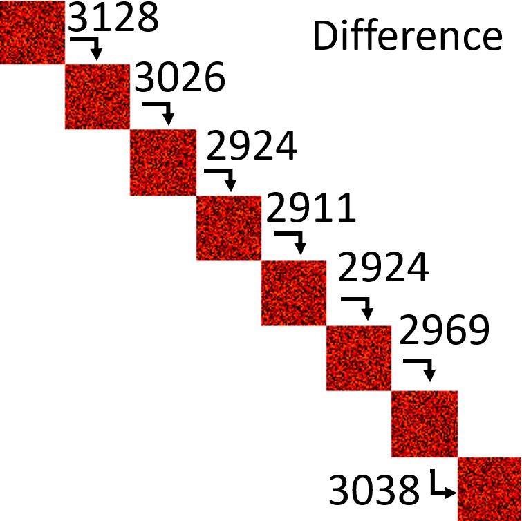
24th European Conference on Artificial Intelligence - ECAI 2020
                                                          Santiago de Compostela, Spain

with a limited accuracy drop. Since previous work has shown that the         DeepCompression for each individual layer (Arb). iii) Moreover, we
performance remains the same if the neural networks are compressed           prune the weights not residing in the blocks on the diagonal with the
with the same P and Q, the settings of P and Q are based on the              same pruning rate as in DeepCompression, which is a special case of
previous compression results by other approaches in practice, such           the arbitrary pruning strategy (referred to as Diag).
as DeepCompression [21], MPDCompress [22]. Please note that as                      Table 1.   Preliminary results for different pruning strategies
shown in the experimental results, our proposed approach signifi-                                     Pruning rates             DeepC    Arb      Diag
cantly outperforms DeepCompression and MPDCompress under the                     LeNet-5              10%, 20%                  99.35    99.03    99.11
same pi and qi settings.                                                         VGG16 CIFAR-10       12.5%, 12.5%, 10%         91.38    91.1     91.44
                                                                                 VGG16 CIFAR-100      12.5%, 12.5%, 10%         72.33    72.35    72.12
   In this paper, our proposed algorithm is able to prune the net-               AlexNet              10%, 10%, 25%             53.23    54.16    53.37
work more effectively to enhance the compression rate by satisfy-
ing the two requirements above, i.e., diagonal requirement and min-             The results are reported in Table 1, where the third, fourth, and
difference requirement, which are added to allow run-length coding           fifth columns in Table 1 respectively present the accuracy of the
to significantly reduce the model size, as illustrated in Fig. 1. These      model compressed by DeepC, Arb, and Diag, all with the same
requirements are designed to follow our observations below. Please           number of weights. Diag is very close to DeepC and Arb in all
note that, although our observations and ideas are presented with            models, which manifests that arbitrary pruning the same ratio of
fully-connected layers, the proposed ideas can be easily extended to         weights to generate block diagonal structure produces similar or bet-
compress the convolutional layers.                                           ter accuracy in these models. This observation validates the feasibil-
   Observations and Analysis. As mentioned earlier, arranging the            ity and effectiveness of transforming the weight matrix into a block
sparse matrix (representing the weights of a fully-connected layer)          diagonal structure for better model compression. Based on this im-
to a block diagonal structure is critical for effectively reducing           portant observation, we propose the algorithm for COMIS in the next
the model size. However, reducing the model size while satisfying            section.
the diagonal requirement is very challenging because conventional
pruning-based approaches, such as [25], [24], [26], usually fail to
                                                                             4    Algorithm Design
generate a pruned weight matrix where non-zero weights are grouped
into blocks on the diagonal. This is because they aim to prune out the       To solve the proposed COMIS problem, in this paper, we pro-
less important weights defined in their work, but such less important        pose algorithm Memory-Efficient and Structure-Aware Compression
weights often scatter irregularly in the weight matrix.                      (MESA), which includes four steps as detailed below.
   Recently, Frankle et al. and Liu et al. [17], [3] both point out             Step 1. Pruning with Block Diagonal Mask (PM). Given the
that given the assigned pruned model structure from the conven-              pruning rate pi of the i-th weight matrix, the conventional pruning
tional pruning-based approaches, the pruned network structure can            approaches [25], [24], [26], [6] identify the importance of the weights
be trained from scratch and provide a similar or even better model           and then prune the less important ones until the desired number of
accuracy. On top of that, Supic et al. [22] demonstrate the effective-       weights are pruned. Although these approaches may be able to re-
ness of arbitrary pruning strategy on fully-connected layers. In their       tain the accuracy eventually, there is no guaranteed structure for the
experiments, they show that given the percentage of weights to be            weight matrix after the pruning. Consider a running example in Fig.
pruned from each layer, one can arbitrarily prune off that number            2, given the weight matrix of size 4096 × 4096 and a pruning rate of
of weights (i.e., the arbitrary pruning strategy) and train the pruned       12.5%, a trivial pruning approach that keeps 12.5% of weights with-
network from scratch to provide a model accuracy comparable with             out considering the block diagonal structure may obtain the irregular
the original full-precision model. This observation motivates us to          sparse matrix as shown in Fig. 2(a). However, as mentioned earlier,
explore a new direction to effectively prune the weight matrix in or-        the block diagonal structure is critical to model efficiency. There-
der to extract the winning ticket subnetwork [3] (i.e., the subnetwork       fore, in the first step, after the pruning rate of each layer is identi-
that matches the test accuracy of the original network when trained          fied by the threshold pruning method (e.g., [6]), we directly train the
in isolation from scratch) from the original network while satisfying        block diagonal sparse matrix with a mask. In this way, the redun-
the diagonal requirement of the COMIS problem.                               dant weights can be structurally pruned and compressed. Compared
   To validate and gain more insights for the arbitrary pruning strat-       with unstructured pruning methods, block diagonal sparse matrix re-
egy, we conduct a preliminary experiment on 4 models, i.e., LeNet-5          quires no extra pointer to record the location of weights in the pruned
[14], VGG16 on CIFAR-10 [20], VGG16 on CIFAR-100 [20], and                   sparse matrix, which can further enhance the compression rate under
AlexNet [12]6 . For each model, we apply one of the state-of-the-            the same pruning rate of each layer. Furthermore, each block can be
art compression approaches, DeepCompression [21], and record its             independently computed to improve the parallelism of the model in-
pruning rate for each individual fully-connected layer without any           ference.
accuracy drop. The second column of Table 1 reports the pruning                 Specifically, for the i-th weight matrix Wi , we denote xi and yi the
rates of DeepCompression, which are then used as the hyperparame-            row and column sizes of Wi , respectively. Given pruning rate pi , we
ters for testing other approaches. For example, the pruning rates for        first generate a binary mask MiB that has the same size as Wi . The
LeNet-5 are 10% and 20%, indicating that DeepCompression keeps               mask MiB has b p1i c dense blocks assigned as 1 (binary True) along
10% and 20% of weights in the first and second fully-connected lay-          the diagonal. Each of the b p1i c dense blocks along the diagonal axis
ers, respectively. Moreover, in this pilot experiment, all the weights       in MiB has the size of (bxi · pi c) × (byi · pi c), and the remaining
for the compared approaches are quantized to 5 bits. For each model,         values outside the diagonal blocks are assigned as 0 (binary False).
we compare the performance of three approaches: i) DeepCompres-              Under the same pruning rate pi , each block is set to the same size
sion (DeepC) [21]; ii) The arbitrary pruning strategy to prune the           instead of using blocks with irregular sizes because of the following
fully-connected layers randomly with the same pruning rate as in             reasons: 1) When the blocks come with different sizes, extra infor-
6   We also present the experimental results on non-computer vision models   mation is required for recording the size of each block, while same-
    later in the experiments section.                                        sized blocks only need to record the size of the first block. 2) The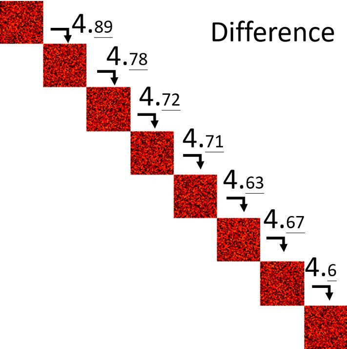
24th European Conference on Artificial Intelligence - ECAI 2020
                                                              Santiago de Compostela, Spain

   (a) Irregular sparse matrix (b) Diagonal blocks (step 1) (c) Minimized block-wise (d) Distribution of weight indices (e) Distribution of weight indices with
   (by trivial approach)                                  differences (step 2)          without delta-coding              delta-coding (step 3)

                       Figure 2. Running example on fc2 (second fully-connected layer) in VGG16 on CIFAR-10 (pruning rate: 12.5%)

memory needed for model inference is related to the largest dense                   aligning {B1i , B2i , · · · , Bbn
                                                                                                                   i
                                                                                                                      i
                                                                                                                        } sequentially along the diagonal axis.
block since the matrix multiplication can be processed by loading                                                i
                                                                                    Actually, since each Bj , ∀1 ≤ j ≤ bni , can be computed indepen-
the weights block-by-block. Therefore, the size of the blocks in each               dently, there is no need to reconstruct the original weight matrix. The
fully-connected layer is set to bxi · pi c × byi · pi c.                            pseudocode of our first step (PM) is presented in Algorithm 1.
   Next, we apply this mask and train the model from scratch. Each                     Step 2. Difference Minimization for Neighboring Blocks (DM).
mask MiB covers the weight matrix Wi , with an AND operation                        In step 1, for each WiM , ∀1 ≤ i ≤ n, only the blocks
masking out the weights not residing on the diagonal block structure.               {B1i , B2i , · · · , Bbn
                                                                                                          i
                                                                                                            i
                                                                                                              } are stored. Although this approach achieves
Let WiM be the weight matrix between layers i and i + 1 after the                   good compression rate, it still leaves a large room for further
mask is applied, WiM = Wi AND MiB . By applying the mask MiB ,                      improvement. After the weights in each Bji are quantized, we
we force the weights to propagate forward only if the corresponding                 can further minimize the block-wise differences between Bji and
position on the mask is assigned as 1 (binary True). This ensures that                i
                                                                                    Bj+1   , ∀j ∈ [1, bni − 1]. By doing so, we control the entropy of the
in the back-propagation stage, only the corresponding position with                 pair-wise distances between the blocks by concentrating the distance
binary True is updated, while other weights remain zero. The idea of                close to zero, and then in step 3, we can employ the delta-coding
applying this binary mask can be regarded as a special case of the                  techniques [8] to encode the differences to further reduce the model
arbitrary pruning strategy, which implements the operation similar to               size.
Diag in Table 1. Therefore, the model accuracy is not likely to incur
a sharp drop after applying this mask.                                              Example 2 Fig. 2(b) shows the masked weight matrix and the to-
                                                                                    tal difference of adjacent blocks without considering to minimize the
Example 1 Fig. 2 presents an example of pruning with the pro-
                                                                                    differences between adjacent blocks. In contrast, the same masked
posed block diagonal mask. After applying the generated mask on
                                                                                    weight matrix after minimizing the differences is shown in Fig. 2(c).
the weight matrix of size 4096 × 4096, the new matrix is shown in
                                                                                    The differences between adjacent blocks are reduced by approxi-
Fig. 2(b), which contains 8 non-overlapping blocks from top left to
                                                                                    mately 600 times in Fig. 2(c), as compared to Fig. 2(b). After quan-
bottom right. We also label the block-wise differences between adja-
                                                                                    tization, the minimized differences between the blocks shrink the en-
cent blocks in this figure.
                                                                                    tropy from 4.44 to 0.05.

Algorithm 1 Pruning with Block Diagonal Mask (PM)                                      Therefore, to minimize the block-wise differences between the ad-
Input: Fully-connected weight matrix: W with size (x × y), pruning rate p           jacent blocks, we propose a new penalty function, namely, Loss of
Output: Pruned fully-connected layer: W M                                           Distance Penalty LDP , as follows.
 1: Generate M B by the size of W , with b p1 c dense blocks assigned as
    binary True along the diagonal axis having the same size bx · pc × by · pc                                     n bni −1  i
                                                                                                                                − Bji ||2
                                                                                                                1 X X ||Bj+1
 2: W M ← W AND M B                                                                                     LDP =                             ,
 3: block-number: bn ← b p1 c                                                                                   n i=1 j=1   (bni − 1)
 4: return W M , bn
                                                                                    where n is the number of fully-connected layers, bni = b p1i c is the
   After training each weight matrix with the mask MiB , the original               number of diagonal blocks in the i-th masked weight matrix WiM
matrix is transformed into a new matrix such that only independent                  generated by step 1 (recall pi is the pruning rate of layer i), and Bji
blocks (with non-zero weights) exist on its diagonal. Given the prun-               is the j-th block in WiM . When the difference between Bji and Bj+1i
                                                                                          i
ing rate of the i-th weight matrix pi , let bni = b p1i c denote the block          or Bj−1    is large, the loss increases. Based on LDP , we design the
                                                                                    loss function Ltotal for training as follows.
number of the i-th weight matrix, and let {B1i , B2i , · · · , Bbni
                                                                    i
                                                                      } de-
note the blocks on the diagonal of the matrix in each fully-connected
layer i, where B1i is the top left block. Instead of storing the whole                                         Ltotal = Lacc + αLDP ,
weight matrix, considerable memory space can be saved by storing                    where Lacc is the accuracy loss7 , and α is a hyper-parameter de-
only the blocks {B1i , B2i , · · · , Bbn
                                      i
                                         i
                                           } of each masked weight ma-              signed to control the trade-off penalty between the compression rate
        M
trix Wi . This is because the locations of the non-zero weights are                 and the model accuracy. A larger α value allows the normalization
pre-defined, i.e., they are arranged into same-sized blocks on the di-
                                                                                    7
agonal, and thus we can easily reconstruct the original weights by                      Loss can be cross-entropy or MSE according to the learning task.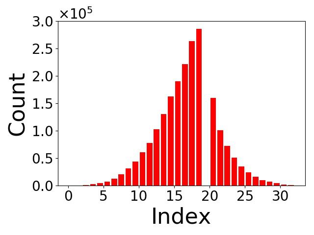
24th European Conference on Artificial Intelligence - ECAI 2020
                                                           Santiago de Compostela, Spain

factor to become more dominant which makes the blocks more sim-                number of blocks in WiB . Our algorithm then outputs the encoded
ilar and more likely to be quantized with the same code. Thus, the             B1i block along with the (bni − 1) delta-coded sequence for each
compression rate becomes higher with delta-coding since the en-                fully-connected layer i as the final compressed model.
tropy of the delta weight distribution is smaller, enabling Huffman
coding to be more memory-efficient. In contrast, a smaller α allows            Example 4 For VGG16 on CIFAR-10 in Fig. 2, if each weight is
the weights to be more likely to fit the original error loss and thus          quantized to 5 bits, the weights of the fully-connected layers consume
the model accuracy can be higher, since minimizing the error loss              10 MB of memory. After steps 1-3, the model is compressed to 1.25
becomes a more important factor in the loss function.                          MB. If encoded with cyclic-distance in step 3, the compressed model
   In practice, when the goal is to achieve the best compression rate          (after Huffman coding) takes 394 KB, while the model size (after
without accuracy loss, α is set as large as possible until the accuracy        Huffman coding) is 901 KB without cyclic-distance delta-coding.
drops. On the other hand, in the case that the memory or bandwidth                In our experiments, by employing Huffman coding on the cyclic-
is extremely limited and slight accuracy loss can be tolerated, α can          distance delta-coding, our approach outperforms the direct encoding
be set as a large value to strike a good balance between the accu-             with quantized indices by reducing up to 60% of the model size.
racy requirement and the size of the model. As Ltotal considers the            The pseudocode of step 3 is presented in Algorithm 3. Finally, com-
similarity between blocks as a chain and therefore after the model             bining the 4 steps altogether, the pseudocode of algorithm MESA is
converges, reorganizing the sequence of delta-coded blocks is not              presented in Algorithm 4.
necessary for the subsequent steps. The pseudocode of our second
step (DM) is listed in Algorithm 2.                                            Algorithm 3 Post-Quantization Cyclic-distance Assignment (PQA)
                                                                               Input: Quantized diagonal blocks: B ∗ , B , maximum weight index range: r
Algorithm 2 Difference Minimization for Neighboring Blocks (DM)                Output: Delta-encoded form of B ∗ : B R
Input: Masked weights for each layer: W = {W1M , · · · , WnM }, block           1: B R = size(B ∗ )
    number for each layer: BN = {bn1 , · · · , bnn }                            2: for i, j in size of B ∗ do
                                                                                          R                ∗                  ∗
Output: Loss of Distance Penalty: (LDP )                                        3:     Bi,j   ← min{|Bi,j     − Bi,j |, r − |Bi,j − Bi,j |}
 1: i ← 1, j ← 1, LDP ← 0                                                       4: return B R
 2: for i ≤ n do
 3:     for j < bni do
                                 i
                              ||Bj+1 −Bji ||2
 4:         LDP ← LDP +           bni −1                                       Algorithm 4 Memory-Efficient and Structure-Aware Compression
 5:        j ←j+1                                                              (MESA)
 6: return LDP                                                                 Input: n, W = {W1 , · · · , Wn }, P = {p1 , · · · , pn }, Q = {q1 , · · · , qn }
                                                                               Output: Compressed NN weights after MESA is applied: W C
                                                                                1: for each NN layer Wi do
   Steps 3 and 4. Post-Quantization Cyclic-distance Assignment                  2:     WiM , bni ← PM(Wi , pi ), initialize pruned weights WiM
(PQA) and Huffman Encoding with Organized Distribution                          3: For each layer, BN ← all bni ; W M ← all WiM
(HE). At step 3, after the model converges, we quantize the weight              4: for each training epoch do
                                                                                5:     Input batch data and calculate the M SE
matrix of each fully-connected layer i according to the given param-            6:     Loss ← M SE ; Loss ← Loss + DM(W M ,BN )
eter qi with the k-means clustering algorithm and train the model               7:     Compute gradient, back propagation
until it recovers the accuracy. Next, for the bni sequence of blocks            8: for each Converged weight: WiM do
                                                                                9:     WiM ← Quantized WiM from 32 bits to qi bits
Bji in the i-th fully-connected layer, we delta-code B2i to Bbni
                                                                 i
                                                                   by          10: for each Quantized weight matrix: WiM do
the cyclic-distance of the quantized index from its previous block on          11:     range ← 2qi
the diagonal. For example, given two (1 × 2) 3-bit quantized blocks,           12:     for j from 1 to (bni − 1) do
                                                                                              i              i
µ1 and µ2 , where µ1 = [0, 1] and µ2 = [7, 1]. µ2 in this case is              13:         Bj+1   ← PQA(Bj+1      , Bji , range)
                                                                               14:     Compressed weight WiC ← Huffman code B1i and {B1i , · · · , Bm       i
                                                                                                                                                               } re-
delta-coded as [−1, 0] to ensure that the bit range remains the same
                                                                                   spectively from WiM
as encoded by the original quantized bits.                                     15: return Compressed NN weights W C
   Putting penalty, quantization, and cyclic-distance delta-coding to-
gether, we can adjust carefully the differences between adjacent
blocks to make each block more similar to its nearby blocks and
can also encode cyclic-distance between blocks after quantization,             5    Experimental Results
where cyclic-distance is concentrated in a small range as shown in             Models and Datasets. We compare our algorithm with other base-
Fig. 2(e). The concentrated distribution can be further compressed             lines on multiple NN models. Similar to most model compression
by run-length coding, e.g., Huffman coding in the next step.                   works, well-known computer vision models and datasets are used,
                                                                               including LeNet-5 on MNIST (LeNet-5 for short) [14], VGG16 on
Example 3 Continue our running example in Fig. 2, where Fig. 2(c)
                                                                               CIFAR-10 and CIFAR-100 (VGG16 (C10) and VGG16 (C100) for
shows the blocks (and the total of their difference values) after step
                                                                               short, respectively) [20], AlexNet on CIFAR-100 (AlexNet for short)
2. After the quantization mentioned above, the distributions of the
                                                                               [12], and AlexNet on ImageNet (AlexNet (ImageNet) for short) [10].
weight indices and the cyclic-distance weights indices are shown in
                                                                                  In addition, to demonstrate that the proposed approach can be ap-
Figs. 2(d) and 2(e), respectively.
                                                                               plied to the NN models for other tasks, we conduct experiments on
   At step 4, the last step, we generate two codebooks using Huff-             predicting the category of the input text content with Char-ConvNet
man coding for each fully-connected layer. The first codebook en-              [28] on AG’s News and DBPedia, abbreviated as C-CNN (AG) and
codes the absolute indices of the first block in each masked fully-            C-CNN (DB), respectively. Char-ConvNet comprises 6 convolutional
connected layer, i.e., B1i in WiB , and the second codebook encodes            layers and 3 FC layers. AG’s News dataset from web8 contains news
the differences of block-wise indices along the diagonal block se-             8     http://www.di.unipi.it/˜gulli/AG_corpus_of_news_
quence, i.e., ||B2i − B1i ||, · · · , ||Bbn
                                         i
                                           i
                                                i
                                             − Bbn i −1
                                                        ||, where bni is the       articles.html.
24th European Conference on Artificial Intelligence - ECAI 2020
Santiago de Compostela, Spain
articles in 4 categories, where each category contains 30000 training
samples and 1900 testing samples. Moreover, DBPedia dataset con-
tains 14 non-overlapping ontology classes from DBPedia 2014 with
each class having 40000 random training samples and 5000 testing
samples.
Baselines. We compare the proposed MESA with five other baselines:
i) DeepCompression (DeepC) [21], one of the state-of-the-art al-
gorithms that effectively compresses the deep neural networks; ii)
MPDCompress (MPDC) [22], which is able to achieve high compres-
sion rates by considering the block diagonal structure of the weights,
but does not consider to minimize the block-wise differences be-
tween adjacent blocks; iii) MPDCompress with quantization and
Huffman coding (M+Q+H), which quantizes the weight matrix com-
pressed by MPDC to 5 bits, then encodes the quantized weights with
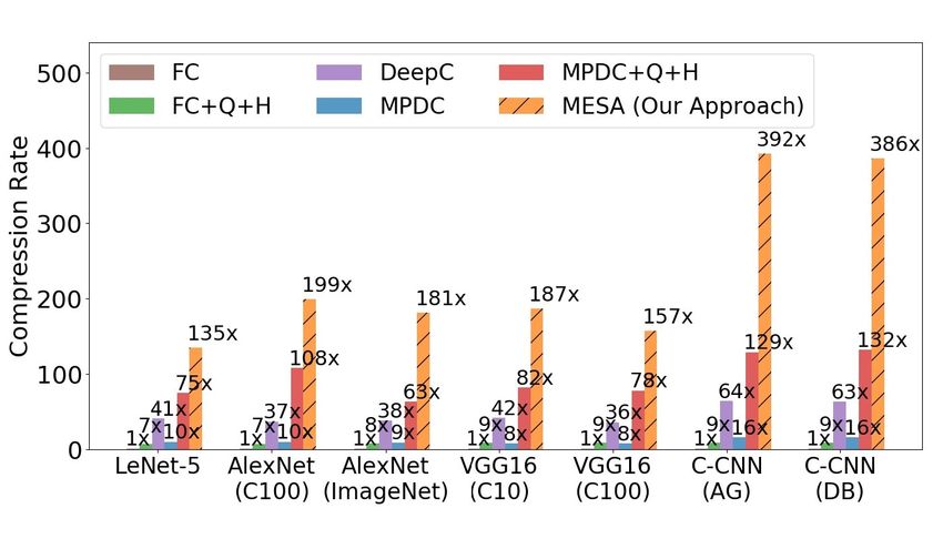
the absolute quantization indices, and applies Huffman coding on the Figure 3. Compression rates of different approaches
quantized indices; iv) Original fully-connected layer (FC), which is
the comparison basis with no operation performed on the weights; v) is listed in Table 2. The compression rates are calculated based on the
Original fully-connected layer with quantization and Huffman cod- weights of the original fully-connected layer (FC) without any com-
ing (FC+Q+H), which quantizes the original weights to 5 bits and pression. MESA significantly outperforms the other baselines on all
then applies Huffman coding on them without pruning any weights. the models. Its compression rates range from 135× to 392× due to
For fair comparisons, we set all quantization bits qi of MESA to 5 the different pruning rates of the models, which vary significantly ac-
bits according to the suggestions from DeepCompression [21], which cording to the redundancy of each model. For example, VGG16 and
strikes a good balance between the compression rate and accuracy9 . AlexNet do not have any accuracy drop when keeping only 12.5%
Moreover, MESA and all the baseline approaches are trained to allow (8× compression) and 10% (10× compression) of weights, respec-
only a tiny accuracy drop as compared to FC, i.e., within 1%, in the tively. For C-CNN on both datasets, the fully-connected layers can
experiments. be pruned to keep only 6.5% (16× compression) of weights while
Measures. For fair comparisons, the pruning rates (p) for each retaining the same accuracy.
model, i.e., the ratio of the number of the remaining weights to that of We further analyze the compression rates of MESA contributed
the original weights, are set the same as those for threshold pruning by different steps. First, after performing steps 2-4 of MESA, the
methods. More specifically, For LeNet-5 and AlexNet (ImageNet), delta-coding on the difference-minimized blocks along with the sub-
we set the pruning rates according to those reported in DeepCom- sequent Huffman coding introduces the extra 2.1×, 2.3×, 3.1×,
pression [21]. For VGG16 (C10), VGG16 (C100), C-CNN (AG), C- 3.65×, 3.06×, 3.8×, and 3.7× compression rates on AlexNet,
CNN(DB), and AlexNet, we set the pruning rates such that Deep- AlexNet (ImageNet), LeNet-5, VGG16 (C10), VGG16 (C100), C-
Compression [21] has its accuracy loss within 1% compared to the CNN (AG), and C-CNN (DB), respectively. Please note that Huff-
original uncompressed models (our proposed approach also has ac- man coding achieves only about 1.5× compression rate in other
curacy loss within 1%). Moreover, Average bits (avg. bits) denotes baselines, which indicates that our idea of delta-coding on the blocks
the model size (in bits) divided by the total number of unpruned with minimized block-wise differences indeed facilitates the perfor-
weights, which shows how many bits are needed for the informa- mance of Huffman coding.
tion of each unpruned weight (including the pointers to locate the On the other hand, MPDC, which constructs block diagonal struc-
weights if any). Compression Rate (CP Rate) measures the overall ture by permutation, shows low (8× to 16×) compression rates be-
performance of the compression algorithms. Similar to most works cause the block diagonal structure of MPDC is mainly used to improve
in neural network compression [27, 2], our algorithm and the com- the efficiency of matrix multiplication instead of generating blocks
pared baselines only compress the weights in the fully-connected lay- with minimized block-wise differences. To understand how quanti-
ers. Therefore, the compression rate is calculated as the memory size zation and Huffman coding can enhance MPDC, we also present the
of the original weights in the fully-connected layers, divided by the results of M+Q+H, which show a significant improvement on the com-
memory size of the compressed fully-connected layers generated by pression rates (75× to 132×) compared to MPDC. However, without
the compression algorithm (including the codebook size if any). A minimizing block-wise differences on the block diagonal structure,
larger compression rate indicates a better performance for the algo- the compression rates are still much inferior to those of MESA.
rithm. FC+Q+H is compared to show the performance of quantization
The experiments are conducted with Pytorch 0.4.1 framework. and Huffman coding, which has only 7× to 9× compression rates,
The models are trained on a server equipped with a 3.60 GHz In- where 6.4× of compression rate is contributed by quantization. Since
tel Core i7-7700 CPU, a GeForce RTX 2080Ti, and 64 GB RAM. the weight matrices are neither pruned nor rearranged to optimize the
The default α (hyper-parameter for penalty) is 0.1. performance of Huffman coding, Huffman coding contributes a very
limited compression rate, from 1.09× to 1.4×. Finally, DeepC, one
5.1 Compression Rates of the state-of-the-art compression algorithm, achieves 36× to 64×
compression rates. The pruning and its CSR (or CSC) format effec-
Fig. 3 compares the compression rates of the proposed MESA with tively reduce the model sizes. However, since i) CSR (or CSC) for-
other baselines, while the corresponding accuracy of each approach mats require additional information to locate the non-zero weights,
9 It is possible to set different quantization bits for different fully-connected
and ii) DeepC does not jointly consider the pruning and quantiza-
layers, which can be viewed as a hyper-parameter optimization problem. tion for optimizing the compression rate of Huffman coding, there is
We leave the discussion of this topic in the future work. a large gap between DeepC and MESA on the compression rates.24th European Conference on Artificial Intelligence - ECAI 2020
Santiago de Compostela, Spain
Table 2. Accuracy of different approaches
FC FC+Q+H DeepC MPDC M+Q+H MESA
LeNet-5 99.34 99.28 99.29 99.08 99.03 99.04
VGG16 (C10) 91.32 91.40 91.44 91.14 90.53 91.14
VGG16 (C100) 71.40 72.33 72.57 71.84 71.91 71.46
AlexNet 52.68 52.77 54.04 53.69 53.83 53.47
AlexNet (ImageNet) 77.12 76.51 77.58 76.38 76.27 76.55
C-CNN (AG) 86.61 86.68 86.76 86.51 87.22 87.21
C-CNN (DB) 97.84 97.90 97.94 97.92 98.05 97.92
5.2 Layer-wise Statistics of Different Models
Table 3. Layer-wise average bits in LeNet-5
DeepC M+Q+H MESA MESA Figure 4. Inference speed-up of different approaches
Size p
Avg. Avg. bits Avg. CP
bits bits Rate
fc1 1.52MB 10% 7.6 4.2 2.3 138×
fc2 19.53KB 10% 14.2 6 6.7 47× reach their pruning and quantization limits, weight distribution ad-
total 1.54MB 10% 7.7 3.1 2.3 135× justment (in step 2 of the algorithm) by MESA still provides extra
compression. The block-wise delta coding between adjacent blocks
provides over 3× memory size reduction compared to M+Q+H. All
LeNet-5 on MNIST. In the following, Size represents the orig- together, C-CNN compressed by MESA requires only around 1.3 bits
inal size of the 32-bit float representation of the weights in fully- for each non-zero weight, and the compression rate can be as high as
connected layers. For LeNet-5, as shown in Table 2, MESA achieves 392× for AG’s news.
the accuracy of 99.04% with a slight accuracy drop compared to the
original FC with 99.34% accuracy. Table 3 presents the average bits Table 5. Layer-wise average bits in C-CNN (DB)
for each approach. MESA outperforms the other baselines in average
bits. In fc1 (the first fully-connected layer), DeepC requires 7.6 av-
erage bits because additional bits are required to locate the non-zero
weights in the sparse matrix. While M+Q+H lowers the average bits DeepC M+Q+H MESA MESA
Size p
Avg. Avg. bits Avg. CP
to 4.2 bits, it still consumes nearly twice memory compared to MESA bits bits Rate
(2.3 bits). fc1 34MB 6.25% 8.0 3.9 1.3 396×
One may observe that the average bits for fc2 (the second fully- fc2 4MB 6.25% 9.2 4.0 1.4 361×
connected layer) are high for all the algorithms. This is a special case fc3 56KB 50% 4.7 1.8 2.3 28×
total 38.05MB 6.38% 8.1 3.8 1.3 386×
where the fully-connected layer after pruning becomes too small, and
the codebook overhead dominates the representation. For example, in
fc2, the codebook consumes 103 Bytes, but only 29 Bytes are needed
C-CNN on DBPedia. For C-CNN on DBPedia, the average bits
to represent the weights by MESA. Even so, MESA still achieves a
for non-zero weights in fc3 of MESA is slightly larger than M+Q+H.
47× compression rate in fc2.
This is because when our Loss of Distance Penalty (LDP ) minimizes
the distances, it may sometimes sacrifice the compression rate of the
Table 4. Layer-wise average bits in C-CNN (AG) much-smaller fully-connected layers in order to reduce the accuracy
loss. However, this does not affect the performance of the overall
compression rate for MESA. The overall average bits for model com-
DeepC M+Q+H MESA MESA pressed by MESA is still around 3× smaller than M+Q+H and 6.2×
Size p
Avg. Avg. bits Avg. CP smaller than DeepC. For the layer-wise average bits of VGG16 and
bits bits Rate AlexNet, they show similar trends to the models described above
fc1 34MB 6.25% 7.9 3.9 1.3 401×
fc2 4MB 6.25% 8.9 4.1 1.5 341× where MESA outperforms all other baselines significantly. We omit
fc3 16KB 25% 9.8 5.3 4.2 31× the results due to their similarity trends.
total 38.01MB 6.28% 8 3.95 1.3 392× In summary, the results on NLP datasets (C-CNN on AG’s News
and DBPedia) are better than those on image datasets (CIFAR-10 and
CIFAR-100) since visual features are more complicated than sen-
C-CNN on AG’s news. Table 4 compares the results of MESA and tence embeddings, and it is thus more effective to diagonalize the
other baselines for text classification tasks. We observe that the layer- weight matrix of the NN for extracting features from NLP datasets.
wise pruning rates for the first two fully-connected layers, i.e., p1 , p2 ,
for C-CNN can be set to 6.25% without an accuracy drop. This indi-
5.3 Inference Speed-up on GPU
cates that the weights for fc1 and fc2 in C-CNN have a much higher
redundancy on AG’s News compared to other models. One major As mentioned earlier, the block diagonal structure can also improve
advantage of MESA is that even the baseline compression methods the efficiency of model inference. To validate this claim, we present24th European Conference on Artificial Intelligence - ECAI 2020
Santiago de Compostela, Spain
indices are 0 when α = 0.001, resulting in a very low entropy value
for its distribution, as shown in Table 6. Therefore, a larger α value
does not significantly improve the compression rate.
Table 6. Layer-wise data entropy on LeNet-5 and VGG16
LeNete-5 VGG16 (C10)
(a) LeNet-5 (b) VGG16 (C10) Orig. Delta-coded index Orig. Delta-coded index
index α=0.01 α=0.1 α=1.0 index α=0.001 α=0.01 α=1.0
fc1 4.86 4.58 3.39 2.00 2.94 0.2 0.07 0.1
fc2 4.97 4.91 4.85 3.42 2.81 0.08 0.03 0.08
fc3 N/A N/A N/A N/A 3.35 2.22 0.95 0.21
Figure 5. Penalty evaluation
6 Conclusion and Future Work
the inference time of the models compressed by MESA and other
baseline approaches. Here, speed-up represents the ratio of the in- In this paper, we propose the COMIS problem to consider the block-
ference time of the original uncompressed model (FC) to the infer- wise differences in block diagonal structure for NN model com-
ence time of the model compressed by a certain approach. A larger pression. We devise algorithm MESA, which effectively prunes the
speed-up value indicates a smaller inference time compared to the weights into a block diagonal structure and minimizes the block-
uncompressed model, i.e., FC. The inference time of each model is wise differences to boost the compression rate. Experiments show
calculated on a single GeForce RTX 2080Ti with CUDA 10.0. We that MESA achieves up to 392× compression rates, tripling those
employ cuBLAS GEMV kernel on the dense layers in FC and each of the state-of-the-art approaches, while significantly improving the
dense blocks in MPDC and MESA. For DeepC, each sparse layer is inference efficiency. In the future, we plan to explore the ideas of
stored in CSR format and cuSPARSE CSRMV kernel is used for i) fully leveraging the block-diagonal structure to reduce the mem-
general unstructured matrix operations in CSR format10 . ory access on ASIC, ii) learning to adaptively adjust the prun-
Fig. 4 shows that the speed-up of MESA outperforms the other ing rates/quantization bits for each layer of different models, and
baselines, i.e., the average speed-up of MESA, DeepC, and MPDC iii) proposing/experimenting different penalty functions for different
are 4.08×, 2.97×, and 3.28×, respectively. The speed-up of MESA models/datasets.
is around 26% higher than MPDC because the pruned fully-connected
layers of MESA are originally trained with block diagonal structure ACKNOWLEDGEMENTS
and do not require inverse matrix permutations to reconstruct the out-
put, which allows a better scheduling and memory organization. Yet, This work was supported in part by Ministry of Science and Technol-
MPDC still shows 10% better speed-up results compared to DeepC ogy (MOST), Taiwan, under MOST 109-2636-E-007-019-, MOST
because the latency of inverse permutations is minor compared to the 108-2636-E-007-009-, MOST 108-2218-E-468-002-, MOST 107-
reduced time of model inference with block diagonal structure. 2218-E-002-010-, MOST 108-2218-E-009-050-, and MOST 108-
2218-E-009-056-.
5.4 Penalty Evaluation
REFERENCES
To understand the impact of α, i.e., the hyper-parameter controlling [1] Yash Akhauri, ‘Hadanets: Flexible quantization strategies for neural
the trade-off between the accuracy and compression rate, we present networks’, arXiv preprint arXiv:1905.10759, (2019).
the compression rates of MESA with different α values on LeNet-5 [2] Yoojin Choi, Mostafa El-Khamy, and Jungwon Lee, ‘Universal deep
and VGG16 (C10). Fig. 5 shows that the compression rates increase neural network compression’, in arXiv preprint arXiv:1802.02271,
(2018).
significantly without obvious accuracy drops as α increases. With a [3] Jonathan Frankle and Michael Carbin, ‘The lottery ticket hypothesis:
larger α, the weights in adjacent blocks are easily to be quantized Finding sparse, trainable neural networks’, in International Conference
into the same index, and the weight distribution after delta-coding on Machine Learning, (2019).
can thus become more skew with a lower entropy. Table 6 shows [4] Ido Freeman, Lutz Roese-Koerner, and Anton Kummert, ‘Effnet: An
the entropy of the delta-coded weight distribution for LeNet-5 and efficient structure for convolutional neural networks’, in IEEE Interna-
tional Conference on Image Processing, (2018).
VGG16 (C10). For LeNet-5, when α equals to 1, the entropy values [5] Suyog Gupta, Ankur Agrawal, Kailash Gopalakrishnan, and Pritish
of fc1 and fc2 decrease from 4.86 and 4.97 to 2 and 3.42, respec- Narayanan, ‘Deep learning with limited numerical precision’, in Inter-
tively (LeNet-5 has only two fc layers). Please note that α controls national Conference on Machine Learning, (2015).
the trade-off and cannot be set too large. For example, setting α = 10 [6] Song Han, Jeff Pool, John Tran, and William Dally, ‘Learning both
weights and connections for efficient neural network’, in Advances in
for LeNet-5 and VGG16 (C10) results in an accuracy drop of more Neural Information Processing Systems, (2015).
than 1%. Fig. 5(b) shows that in VGG16 on CIFAR-10, MESA works [7] Andrew G Howard, Menglong Zhu, Bo Chen, Dmitry Kalenichenko,
well with a small penalty, i.e., α = 0.001, while the model accu- Weijun Wang, Tobias Weyand, Marco Andreetto, and Hartwig Adam,
racy retains (original model accuracy: 91.32%). When α becomes ‘Mobilenets: Efficient convolutional neural networks for mobile vision
larger, the compression rate of MESA, although outperforming other applications’, arXiv preprint arXiv:1704.04861, (2017).
[8] James J Hunt, Kiem-Phong Vo, and Walter F Tichy, ‘Delta algorithms:
baselines as shown in Fig. 3, does not improve significantly. After An empirical analysis’, ACM Transactions on Software Engineering
a careful examination, we find that 98% of the delta-coded weight and Methodology, (1998).
[9] Forrest N Iandola, Song Han, Matthew W Moskewicz, Khalid Ashraf,
10 Please note that CUDA libraries do not support the indirect lookup for William J Dally, and Kurt Keutzer, ‘Squeezenet: Alexnet-level accuracy
the quantized models. Therefore, we present the comparison results on the with 50x fewer parameters and < 0.5 mb model size’, in arXiv preprint
compressed model without quantization. arXiv:1602.07360, (2016).24th European Conference on Artificial Intelligence - ECAI 2020
Santiago de Compostela, Spain
[10] S. Satheesh H. Su A. Khosla J. Deng, A. Berg and L. Fei-Fei, ‘Ilsvrc- tations, (2019).
2012’, in http://www.image-net.org/challenges/ [20] Karen Simonyan and Andrew Zisserman, ‘Very deep convolutional net-
LSVRC/2012/, (2019). works for large-scale image recognition’, in International Conference
[11] Yong-Deok Kim, Eunhyeok Park, Sungjoo Yoo, Taelim Choi, Lu Yang, on Learning Representations, (2015).
and Dongjun Shin, ‘Compression of deep convolutional neural net- [21] Han Song, Huizi Mao, and William J Dally, ‘Deep compression: Com-
works for fast and low power mobile applications’, in International pressing deep neural networks with pruning, trained quantization and
Conference on Learning Representations, (2016). huffman coding’, in International Conference on Learning Representa-
[12] Alex Krizhevsky, Ilya Sutskever, and Geoffrey E Hinton, ‘Imagenet tions, (2016).
classification with deep convolutional neural networks’, in Advances [22] Lazar Supic, Rawan Naous, Ranko Sredojevic, Aleksandra Faust, and
in Neural Information Processing Systems, (2012). Vladimir Stojanovic, ‘Mpdcompress-matrix permutation decomposi-
[13] Nicholas D Lane, Sourav Bhattacharya, Akhil Mathur, Petko Georgiev, tion algorithm for deep neural network compression’, in arXiv preprint
Claudio Forlivesi, and Fahim Kawsar, ‘Squeezing deep learning into arXiv:1805.12085, (2018).
mobile and embedded devices’, IEEE Pervasive Computing, (2017). [23] Yaman Umuroglu, Nicholas J Fraser, Giulio Gambardella, Michaela
[14] Yann LeCun, LD Jackel, Leon Bottou, A Brunot, Corinna Cortes, Blott, Philip Leong, Magnus Jahre, and Kees Vissers, ‘Finn: A
JS Denker, Harris Drucker, I Guyon, UA Muller, Eduard Sackinger, framework for fast, scalable binarized neural network inference’, in
et al., ‘Comparison of learning algorithms for handwritten digit recog- Proceedings of the ACM/SIGDA International Symposium on Field-
nition’, in International Conference on Artificial Neural Networks, Programmable Gate Arrays, (2017).
(1995). [24] Qing Yang, Wei Wen, Zuoguan Wang, Yiran Chen, and Hai Li, ‘Integral
[15] Dongsoo Lee, Se Jung Kwon, Byeongwook Kim, and Gu-Yeon pruning on activations and weights for efficient neural networks’, in
Wei, ‘Learning low-rank approximation for cnns’, arXiv preprint International Conference on Learning Representations, (2019).
arXiv:1905.10145, (2019). [25] Shaokai Ye, Tianyun Zhang, Kaiqi Zhang, Jiayu Li, Kaidi Xu, Yunfei
[16] Zhisheng Li, Lei Wang, Shasha Guo, Yu Deng, Qiang Dou, Haifang Yang, Fuxun Yu, Jian Tang, Makan Fardad, Sijia Liu, et al., ‘Progressive
Zhou, and Wenyuan Lu, ‘Laius: An 8-bit fixed-point cnn hardware in- weight pruning of deep neural networks using admm’, in International
ference engine’, in IEEE International Symposium on Parallel and Dis- Conference on Learning Representations, (2019).
tributed Processing with Applications and IEEE International Confer- [26] Ruichi Yu, Ang Li, Chun-Fu Chen, Jui-Hsin Lai, Vlad I Morariu, Xin-
ence on Ubiquitous Computing and Communications, (2017). tong Han, Mingfei Gao, Ching-Yung Lin, and Larry S Davis, ‘Nisp:
[17] Zhuang Liu, Mingjie Sun, Tinghui Zhou, Gao Huang, and Trevor Dar- Pruning networks using neuron importance score propagation’, in IEEE
rell, ‘Rethinking the value of network pruning’, in International Con- Conference on Computer Vision and Pattern Recognition, (2018).
ference on Learning Representations, (2019). [27] Xiyu Yu, Tongliang Liu, Xinchao Wang, and Dacheng Tao, ‘On com-
[18] Antonio Polino, Razvan Pascanu, and Dan Alistarh, ‘Model compres- pressing deep models by low rank and sparse decomposition’, in IEEE
sion via distillation and quantization’, in International Conference on Conference on Computer Vision and Pattern Recognition, (2017).
Learning Representations, (2018). [28] Xiang Zhang, Junbo Zhao, and Yann LeCun, ‘Character-level convolu-
[19] Günther Schindler, Wolfgang Roth, Franz Pernkopf, and Holger tional networks for text classification’, in Advances in neural informa-
Fröning, ‘N-ary quantization for cnn model compression and infer- tion processing systems, pp. 649–657, (2015).
ence acceleration’, in International Conference on Learning Represen-You can also read