3D Human Pose Estimation Based on a Fully Connected Neural Network With Adversarial Learning Prior Knowledge - Frontiers
←
→
Page content transcription
If your browser does not render page correctly, please read the page content below
ORIGINAL RESEARCH
                                                                                                                                           published: 24 February 2021
                                                                                                                                        doi: 10.3389/fphy.2021.629288

                                             3D Human Pose Estimation Based on a
                                             Fully Connected Neural Network With
                                             Adversarial Learning Prior Knowledge
                                             Lu Meng * and Hengshang Gao
                                             College of Information Science and Engineering, Northeastern University, Shenyang, China

                                             3D human pose estimation is more and more widely used in the real world, such as sports
                                             guidance, limb rehabilitation training, augmented reality, and intelligent security. Most
                                             existing human pose estimation methods are designed based on an RGB image obtained
                                             by one optical sensor, such as a digital camera. There is some prior knowledge, such as
                                             bone proportion and angle limitation of joint hinge motion. However, the existing methods
                                             do not consider the correlation between different joints from multi-view images, and most
                                             of them adopt fixed spatial prior constraints, resulting in poor generalizations. Therefore, it
                                             is essential to build a multi-view image acquisition system using optical sensors and
                                             customized algorithms for a 3D reconstruction of the human pose in the image. Inspired by
                                             generative adversarial networks (GAN), we used a data-driven method to learn the implicit
                                             spatial prior information and classified joints according to the natural connection
                         Edited by:
                        Lijun Huang,
                                             characteristics. To accelerate the proposed method, we proposed a fully connected
            Huaihua University, China        network with skip connections and used the SMPL model to make the 3D human body
                        Reviewed by:         reconstruction. Experimental results showed that compared with other state-of-the-art
                           Haifeng Hu,
                                             methods, the joints’ average error of the proposed method was the smallest, which
University of Shanghai for Science and
                   Technology, China         indicated the best performance. Moreover, the running time of the proposed method was
                        Jianming Wen,        1.3 seconds per frame, which may not meet real-time requirements, but is still much faster
           Kennesaw State University,
                         United States
                                             than most existing methods.
                *Correspondence:             Keywords: 3D human pose estimation, fully connected neural network, hourglass network, SMPL model, generative
                         Lu Meng             adversarial networks
             menglu1982@gmail.com

                    Specialty section:       INTRODUCTION
         This article was submitted to
                Optics and Photonics,        Human pose estimation (HPE) refers to the detection and positioning of the joint points of the
               a section of the journal      people from the given optical sensor (cameras) input via algorithms. Estimating human pose is the
                   Frontiers in Physics.
                                             key to analyzing human behavior. HPE is the basic research in computer vision, which can be applied
      Received: 14 November 2020             to many applications, such as Human-computer interaction, human action recognition [1–4],
        Accepted: 04 January 2021
                                             intelligent security, motion capture, and action detection [5].
       Published: 24 February 2021
                                                3D human pose estimation methods were roughly categorized into two types: 1) predicting the 3D
                             Citation:       human pose from the RGB image in an end-to-end manner; 2) two-stage methods, in which the 2D
Meng L and Gao H (2021) 3D Human
                                             human pose was estimated from the RGB image firstly, and then the 3D human pose was predicted
   Pose Estimation Based on a Fully
     Connected Neural Network With
                                             based on the results of the 2D human pose.
Adversarial Learning Prior Knowledge.           Rogez et al. [6] presented an end-to-end architecture, named LCR-Net. The network included
               Front. Phys. 9:629288.        positioning, classification, and regression. First, the candidate human body regions were obtained by
     doi: 10.3389/fphy.2021.629288           the candidate pose region generator, and the potential poses were located in the candidate regions.

Frontiers in Physics | www.frontiersin.org                                         1                                        February 2021 | Volume 9 | Article 629288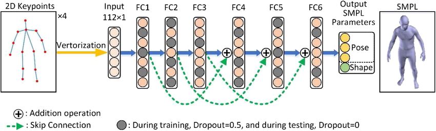
Meng and Gao                                                                                                             Human Pose Estimation

Scores of pose proposals were counted by the classifier. Finally,
the 3D human poses were obtained by regression. Pavlakos et al.
[7] directly regressed the 2D heatmap to 3D space and optimize
the network from coarse to fine to obtain a more accurate 3D
human pose. Pavlakos et al. [8] used a weaker supervision signal
provided by the ordinal depths of human joints. This method
could evaluate the image in the wild quantitatively.
   Through the depth learning network model, the end-to-end
mapping from the RGB images to the 3D joint coordinates was
directly established. Although rich information can be obtained
from the images, there was no intermediate supervision process,
and the model was vulnerable to the background of the images,           FIGURE 1 | Epipolar geometry.
the lighting, the human dress, and other factors. More and more
researchers preferred to use deep neural networks to learn the
mapping relationship from 2D joint points to 3D joint points. In       mapping relationship between 2D and 3D human poses was
the first stage, the positions of 2D human joint points were            estimated by regression [12, 13] or model matching. Zhou et al.
obtained by 2D human pose detectors [9–11], and then the               [14] presented a two-stage cascaded unified deep neural network

Frontiers in Physics | www.frontiersin.org                         2                                    February 2021 | Volume 9 | Article 629288
Meng and Gao Human Pose Estimation
body joint locations through the 2D joint point detector
Deepcut [23] and then fitted the skinned multi-person linear
(SMPL) model [24] to the joint data. Lassner et al. [25] made
further improvement on SMPLify and used the random forest
method to estimate the 3D pose. Riza et al. [26] created a dense
mapping between an image and a surface-based model of the
human, called DensePose. They, respectively, designed a fully
convolution dense pose regression network and region-based
dense pose regression network, and the experimental
comparison found that the latter performed better. Yao et al.
[27] proposed an end-to-end learning convolutional neural
network for directly regressing a 3D human mesh model
from an image. Muhammed et al. [28] proposed a novel
recurrent neural network with a self-attention mechanism for
estimating human posture and shape from the video.
Although the above methods can obtain the 3D human mesh
model, none of them can meet the real-time requirements in
practical application, the correlation of different joints was not
considered, and most of them adopted fixed spatial prior
constraints, resulting in a relatively poor generalization of
the model.
In the presented method, we used multiple optical sensors to
build an image capture system in a fixed scene and used efficient
algorithms for 3D human reconstruction, which can be used as
the basis for the analysis of the character’s movements and the
limb rehabilitation training. Inspired by generative adversarial
networks, we adopted a data-driven method to learn the implicit
prior information of the spatial structure and classify joints
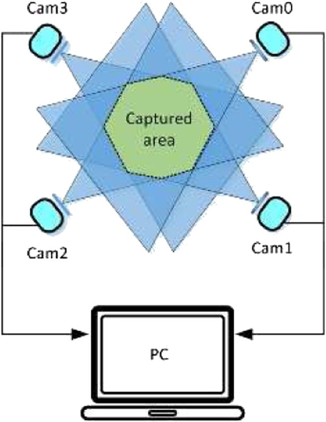
FIGURE 2 | Multi-view acquisition system architecture.
according to the natural connection of the human body. The
outputs of our model included not only the 3D mesh model of the
human but also the 3D coordinates of the joints. Therefore, under
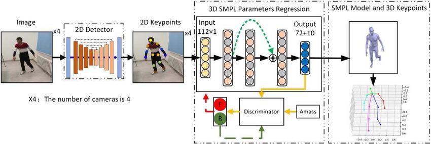
that predicted 3D pose from the 2D heatmap. They augmented a the premise of ensuring the accuracy of 3D human body
state-of-the-art 2D pose estimation structure to obtain a 2D estimation, real-time performance was also a factor that
heatmap. Tekin et al. [15] proposed novel two-branch needed to be considered. We specifically designed a fully
architecture with a trainable fusion scheme to fuse the 2D connected neural network with skip connections to estimate
heatmaps information optimally. There was an inverse for the the parameters of the SMPL model. The parameters of
human posture projected from a 2D feature map to 3D. To
resolve this problem, Li and Lee et al. [16] proposed a new
method to generate multiple feasible hypotheses of 3D posture
from 2D input that can choose the best solution from 2D
reprojections. Qammaz and Argyros [17] presented
MocapNET which offered a conquer-and-divide strategy to get
3D Bio Vision Hierarchical (BVH) [18] format. To tackle 3D
human pose estimation, Wang et al. [19] proposed a depth
ranking method (DRPose3D) that contains rich 3D
information. They estimated 3D pose from 2D joint locations
and depth rankings.
In the above algorithms, researchers only focused on the 3D
coordinates of joints, which were composed of dots and lines,
and showed no details about the human body shape and
appearance. Therefore, some researchers proposed a method
to predict the 3D human model from 2D images. Sigal et al. [20]
predicted the 3D human model by the outline shape of the body
in the image and adopted a shape completion and animation of
people [21] (SCAPE) to match the outline of the human body in
the image. Federica et al. [22] estimated a full 3D mesh model
FIGURE 3 | Position distribution of four cameras.
from a single image, called SMPLify. They estimated the 2D
Frontiers in Physics | www.frontiersin.org 3 February 2021 | Volume 9 | Article 629288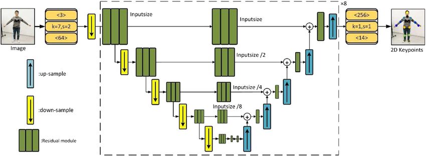
Meng and Gao                                                                                                               Human Pose Estimation

  FIGURE 4 | 3D human pose estimation structure.

  FIGURE 5 | Overall structure of the 2D stacked hourglass network.

proposed network model were much less than other state-of-the-                                        PT2 EP1  0,                             (1)
art algorithms.
                                                                           where E represents the essential matrix.
                                                                              Our method performs information fusion on images collected
METHODS                                                                    by four cameras at different positions in a certain activity space,
                                                                           and the implicit camera parameter relationship is learned
Multi-View Image Capture System                                            through a multilayer fully connected neural network.
Compared with the 2D plane, the dimension of spatial depth                 Therefore, our image acquisition system needs four optical
increases in the 3D space. Inspired by epipolar geometry, we note          sensors to acquire images of the experimenter in this certain
that images from multiple perspectives have some corresponding             activity space. The overall structure of the system is shown in
relations, which can reduce the ambiguity of projection. As shown          Figure 2. Four optical sensors are used for image acquisition. The
in Figure 1, C1 and C2 are the centers of the two cameras, e and e’        computer analyzes the image data through the algorithm we
are the epipoles, and the green plane area represents the epipolar         proposed to estimate the 3D human model and the position of 3D
plane. The point P1 means the joint in the image plane (gray box),         joint points.
which is projected into 3D space. The point P exists on a straight            The image acquisition instrument selects the industrial vision
line but the specific position is uncertain. The corresponding joint        inspection camera named Basler piA1000. This model of camera
is a point P2 in another view, and the intersection point of two           uses KAI-1020 CCD photosensitive chip, and the resolution is
projection lines can determine the position of the point P in the 3D       1,000 × 1,000, which meets the requirements of experimental data
space. Epipolar constraint is a significant property that can be            acquisition. The KAI-1020 CCD image sensor is a megapixel
written as                                                                 interline transfer CCD with an integrated clock driver and

Frontiers in Physics | www.frontiersin.org                             4                                  February 2021 | Volume 9 | Article 629288
Meng and Gao                                                                                                              Human Pose Estimation

  FIGURE 6 | Fully connected 3D parameters regression network.

associated on-chip double sampling, and the size of the                  simplest fully connected neural network with the SMPL model
photosensitive chip is 7.4 mm × 7.4 mm. The data                         to obtain the 3D human posture, as shown in Figure 4, which
transmission uses the GigE interface, and the data is                    consists of three stages:
transmitted to the computer directly without a frame grabber.
The camera has provided a set of basic preprocessing functions,          (1) The first stage is to estimate the 2D joint coordinates of the
such as debayering, anti-false color, sharpening enhancement,                human through the convolutional neural network. The
and denoising. Besides, the preprocessing function can greatly               images of four cameras with different angles are taken as
improve the brightness, detail, and sharpness of the image, while            inputs, and the Hourglass Network proposed by Newell et al.
reducing noise.                                                              [9] is used to estimate the multi-view 2D pose.
   To reduce the ambiguity in predicting the 3D posture of the           (2) In the second stage, we design a multi-layer cascaded fully
human from the 2D image, and to be able to effectively take a                connected neural network whose input is multi-view 2D joint
photo of the whole body of the experimenter, the four cameras are            coordinates and outputs are SMPL model pose and shape
placed on the same level and the same plane. The experimental                parameters. We classify joints according to the natural
system has an active area of 4000 mm × 3000 mm, as shown in                  connection characteristics and design discriminators to
Figure 3. The plane center of the active area is the origin of the           learn the implicit spatial prior information.
three-dimensional world coordinate system. In this coordinate            (3) In the third stage, the 3D human mesh model and human
system, the spatial positions (mm) of cameras were camera 0                  posture are calculated by the SMPL model parameters. The
(2,000, 1,500, 1,550), camera 1 (2,000, −1,500, 1,550), camera 2             3D human mesh model more specifically and vividly shows
(−2,000, 1,500, 1,550), and camera 3 (−2,000, −1,500, 1,550). In             the 3D human body.
the process of horizontal arrangement and vertical placement, a
certain direction allows error ±100 mm and ±50 mm,
respectively.                                                            2D Human Pose Detector
   For the multi-view acquisition system, it is crucial to acquire       At present, most convolutional neural networks adopt deeper
images synchronously. We set the time and date for multiple              layers, such as VGG-16 [29], Resnet-50, or Resnet-101 [30]. The
cameras using the Precision Time Protocol (PTP). According to            network of different depths can extract different levels of features.
time, the image is added timestamp. The operation instructions           The shallow network extracts local features, such as human head
are sent to multiple cameras to allow each camera to accurately          feature information or shoulder texture contours, which belong to
capture images at a predefined time point. Camera calibration is          low-level feature information. The features extracted by the deep
also an essential step in image acquisition using multi-view             network are global features, which are more comprehensive and
cameras. The geometric model is established through camera               abstract, such as the relative position relationship between
calibration, which is the object mapped from the 3D world to the         different parts of the human body. It is necessary to fuse the
imaging plane of the camera. In the process of camera calibration,       shallow features with deep features at the same time.
we used the Zhang–Calibration method. Through the chessboard                The input image size is 256 × 256 × 3. In the convolution
calibration board composed of black and white squares at                 operation block (orange box), the number above represents the
intervals and Pylon development software, we obtained the                number of input channels, the number below represents the
relevant parameters.                                                     number of output channels, k denotes the size of the convolution
                                                                         kernel, and s represents the step value. All downsampled blocks in
3D Human Pose Estimation Algorithm                                       the network use the maximum pooling operation, and upsampling
Our goal is to estimate the 3D human pose from the RGB images,           blocks use the nearest neighbor operation. The dotted line part in
where the 3D human pose includes the 3D joint point coordinates          Figure 5 is the hourglass basic model that can be expanded into
and the 3D human mesh model. Our method combines the                     cascades of multiple modules. The output of the network is the 2D

Frontiers in Physics | www.frontiersin.org                           5                                   February 2021 | Volume 9 | Article 629288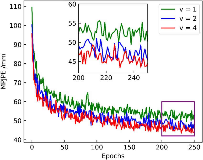
Meng and Gao                                                                                                                   Human Pose Estimation

                                                                                  The essence is to find a functional mapping relationship (F :
                                                                               R4×2×14 1R72+20 ). In this regression calculation, we adopt a
                                                                               simple and efficient fully connected neural network, thus
                                                                               greatly reducing the operation time while ensuring certain
                                                                               joint accuracy. Based on the above considerations, this paper
                                                                               designs a 3D human pose estimation neural network as shown in
                                                                               Figure 6, specifically as shown in Algorithm 1.
                                                                                  Algorithm 1 Fully connected neural network regressing SMPL
                                                                               parameters.
                                                                               The fully connected neural network we designed has six layers,
  FIGURE 7 | Prior knowledge network for adversarial learning in groups.       including an input layer, four intermediate layers, and an
                                                                               output layer. The selection of the number of layers is
                                                                               explained in detail in the Number of Fully Connected Layers
joint coordinates. Each green rectangle represents the residual                section. According to the characteristics of the fully connected
module in Figure 5. The residual connection is used to fuse the                network, the input data needs to be converted into a vector
extracted shallow features with the following deep features of the             before being sent to the 3D human posture regression network,
same size, and more robust joint positions are obtained by using the           so the input data is 112 dimensions. The output layer reduces
information of spatial position distribution between joints.                   to 82-dimensional SMPL model parameters. The hidden layers
    The network module structure is symmetrical and similar to                 (FC2, FC3, FC4, and FC5) use the same number of neurons.
the shape of an hourglass, so it is called the stacked hourglass               The network uses 2,048 neurons for network learning. The
network. The input images from the four angles of view are used                selection of this parameter is analyzed in the The Number of
to extract the joint point features through the stacked hourglass              Neurons section.At the same time, to achieve the fusion of
network, and the joint point coordinates of the human body are                 feature information between different layers, every two layers
calculated. The above is the main content of the first stage of the             use skip connection. Skip connection is to merge the input
algorithm model in this paper. According to the analysis of the                information of the front layer with the output information of
Numbers of Hourglass Network Modules section, the number of                    the back layer network and send it to the next fully connected
hourglass basic modules in this paper is finally set to 8.                      layer, as shown in Figure 6. The skip connection is denoted as

Fully Connected 3D Parameters Regression Network                                                             H(x)  F(x) + x.               (2)
At this stage, our goal is to learn the mapping relationship                   Even if skip connections are added to the neural network, the
between the 2D joint coordinates and the pose and shape                        efficiency is not affected, because it is very easy to learn the
parameters of the SMPL model. To learn this mapping                            identity function for a fully connected network. The addition of
relationship, this paper specially designs a multi-level fully                 skip connections not only improves the performance of the
connected neural network. The input data is the 2D joint                       network but also reduces the possibility of gradient
coordinates X ∈ R4×2×N from the four cameras (in this paper,                   disappearance during training. In our method, because the
14 joint points are taken, so N  14). The output of the network               number of neurons in each hidden layer is the same, direct
is the shape and pose parameters of the SMPL mesh model                        skip connections can be used, and there is no need to change
(where shape parameters are β ∈ R10 , and pose parameters                      the dimension of the feature information. The whole network
are θ ∈ R72 ).                                                                 completes the regression from 2D joint to 3D human parameters,
    We use the SMPL model, introduced by Loper et al. [24], due                and the network is simpler and lighter. Compared with the
to their low-dimensional parameter space, compared to voxelized                convolutional neural network, the fully connected neural
or point cloud representations, which is very suitable for direct              network can integrate the local features of the previous layer
network prediction. We describe the SMPL body model and                        to obtain the global features and obtain more abstract features.
provide the essential notation here. For more details, you can read
this paper [24]. The SMPL model is a parametric human body                     Learnable Adversarial Prior
mode, so the parameters of the human are divided into pose                     The human joints have high flexibility, and various actions and
parameters θ ∈ R72 and shape parameters β ∈ R10 . The shape                    postures are produced in 3D space, which brings great challenges
parameters are the linear coefficients of a 10-dimension shape                  to the prediction of the spatial position of joints. However, the
space, which reduce to low-dimensional by principal component                  skeletal structure of the human has strict symmetry and a certain
analysis (PCA). The different shape parameters show the height,                limited position of the relative hinge motion between the human
weight, body proportion, and body shape of people with various                 joints. Therefore, there are some prior constraints between the
body types. The pose parameters θ denote the axis-angle                        joints, such as the bone ratio and the limit of the rotation angle
representation (θi ∈ R3 ) of the relative rotation between parts               between the joint points.
in the 3D space. The pose parameters (θ ∈ R23×3+3 , 3 for each of                 Inspired by the idea of generating adversarial networks (GAN)
the 23 joints, plus 3 for the global rotation) consist of the root             [31], we adopt a data-driven approach to learn the implicit prior
orientation and 23 joints which are defined by a skeleton rig.                  information of the spatial structure of human joint points. Unlike
                                                                               directly providing the model with fixed joint point prior

Frontiers in Physics | www.frontiersin.org                                 6                                  February 2021 | Volume 9 | Article 629288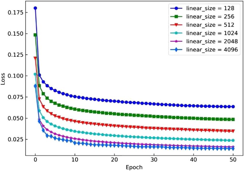
Meng and Gao                                                                                                                                   Human Pose Estimation

TABLE 1 | Comparative results of MPJPE for predicting 3D joints under Protocol #1. The best score is marked in bold.

Protocol          Direc     Disc      Eat     Greet   Phon     Photo     Pos        Pur        Sit     SitD     Smok      Wait     WalkD      Walk     WalkT     AVG
#1

Zhou [14]         54.8      60.7     58.2     71.4     62.0    65.5      53.8    55.6         75.2    111.6      64.2     66.1      51.4      63.2      55.3     64.9
Fang [41]         50.1      54.3     57.0     57.1     66.6    73.3      53.4    55.7         72.8     88.6      60.3     57.7      62.7      47.5      50.6     60.4
Sun [42]          52.8      54.8     54.2     54.3     61.8    67..2     53.1    53.6         71.7     86.7      61.5     53.4      61.6      47.1      53.4     59.1
Yang [43]         51.5      58.9     50.4     57.0     62.1    65.4      49.8    52.7         69.2     85.2      57.4     58.4      43.6      60.1      47.7     58.6
Pavlakos [44]     41.2      49.2     42.8     43.4     55.6    46.9      40.3    63.7         97.6    119.9      52.1     42.7      51.9      41.8      39.4     56.9
Pavlakos [8]      48.5      54.4     54.4     52.0     59.4    65.3      49.9    52.9         65.8     71.1      56.6     52.9      60.9      44.7      47.8     56.2
Ci [45]           46.8      52.3     44.7     50.4     52.9    68.9      49.6    46.4         60.2     78.9      51.2     50.0      54.8      40.4      43.3     52.7
Li [16]           46.8      52.3     44.7     50.4     52.9    68.9      49.6    46.4         60.2     78.9      51.2     50.0      54.8      40.4      43.3     52.7
Xiao [46]         46.5      48.1     49.9     51.1     47.3    43.2      45.9    57.0         77.6     47.9      54.9     46.9      37.1      49.8      41.2     49.8
Cai [47]          44.6      47.4     45.6     48.8     50.8    59.0      47.2    43.9         57.9     61.9      49.7     46.6      51.3      37.1      39.4     48.8
Ours (V1)         44.6      52.2     43.9     52.8     51.0    71.6      47.1    44.9         61.6     64.6      54.4     51.1      61.4      48.8      54.0     53.6
Ours (V2)         37.6      46.4     41.7     46.2     51.7    62.9      43.8    45.2         60.7     57.1      55.6     44.4      52.9      44.8      48.8     49.3
Ours (V4)         36.8      44.8     41.3     44.3     46.1    59.3      42.2    42.1         53.2     56.1      50.9     44.0      53.0      44.6      47.2     47.1

TABLE 2 | Results showing the PA-MPJPE on Human3.6M under Protocol #2. The best score is marked in bold.

Protocol        Direc     Disc      Eat      Greet    Phon    Photo     Pos      Pur          Sit     SitD     Smok      Wait     WalkD      Walk      WalkT     AVG
#2

Chen [48]       36.9      39.3     40.5      41.2     42.0     34.9     38.0     51.2        67.5     42.1      42.5     37.5       30.6      40.2      34.2     41.6
Cai [47]        35.7      37.8     36.9      40.7     39.6     45.2     37.4     34.5        46.9     50.1      40.5     36.1       41.0      29.6      33.2     39.0
Pavllo [49]     34.1      36.1     34.4      37.2     36.4     42.2     34.4     33.6        45.0     52.5      39.6     35.4       39.4      27.3      28.6     38.1
Dabral [50]     28.0      30.7     39.1      34.4     37.1     28.9     31.2     39.3        60.6     39.3      44.8     31.1       25.3      37.8      28.4     36.3
Wang [51]       28.4      32.5     34.4      32.3     32.5     40.9     30.4     29.3        42.6     45.2      33.0     32.0       33.2      24.2      22.9     32.7
Ours (V1)       34.5      35.5     35.5      37.1     40.1     45.5     31.9     34.7        48.5     46.4      40.5     35.6       39.4      33.6      37.6     38.6
Ours (V2)       25.1      32.9     25.3      30.6     35.6     39.9     26.5     26.5        34.7     36.4      32.8     29.2       33.6      27.8      31.0     31.9
Ours (V4)       24.3      30.1     25.4      29.9     33.9     38.6     26.7     26.1        34.5     36.1      31.6     28.9       33.9      27.8      29.4     30.5

constraints [32–35], our method continues to learnable and
flexible, which improves the generalization ability of the
model. Besides, we also group the joints of the human
according to the correlation between the joints of the human
body. For a group of joints with a strong correlation, the same
simple discriminant neural network is used.
   Due to the relative hinge movement of human joints, it is
natural for us to think that the position information of some
joints provides important reference information and geometric
constraints for the positioning of other joints, such as between the
knee and the ankle. However, due to the high flexibility of the
human body, not all joints are very close, such as the wrist and
ankle. Based on the natural connection between human
structures and the correlation between joints [36, 37], we
classify the joint points of the human body. The joint points
related to this paper are divided into six classes: 1) head and neck;
2) left wrist, left elbow, and left shoulder; 3) right wrist, right
elbow, and right shoulder; 4) left knee and left ankle; 5) right knee
and right ankle; 6) left hip and right hip.                                               FIGURE 8 | MPJPE curve under different number of perspectives in the
                                                                                          training.
   We design a set of human 3D pose discriminators (D1, D2,
etc.) to distinguish the pose and shape parameters of the human
body predicted by the previously fully connected neural network                      abnormal body shape (such as abnormal thick or abnormal small
and determine whether it is a real human body. A learnable                           joints), we designed a shape discriminator. At the same time, to
discriminator is designed for each group of joints to learn the                      learn the joint prior knowledge of all parameters, we also designed
distribution of normal human joint position data, thus reducing                      a discriminator for all parameters of the human body
the generation of exaggerated data. To reduce the possibility of                     parameterized by SMPL. Therefore, we design eight

Frontiers in Physics | www.frontiersin.org                                      7                                            February 2021 | Volume 9 | Article 629288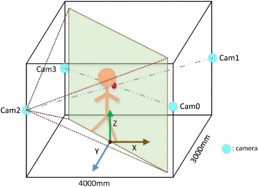
Meng and Gao                                                                                                                  Human Pose Estimation

                                                                         operating system of Linux and the CPU model of Intel Core i5-
                                                                         7500 CPU @3.40 GHz.

                                                                         Implementation Details
                                                                         In the stacked hourglass network for detecting the 2D joint
                                                                         coordinates, the number of hourglass modules was 8, the
                                                                         learning rate was set to 1 × 10⁻⁴, and the batch-size was set to
                                                                         16, and the network had undergone 50,000 iterative training
                                                                         processes. The regressed network learned the mapping
                                                                         relationship between the 2D joint coordinates and the parameters
                                                                         of the SMPL model. The Adam optimizer was used, the learning rate
                                                                         was set to 0.001, the exponential decay optimization method was
                                                                         used, and the batch size was set to 64, with 250 epochs.

                                                                         Experiment on 3D Pose of Human3.6M
                                                                         To compare with other state-of-the-art human pose estimation
                                                                         methods, we conduct experimental evaluations of the proposed
                                                                         method on the public 3D human pose estimation dataset Human
                                                                         3.6M [39], which consists of 3.6 million images and collects 15
                                                                         daily activities performed by 11 experimenters under four camera
                                                                         views. To facilitate the evaluation and recording of the
                                                                         experimental results, each action in the dataset was marked
  FIGURE 9 | Accuracy of different numbers of hourglass network          with abbreviations, for example, Directions as Direc,
  modules on evaluation.
                                                                         Discussion as Disc, Eating as Eat, Greeting as Greet, and so on.
                                                                             We follow the standard protocols to evaluate our approach.
                                                                         Images of subjects S1, S5, S6, and S7 are used for model training,
discriminators in this article. Finally, the average value of the        and S9 and S11 are used for testing. Protocol #1 is the Mean Per
discriminators is calculated as the final discrimination result.          Joint Position Error (MPJPE, millimeter) between the ground-truth
    As shown in Figure 7, the fully connected neural network             and the prediction. In some works, the predicted 3D pose is firstly
serves as a generator (G) to generate the pose and shape                 aligned with a rigid transformation using Procrustes Analysis [40]
parameters of the 3D human G(θ, β) ∈ R82 . Amass is a large-             and then compute the Mean Per Joint Position Error (PA-MPJPE),
scale human 3D motion dataset. We select the corresponding               which is called Protocol #2. The MPJPE is denoted as
parameters in the Amass dataset [38] as the real data
R(θ, β) ∈ R82 . These two sets of data are fed into                                                    1 N
                                                                                           MPJPE         Hpre (i) − Hgt (i),                   (3)
discriminators (D1, D2, etc.) to judge whether the SMPL                                                N i1
parameters generated by the fully connected neural network
conform to the real human body parameter data distribution.
Through adversarial training, we learn the implicit prior
knowledge of the spatial structure of key human nodes, so
that the results generated by the fully connected network are
more in line with the shape of the real human body.
    Considering that the task of the discriminator is a simple
binary classification, our discriminators (D) also adopt a simple
fully connected neural network. Since the number of joints in
each group is different, the dimensions of the input layer of each
discriminator are different, and the output layer is the result of
judging whether the input parameters conform to the distribution
of real human body data. The middle two hidden layers of the
network use 1,024 neurons for training to learn the real
distribution of joint rotation vectors in the same group.

EXPERIMENTS
Experimental Equipment
The training and testing of the experimental model in this article
                                                                          FIGURE 10 | Training loss curve of 3D pose regression network.
are completed on the NVIDIA GeForce RTX 2070, with the

Frontiers in Physics | www.frontiersin.org                           8                                      February 2021 | Volume 9 | Article 629288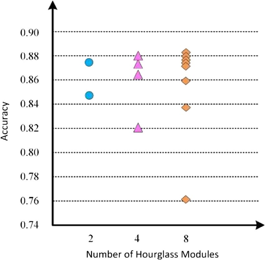
Meng and Gao                                                                                                                Human Pose Estimation

                                                                            depth blur problem and made up for the inaccurate
                                                                            detection of the 2D joint detector.
                                                                               Compared with other methods, we not only calculated the 3D
                                                                            space position of the human body joint points but also estimated
                                                                            the 3D mesh model of the human body. Our representation
                                                                            method was more vivid and lifelike than the representation of the
                                                                            line between the joint points, so the method in this paper was
                                                                            better than other algorithms in the overall prediction effect.

                                                                            Running Time
                                                                            To test the running time of the proposed algorithm in the 3D
                                                                            human pose estimation, it was compared with Simplify and HMR
                                                                            under the same experimental conditions (see the Experimental
                                                                            Equipment section). Table 3 summarizes the results from the
  FIGURE 11 | Model training time comparison.                               different algorithms. The average time per frame of Simplify [22]
                                                                            algorithm was 199.2 s. The reason was that the model was based
                                                                            on the parameter optimization method to match the SMPL model
where N represents the number of joints of the human, Hpre (i)              with 2D joint points, and the optimization process took a lot of
represents the predicted position at the ith joint point, and               time. HMR [52] algorithm needed 7.8 s per frame, and the model
similarly Hgt (i) represents the ground-truth of the ith joint point.       obtains the parameters of the 3D human model from the images
   We compared the results with those achieved in the past three            by iterative regression, which improved the operational efficiency
years and conducted quantitative comparisons of the two                     to a certain extent. The proposed algorithm is 1.3 s per frame,
standard protocols in Tables 1 and 2, respectively. The best                where the average cost was 75 ms for the 2D human pose
score is marked in bold. We performed three sets of tests on the            estimation and 1.225 s for the 3D SMPL model parameter
number of different cameras. V1, V2, and V4 represent images                estimation and 3D human mesh model rendering, which took
from 1, 2, and 4 viewing angles, respectively. The results showed           a large part of the time. Therefore, the fully connected network
that our method outperforms other methods in all evaluation                 structure proposed in this paper saved a large amount of model
protocols.                                                                  calculation time, improved the accuracy, and maintained high
   From the experimental results in Tables 1 and 2, it can be               efficiency.
seen that the overall ranking of this method was the first, and all
the sub-items were in the top three, and the overall error                  Ablation Experiment
calculated by the model was small. The method proposed by                   Considering that there are a large number of parameters that can
Cai et al. [47] used the spatial-temporal information to obtain             be optimized in the network structure designed in this paper, the
the spatial prior knowledge between joints, and the effect was              use of different parameter settings will have different effects on
superior to other algorithms. The method we proposed was to                 the accuracy and operation efficiency of the model, so we analyze
group the joints with strong correlation, and the designed                  the ablation experiments with different parameter configurations.
antagonistic prior knowledge module was used for each
group of joints to learn the spatial prior knowledge between                Numbers of Hourglass Network Modules
joint points, thus reducing the generation of exaggerated data.             The model estimation effect was different for different numbers
The effect was better, MPJPE was reduced from 48.8 to 47.1 mm,              of hourglass modules. To determine the effect of the number of
and PA-MPJPE was reduced by 8.5 mm.                                         hourglass modules on model accuracy, we compared the
   For the problem of depth ambiguity, Li et al. [16] introduced            performance of the 2D human pose estimation model on the
the mixture density model into 3D human pose estimation to                  test set, when different numbers of modules are used, and showed
solve the problem of projecting multiple feasible solutions. We             the changing process of the model estimation effected by
used images from multiple perspectives as input to solve the                calculating the accuracy of each hourglass module in Figure 9.
multi-solution problem and reduce the ambiguity of projection                  The abscissa represented the number of hourglass modules,
from 2D to 3D. The experimental analysis was performed with                 and the ordinate represented the accuracy of the corresponding
images from 1, 2, and 4 viewing angles as input (V1, V2, and V4).           different numbers of hourglass modules on the verification set.
In Tables 1 and 2, MPJPE and PA-MPJPE were reduced from                     Each column icon in the figure corresponded to a situation. For
53.6 to 47.1 mm and from 38.6 to 30.5 mm, respectively.                     example, the horizontal axis 2 indicated that the number of
   Figure 8 showed the changing process of MPJPE in our                     hourglass modules was 2, and there were two icons in the
training process by using images with different visual angles as            column, which, respectively, indicated the estimation accuracy
input. The horizontal axis represented the number of training               of the first and second hourglass modules in the model from
epochs, and the vertical axis represented MPJPE. We                         bottom to top, and so on.
discovered that, with the increase in the number of input                      Through comparison, it was found that, with the increase in
views, our method worked better. This was because the                       the number of hourglass modules, the accuracy rate was gradually
image information from multiple views can well solve the                    improved. The highest accuracy of hourglass module numbers 2,

Frontiers in Physics | www.frontiersin.org                              9                                  February 2021 | Volume 9 | Article 629288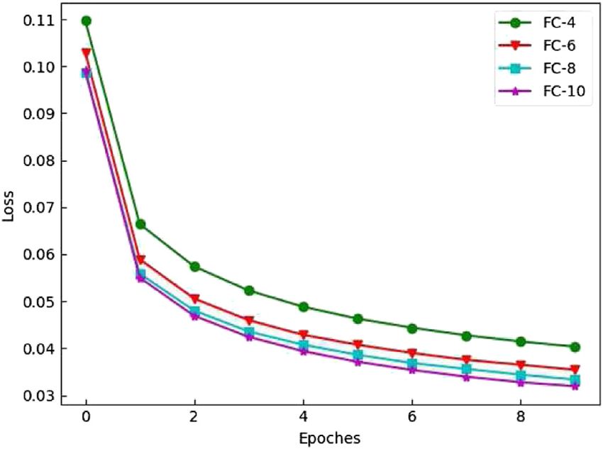
Meng and Gao                                                                                                                          Human Pose Estimation

                                                                              TABLE 3 | Running time comparison of 3D human mesh model estimation
                                                                              algorithm.

                                                                              Methods                                                          Average
                                                                                                                                            running time (s)

                                                                              Simplify [22]                                                       199.2
                                                                              HMR [52]                                                             7.8
                                                                              Ours                                                                 1.3

                                                                              TABLE 4 | MPJPE index experimental results for each joint of two experimenters
                                                                              (1, 2).

                                                                                                            Experimenter 1                   Experimenter 2

                                                                              Right ankle                        58.37                            59.87
                                                                              Right knee                         44.40                            34.76
  FIGURE 12 | Loss curves of different numbers of neurons.                    Right hip                           9.36                             9.45
                                                                              Left hip                            9.36                             9.45
                                                                              Left knee                          42.95                            39.28
                                                                              Left ankle                         75.22                            94.80
                                                                              Right wrist                        60.90                            59.09
                                                                              Right elbow                        52.19                            50.48
                                                                              Right shoulder                     46.66                            46.01
                                                                              Left shoulder                      51.77                            54.55
                                                                              Left elbow                         55.67                            64.88
                                                                              Left wrist                         66.20                            70.75
                                                                              Neck                               42.73                            39.26
                                                                              Head top                           55.80                            59.05
                                                                              AVG                                47.98                            49.40

                                                                              the model converged faster. It can be seen from the curve that the
                                                                              convergence speed of the model had little difference when the
                                                                              number of fully connected layers was 6, 8, and 10, and the number
                                                                              of parameters of the model was relatively less when the number of
                                                                              fully connected layers was 6.
                                                                                  For further illustration of the training process’s efficiency, we
  FIGURE 13 | Average joint error of different neuron numbers (mm).           conducted a statistical analysis of the training time of different
                                                                              numbers of fully connected layer models, as shown in Figure 11.
                                                                              As the number of fully connected layers increased, the time
4, and 8 is 0.875, 0.880, and 0.884, respectively. It can be seen that        consumed by the model also increased. Comprehensive
the larger the number of hourglass modules, the better the model              analysis of the results, We considered that the number of fully
estimation effect. However, with the deepening of the network                 connected layers was set to 6.
layer, the number of model parameters increases, and the
gradient easily disappears. Moreover, the variation amplitude                 The Number of Neurons
of the accuracy of model estimation decreased and tended to a                 In this paper, the 3D pose estimation was implemented using a
stable state. Therefore, the algorithm in this paper set the number           fully connected network, and the number of neurons in the fully
of hourglass modules to 8.                                                    connected layer had a certain impact on the number of model
                                                                              parameters and the prediction effect. Therefore, a comparative
Number of Fully Connected Layers                                              analysis is performed on networks with different numbers of
We analyzed the effect of choosing a different number of fully                neurons (Linear_size, which represents the number of neurons in
connected layers on the algorithm in the training process through             the fully connected layer).
experiments. In the experiment, we set the training process as 10                 To compare the effect of different neuron numbers on the
epochs in total, and the number of fully connected layers was set             model performance, we selected several classic parameter values
to 4 (FC-4), 6 (FC-6), 8 (FC-8), and 10 (FC-10). It can be seen that          128, 256, 512, 1,024, 2,048, 4,096 for experiments. As shown in
as the number of fully connected layers increases, the loss value of          Figure 12, The horizontal axis represented the number of epochs
the model decreases gradually and tended to convergence from                  of model training (we selected the first 50 epochs for analysis),
Figure 10. When the number of fully connected layers was larger,              and the vertical axis represented the loss function value of the

Frontiers in Physics | www.frontiersin.org                               10                                        February 2021 | Volume 9 | Article 629288
Meng and Gao Human Pose Estimation
measures were added to the network. It can be seen that the
loss function (Loss) value of model training was the highest.
When only Dropout and Residual were added to the network, the
green curve which was in the second place in the corresponding
figure shows a significant reduction in the loss value compared
with the case without optimization. When only Batch
Normalization (BN) layer and Dropout operations were added
to the network, corresponding to the light blue curve in the third
place in the figure, it can be seen that the loss had dropped more
significantly, which showed that the batch normalization affects
the loss value. The effect was remarkable. The curves in the fourth
and fifth places corresponded to the cases where the BN,
Dropout, and Residual optimization methods are added at
the same time, and the BN and Residual optimization
methods were added only. Through comparison, it was
found that the red curve had the lowest value. The network
model without Dropout will have higher prediction results for the
FIGURE 14 | Comparison of loss curves by using different methods. batch of training data, but the prediction effect of the model on the
new test data is often unsatisfactory. Because Dropout operations
were used to solve the over-fitting problem of the model, the
training process. We can observe that when the number of parameters of model training will be biased toward overfitting, so
neurons increases from 128 to 4,096, the loss value gradually the loss value will be relatively low. This is disadvantageous for
declines. It indicated that the accuracy of model training was our model.
approximately positively correlated with the number of neurons; Based on the above curve analysis, BN improved the
that is, the higher the number of neurons is, the higher the prediction effect of the network, and the extracted feature
accuracy of model estimation will be. information was fused by the skip connection method.
To determine the effect of the number of neurons on the Compared with the model without the Dropout method, the
model performance better, we further conducted comparative smallest loss was obtained. But considering the generalization
experiments on the network prediction effects with different ability of the model, it was necessary to finally choose to add the
numbers of neurons. The 50 batches of test images were Dropout layer.
randomly selected to verify the model prediction effect. The
number of images in each batch was 64, and 3,200 images were Experiment of Multi-View Capturing Images
used for this experiment. The abscissa represented the number The capturing system was used for image acquisition. The
of neurons in each layer, the parameters were set to 128, 512, experimental subjects moved in the active area and did some
1,024, 2,048, and 4,096, and the ordinate represented the actions in daily life, to ensure that the experimental subjects were
MPJPE (mm) of the joint errors in Figure 13. By comparing located in the perspective of the camera as far as possible. The
the prediction results of different numbers of neurons, it was stacked hourglass convolutional network was used as the 2D
found that the error value of 4,096 neurons was only 0.3 mm detector to detect the 2D joint point of the image under four
lower than the error value of 2,048 neurons. This indicated that perspectives (X, Y ∈ R4×14×2 ). The 2D coordinates were input
the prediction effects of the two models were not much into the fully connected neural network designed in this paper,
different. Compared with the model with 4,096 neurons, the and the parameters of the SMPL model were obtained by
model with 2,048 neurons had fewer parameters. Considering regression calculation (θ, β ∈ R82 ). The 3D human mesh
comprehensively, this article set the number of neurons in the model was obtained through the SMPL model, and the 3D
fully connected layer to 2,048. joint point coordinates of the human body were further
calculated. Using this experimental system, experimenter 1 and
Optimization Method experimenter 2 were tested with 5,000 images, and the test results
To make the fully connected network better learn the mapping were quantitatively analyzed by quantitative index MPJPE. The
relationship between 2D joint points and 3D model parameters, analysis results were shown in Table 4.
we added optimization methods such as batch normalization, The joints such as the right ankle, left ankle, right hand, and
dropout, and skip connection between layers. For whether these left wrist had higher error values than other joint points. The
optimization methods had a positive impact on the model, and reason was that these joint points of the human body were
how to choose the best combination plan, we further conducted flexible, and the ankle joints were easy to be occluded
experiments and analysis. compared with other joints, so the error of the model in
The abscissa represented the number of epochs of model estimating the position of these joint points was larger. To
training, and the ordinate indicated the value of the loss improve the accuracy of model prediction, the next step is to
function during the training process, shown in Figure 14. The focus on improving the prediction accuracy of these easily
purple-red curve at the top indicated that no optimization occluded joints and joints with greater flexibility, which should
Frontiers in Physics | www.frontiersin.org 11 February 2021 | Volume 9 | Article 629288Meng and Gao Human Pose Estimation
be constrained by the symmetry of the human structure and the DATA AVAILABILITY STATEMENT
proportion of the joints, thus reducing the error in the estimation
of joint point coordinates. The original contributions presented in the study are included in
the article/Supplementary Material. Further inquiries can be
directed to the corresponding author.
CONCLUSION
We proposed a multi-layer fully connected neural network
with skip connections to learn the mapping relationship ETHICS STATEMENT
between the 2D joint coordinates and the parameters of
Written informed consent was obtained from the individuals for
the SMPL model. we classified joints according to the
the publication of any potentially identifiable images or data
natural connection characteristics and used a data-driven
included in this article.
method to learn the implicit spatial prior information.
Besides, we constructed a multi-view image acquisition
system. The experimenter performs some daily behavioral AUTHOR CONTRIBUTIONS
activities in a certain activity space. We used four optical
sensors to collect images of the experimenter, and the LM is the main contributor of this work, and Hengshang Gao
computer analyzed the image via the algorithm we focused on the experimental design and debug.
proposed to estimate the 3D human mesh model and the
3D joint locations. The experimental results showed that the
MPJPE of the 3D human pose estimated by the algorithm in FUNDING
this paper was the smallest, and it ranked first among all the
algorithms participating in the comparison. The future work This research was funded by National Key Research and
is to analyze multi-frame video sequences and restore the Development Project (2018YFB2003203), National Natural
distortion of postures by studying the continuity information Science Foundation of China (62073061), and Fundamental
of postures. Research Funds for the Central Universities (N2004020).
10. Wei S, Ramakrishna V, Kanade T, Sheikh Y. Convolutional pose machine. In:
REFERENCES IEEE conference on computer vision and pattern recognition (2016) p.
4724–32. doi:10.1109/CVPR.2016.511
1. Yang F, Sakti S, Wu Y, Nakamura S. Make skeleton-based action recognition 11. Zhou X, Zhu M, Leonardos S, Derpanis KG, Daniilidis K. Sparseness meets
model smaller, faster and better. In: Proceedings of the ACM multimedia asia deepness: 3D human pose estimation from monocular video. In: IEEE
(2019) p. 1–6. doi:10.1145/3338533.3366569 conference on computer vision and pattern recognition (2016) p. 4966–75.
2. Liu J, Wang G, Duan LY, Abdiyeva K, Kot AC. Skeleton-based human doi:10.1109/CVPR.2016.537
action recognition with global context-aware attention LSTM networks. 12. Martinez J, Hossain R, Romero J, Little JJ. A simple yet effective baseline for 3d
IEEE Trans Image Process (2018) 27(4):1586–99 doi:10.1109/TIP.2017. human pose estimation. In: IEEE international conference on computer vision
2785279 (2017) p. 2640–9. doi:10.1109/ICCV.2017.288
3. Shi L, Zhang Y, Cheng J, Lu H. Skeleton-based action recognition with multi- 13. Ramakrishna V, Kanade T, Sheikh Y. Reconstructing 3D human pose from 2D
stream adaptive graph convolutional networks. IEEE Trans Image Process image landmarks. In: European conference on computer vision (2012) p.
(2020) 29:9532–45 doi:10.1109/TIP.2020.3028207 573–86. doi:10.1007/978-3-642-33765-9_41
4. Li M, Chen S, Chen X, Zhang Y, Wang Y, Tian Q. Actional-structural graph 14. Zhou X, Huang Q, Sun X, Xue X, Wei Y. Towards 3D human pose estimation
convolutional networks for skeleton-based action recognition. In: Proceedings in the wild: a weakly-supervised approach. In: IEEE international conference
of the IEEE conference on computer vision and pattern recognition (2019) on computer vision (2017) p. 398–407. doi:10.1109/ICCV.2017.51
p. 3590–8. doi:10.1109/CVPR.2019.00371 15. Tekin B, Márquez-Neila P, Salzmann M, Fua P. Learning to fuse 2D and 3D
5. Su K, Liu X, Shlizerman E. Predict & cluster: unsupervised skeleton based image cues for monocular body pose estimation. In: IEEE international
action recognition. In: Proceedings of the IEEE conference on computer conference on computer vision (2017) p. 3941–50. doi:10.1109/ICCV.2017.42
vision and pattern recognition (2020) p. 13–9. doi:10.1109/CVPR42600.2020. 16. Li C, Lee GH. Generating multiple hypotheses for 3D human pose estimation
00965 with mixture density network. In: IEEE conference on computer vision and
6. Rogez G, Weinzaepfel P, Schmid C. LCR-net: localization-classification-regression pattern recognition (2019) p. 9887–95. doi:10.1109/CVPR.2019.01012
for human pose. In: Proceedings of the IEEE conference on computer vision and 17. Qammaz A, Argyros A. MocapNET: ensemble of SNN encoders for 3D human pose
pattern recognition (2017) p. 21–6. doi:10.1109/CVPR.2017.134 estimation in RGB images. In: British machine vision conference (2019) p. 46–63.
7. Pavlakos G, Zhou X, Derpanis KG, Daniilidis K. Coarse-to-Fine volumetric 18. Meredith M, Maddock SC. Motion capture file formats explained. Dep Comput
prediction for single-image 3D human pose. In: Proceedings of the IEEE Sci (2001) 211:241–4
conference on computer vision and pattern recognition (2017) p. 21–6. 19. Wang M, Chen X, Liu W, Qian C, Lin L, Ma L. DRPose3D: depth ranking in
doi:10.1109/CVPR.2017.139 3D human pose estimation. In: Twenty-Seventh international joint conference
8. Pavlakos G, Zhou X, Daniilidis K. Ordinal depth supervision for 3D human on artificial intelligence (2018) p. 1805. doi:10.24963/ijcai.2018/136
pose estimation. In: Proceedings of the IEEE Conference on Computer 20. Sigal L, Balan A, Black MJ. Combined discriminative and generative articulated pose
Vision and Pattern Recognition (2018) p. 7307–16. doi:10.1109/CVPR. and non-rigid shape estimation. Adv Neural Inf Process Syst (2007) 25:1337–44
2018.00763 21. Anguelov D, Srinivasan P, Koller D, Thrun S, Rodgers J, Davis J. Scape. ACM
9. Newell A, Yang K, Deng J. Stacked hourglass networks for human pose Trans Graph (2005) 24(3):408–16 doi:10.1145/1073204.1073207
estimation. In: Proceedings of the European conference on computer vision 22. Bogo F, Kanazawa A, Lassner C, Gehler P, Romero J, Black MJ. Keep it SMPL:
(2016) p. 483–99. doi:10.1007/978-3-319-46484-8_29 automatic estimation of 3D human pose and shape from a single image. In:
Frontiers in Physics | www.frontiersin.org 12 February 2021 | Volume 9 | Article 629288Meng and Gao Human Pose Estimation
European conference on computer vision (2016) p. 561–78. doi:10.1007/978- 39. Ionescu C, Papava D, Olaru V, Sminchisescu C. Human3.6M: large scale
3-319-46454-1_34 datasets and predictive methods for 3D human sensing in natural
23. Pishchulin L, Insafutdinov E, Tang S, Andres B, Andriluka M, Gehler P, et al. environments. IEEE Trans Pattern Anal Mach Intell (2014) 36(7):1325–39
DeepCut: joint subset partition and labeling for multi person pose estimation. doi:10.1109/TPAMI.2013.248
In: IEEE conference on computer vision and pattern recognition (2016) p. 40. Gower JC Generalized procrustes analysis. Psychometrika (1975) 40(1):33–51
4929–37. doi:10.1109/CVPR.2016.533 doi:10.1007/BF02291478
24. Loper M, Mahmood N, Romero J, Pons-Moll G, Black MJ. SMPL. ACM Trans 41. Fang H, Xu Y, Wang W, Liu X, Zhu S. Learning pose grammar to encode human
Graph (2015) 34(6):1–16 doi:10.1145/2816795.2818013 body configuration for 3D pose estimation. In: Proceedings of the AAAI (2018)
25. Lassner C, Romero J, Kiefel M, Bogo F, Black MJ, Gehler PV. Unite the people: 42. Sun X, Shang J, Liang S, Wei Y. Compositional human pose regression. In:
closing the loop between 3D and 2D human representations. In: IEEE IEEE international conference on computer vision (2017) p. 2602–11. doi:10.
conference on computer vision and pattern recognition (2017) p. 6050–9. 1109/ICCV.2017.284
doi:10.1109/CVPR.2017.500 43. Yang W, Ouyang W, Wang X, Ren J, Li H, Wang X. 3D human pose estimation
26. Güler RA, Neverova N, Kokkinos I. DensePose: dense human pose estimation in the wild by adversarial learning. In: IEEE conference on computer vision
in the wild. In: IEEE conference on computer vision and pattern recognition and pattern recognition (2018) p. 5255–64. doi:10.1109/CVPR.2018.00551
(2018) p. 7297–306. doi:10.1109/CVPR.2018.00762 44. Pavlakos G, Zhou X, Derpanis K, Daniilidis K. Harvesting multiple views for
27. Yao P, Fang Z, Wu F, Feng Y, Li J. DenseBody: directly regressing dense 3D marker-less 3D human pose annotations. In: IEEE conference on computer
human pose and shape from a single color image. arXiv [Preprint] (2019) vision and pattern recognition (2017) p. 6988–97. doi:10.1109/CVPR.2017.138
Available from: arXiv:1903.10153. 45. Ci H, Wang C, Ma X, Wang Y. Optimizing network structure for 3D human
28. Kocabas M, Athanasiou N, Black MJ. VIBE: video inference for human pose estimation. In: IEEE international conference on computer vision (2019)
body pose and shape estimation. In: IEEE conference on computer vision p. 2262–71. doi:10.1109/ICCV.2019.00235
and pattern recognition (2020) p. 5253–63. doi:10.1109/CVPR42600.2020. 46. Sun X, Xiao B, Wei F, Liang S, Wei Y. Integral human pose regression. In:
00530 Proceedings of the European conference on computer vision (2018) p. 536–53.
29. Simonyan K, Zisserman A. Very deep convolutional networks for large- doi:10.1007/978-3-030-01231-1_33
scale image recognition. arXiv [Preprint] (2014) Available from: arXiv: 47. Cai Y, Ge L, Liu J, Cai J, Cham T-J, Yuan J, et al. Exploiting spatial-temporal
1409.1556. relationships for 3D pose estimation via graph convolutional networks. In:
30. He K, Zhang X, Ren S, Sun J. Deep residual learning for image recognition. In: International conference on computer vision (2019) p. 227–2281. doi:10.1109/
Proceedings of the IEEE conference on computer vision and pattern ICCV.2019.00236
recognition (2016) p. 770–8. doi:10.1109/CVPR.2016.90 48. Chen X, Lin K, Liu W, Qian C, Lin L. Weakly-supervised discovery of
31. Goodfellow I, Pouget-Abadie J, Mirza M, Xu B, Warde-Farley D, Ozair S, et al. geometry-aware representation for 3D human pose estimation. In:
Generative adversarial nets. Adv Neural Inf Process Syst (2014) 90:2672–80 Conference on computer vision and pattern recognition (2019) p.
32. Akhter I, Black MJ. Pose-conditioned joint angle limits for 3D human pose 10895–904. doi:10.1109/CVPR.2019.01115
reconstruction. In: IEEE conference on computer vision and pattern 49. Pavllo D, Feichtenhofer C, Grangier D, Auli M. 3D human pose estimation in
recognition (2015) p. 1446–55. doi:10.1109/CVPR.2015.7298751 video with temporal convolutions and semi-supervised training. In:
33. Zell P, Wandt B, Rosenhahn B. Joint 3D human motion capture and physical Conference on computer vision and pattern recognition (2019) p. 7753–62.
analysis from monocular videos. In: IEEE conference on computer vision doi:10.1109/CVPR.2019.00794
and pattern recognition workshops (2017) p. 17–26. doi:10.1109/CVPRW. 50. Dabral R, Mundhada A, Kusupati U, Afaque S, Sharma A, Jain A. Learning 3D
2017.9 human pose from structure and motion. In: Proceedings of the European conference
34. Wang C, Wang Y, Lin Z, Yuille AL, Gao W. Robust estimation of 3D human on computer vision (2018) p. 679–96. doi:10.1007/978-3-030-01240-3_41
poses from a single image. In: IEEE conference on computer vision and pattern 51. Wang J, Yan S, Xiong Y, Lin D. Motion guided 3D pose estimation from
recognition (2014) p. 2361–8. doi:10.1109/CVPR.2014.303 videos. arXiv [Preprint] (2020) Available from: arXiv:2004.1398.
35. Marcard T, Henschel R, Black M, Rosenhahn B, Pons-Moll G. Recovering 52. Kanazawa A, Black MJ, Jacobs DW, Malik J End-to-End recovery of human
accurate 3D human pose in the wild using IMUs and a moving camera. In: shape and pose. In: Conference on computer vision and pattern recognition
Proceedings of the European conference on computer vision (2018) p. 601–17. (2018) p. 7122–31. doi:10.1109/CVPR.2018
doi:10.1007/978-3-030-01249-6_37
36. Tang W, Yu P, Wu Y. Deeply learned compositional models for human pose Conflict of Interest: The authors declare that the research was conducted in the
estimation. In: European conference on computer vision (2018) p. 197–214. absence of any commercial or financial relationships that could be construed as a
doi:10.1007/978-3-030-01219-9_12 potential conflict of interest.
37. Tian Y, Zitnick CL, Narasimhan SG. Exploring the spatial hierarchy of mixture
models for human pose estimation. In: European conference on computer Copyright © 2021 Meng and Gao. This is an open-access article distributed under the
vision (2012) p. 256–69. doi:10.1007/978-3-642-33715-4_19 terms of the Creative Commons Attribution License (CC BY). The use, distribution
38. 1Mahmood N, Ghorbani N, Troje NF, Pons-Moll G, Black M. AMASS: archive or reproduction in other forums is permitted, provided the original author(s) and the
of motion capture as surface shapes. In: Proceedings of the IEEE international copyright owner(s) are credited and that the original publication in this journal is
conference on computer vision (2019) p. 5442–51. doi:10.1109/ICCV.2019. cited, in accordance with accepted academic practice. No use, distribution or
00554 reproduction is permitted which does not comply with these terms.
Frontiers in Physics | www.frontiersin.org 13 February 2021 | Volume 9 | Article 629288You can also read