Machine-learning-enhanced tail end prediction of structural response statistics in earthquake engineering

Received: 27 August 2020 Revised: 21 January 2021 Accepted: 22 January 2021

DOI: 10.1002/eqe.3432

RESEARCH ARTICLE

Machine-learning-enhanced tail end prediction of
structural response statistics in earthquake engineering

Denny Thaler Marcus Stoffel Bernd Markert Franz Bamer

Institute of General Mechanics, RWTH
Aachen University, Aachen, Germany Abstract
 Evaluating the response statistics of nonlinear structures constitutes a key issue
Correspondence
Franz Bamer, Institute of General Mechan- in engineering design. Hereby, the Monte Carlo method has proven useful,
ics, RWTH Aachen University, Aachen although the computational cost turns out to be considerably high. In particular,
52062, Germany.
 around the design point of the system near structural failure, a reliable estimation
Email: bamer@iam.rwth-aachen.de
 of the statistics is unfeasible for complex high-dimensional systems. Thus, in this
 paper, we develop a machine-learning-enhanced Monte Carlo simulation strat-
 egy for nonlinear behaving engineering structures. A neural network learns the
 response behavior of the structure subjected to an initial nonstationary ground
 excitation subset, which is generated based on the spectral properties of a chosen
 ground acceleration record. Then using the superior computational efficiency
 of the neural network, it is possible to predict the response statistics of the full
 sample set, which is considerably larger than the initial training sample set. To
 ensure a reliable neural network response prediction in case of rare events near
 structural failure, we propose to extend the initial training sample set increas-
 ing the variance of the intensity. We show that using this extended initial sample
 set enables a reliable prediction of the response statistics, even in the tail end of
 the distribution.
 HIGHLIGHTS
 ∙ A new Monte Carlo method is developed that provides the response statistics
 of a nonlinear system in the tail end of the distribution.
 ∙ A nonstationary filter is applied to a Gaussian white noise to generate realistic
 artificial earthquake records.
 ∙ An extended training strategy using neural networks is proposed to improve
 the reliability of the method in the tail end of the distribution.
 ∙ The new strategy reveals a significant speedup as well as a prediction of the
 response statistics in the tail end with high confidence.

 KEYWORDS
 earthquake generation, elastoplastic structures, Kanai–Tajimi filter, machine learning, Monte
 Carlo method, neural networks

This is an open access article under the terms of the Creative Commons Attribution License, which permits use, distribution and reproduction in any medium, provided the
original work is properly cited.
© 2021 The Authors. Earthquake Engineering & Structural Dynamics published by John Wiley & Sons Ltd.

Earthquake Engng Struct Dyn. 2021;1–17. wileyonlinelibrary.com/journal/eqe 1

2 THALER et al.

1 INTRODUCTION

The evaluation of the probability of failure in earthquake-prone regions is an important topic for the design of engineer-
ing structures.1–5 While statistical methods are very effective in the response prediction of linear structures, the efficient
treatment of nonlinear complex structures is still a crucial issue.
 The limit function between structural save and failure states can be defined in terms of a function ( ) = 0, whereby
the vector is composed of random variables 1 , … , .6 The probability of structural failure can then be expressed
by a multidimensional integral over an arbitrarily complex random distribution ( ) within the defined failure region
 ( ) < 0:

 = ⋯ ( ) d 1 … d . (1)
 ∫ ∫
 ( )

THALER et al. 3

FIGURE 1 Feedforward neural network architecture with one input, one output, and one hidden layer

superiors in the tail region, when compared to a neural network trained with classical distributed earthquake
samples.
 This paper is organized as follows: In Section 2, the basic theory of feedforward neural networks is outlined.
In Section 3, the Monte Carlo simulation is discussed briefly, along with its general shortcomings. The nonlinear
Kanai–Tajimi filter is introduced in that section, and the machine learning enhanced Monte Carlo simulation strat-
egy is proposed. Section 4 shows a numerical example, comparing the new proposed strategy with the Monte Carlo
benchmark solution as well as with the standard neural network procedure. Finally, in Section 5, conclusions are
drawn.

2 FEEDFORWARD NEURAL NETWORKS IN A NUTSHELL

A feedforward neural network consists of at least three layers: input, hidden, and output layers, as shown in Figure 1.
The number of hidden layers has to be chosen due to the level of complexity of the problem.43 Each layer ( = 1, … , )
consists of neurons, each of which is—in the case of fully connected feedforward neural networks—connected with every
neuron in the next layer. Thus, every neuron in layer receives the input signal ( ) from all the neurons in the previous
layers. These inputs are weighted with matrix ( ) and combined with the bias vector ( ) .44 The weighted input ( ) is
then applied to an activation function ( ( ) ). It is written as:

 ̂ ( ) = ( ( ) ) with ( ) = ( ) ( ) + ( ) . (2)

Hereby, ̂ ( ) is the output of a layer . As “feedforward” already indicates, the data in this network type only flow for-
ward. Starting with the input layer, the data are hand over to the output layer via a variable number of hidden layers.
The outcome of the last layer of the neural network is denoted by ̂ = ̂ ( ) , which is then the prediction of the neural
network.
 The training of the neural network is done by an error back propagation, using the gradient descent algorithm.45 This
algorithm updates the weights ( ) for each layer to minimize a chosen error function (e.g., normalized mean squared
 1
error = ( − ) ̂ 2 ), based on given targets within the vector . The weight matrices ( ) are then evaluated by:
 
 ( ) ̂ ( ) ( )
 Δ ( ) = − with = , (3)
 ( ) ( ) ( ) ( )

where is the learning rate, which controls the size of the adjustment in each step. Thus, the learning rate influences the
time until convergence. However, if it is too large, it can result in suboptimal or diverging solutions. The learning rate can
be updated during training and calculated individually for each entry.46 The activation function must be chosen accord-
ing to the network type and the problem at hand. This choice affects the training speed as well as the performance of the
neural network. The weight update of the layers, using the mean squared error and the gradient descent backpropagation,

4 THALER et al.

is calculated by:

 ⎧ 2 ( ̂ − ) for = 
 ⎪ 
 ( ) = =⎨ ( +1) , (4)
 ⎪ ( +1) ̂
 ̂ ( )
 ⎩ for < 
 ̂ ( +1)

 ( )
 = ⊗ ( ) , (5)
 ( )

with the activation function

 ̂ ( ) { ( )}
 = diag ′ ( ) . (6)
 ( )

 The bias ( ) is updated equivalently. Additional information about the theory of neural networks can be found in the
existing literature.44, 47 For the implementation of neural networks in this paper, the script language Python48 has been
used together with the library TensorFlow.49

3 MACHINE LEARNING ENHANCED MONTE CARLO SIMULATION

3.1 Estimation of the probability of failure using the Monte Carlo simulation

Extending Equation (1) by an indicator function ( 1 , … , ), the probability of failure can be rewritten as the multiple
integral6 :
 {
 ∞ ∞ ∞
 if ( 1 , … , ) ≤ 0 ⟶ ( 1 , … , ) = 1
 = ⋯ ( 1 , … , ) 1 ,…, ( 1 , … , ) d 1 … d , with .
 ∫−∞ ∫−∞ ∫−∞ else ( 1 , … , ) = 0

 (7)

 ( )
 Performing numerical experiments by introducing a set of randomly generated ground excitations ̈ ( ) ( = 1, … , ),
one can numerically evaluate the structural response set ( ) ( ) ( = 1, … , ) and, furthermore, obtain the indication set
of structural failure:
 ⟨ (1) ( ) ⟩ ⟨ ⟩ ⟨ ⟩
 ̈ ( ), … , ̈ ( ) ⟶ (1) ( ), … , ( ) ( ) ⟶ ( (1) ), … , ( ( ) ) . (8)

Thus, the Monte Carlo method allows one to define the probability of failure in terms of an expected value:

 1 ∑
 = ( ( ) ). (9)
 
 =1

3.2 Generating sample excitations

The Kanai-Tajimi50, 51 filter has successfully been applied to model the movement of the ground in terms of the response
of a linear single degree of freedom oscillator to a white noise excitation. The relevant input parameters are then 
and as an estimation of natural circular frequency and damping ratio of the ground. Thus, one is able to take site-
dependent ground conditions into account. The power spectral density of the ground response has a significant frequency

THALER et al. 5

F I G U R E 2 Moving time window over an earthquake
record (portion from record data for the purpose of
illustration)

dependence:6

 4 2 2 2 + 4
 ( ) = 0 ( )2 . (10)
 2 − 2 + 4 2 2 2

The power spectral density ( ) is multiplied by two independently generated stationary white noise samples, so that
one real and one imaginary part is generated. Inverse Fourier transformation reveals the filtered white noise excitation
in the time domain. Following this procedure, stationary artificial earthquake records can be generated and used for the
Monte Carlo simulation procedure. However, the properties of an earthquake generally change with time. This concerns
mostly intensity and frequency content. These two time- and site-dependent parameters are extracted from a real earth-
quake record, based on which a nonlinear Kanai–Tajimi filter12, 52, 53 is introduced that provides a set of more realistic
 ( )
ground excitation samples ̈ ( = 1, … , ). This strategy preserves the relevant properties of the record, and therefore,
generates the desired site-dependency.52 The site- and time-dependent frequency content ( ), as well as intensity ( ),
are identified and used to generate a large number of artificial records by variation of those two parameters within their
allowable range.52
 In this paper, the frequency content ( ) and the intensity ( ) are extracted from one real earthquake record, chosen
as a representative event. We hereby note that, using this strategy, it is also possible to introduce more measured records,
preferably from one measurement site, to serve as a total set of representative events.

3.2.1 Identification of frequency and intensity

A moving time window is introduced that scans the desired properties of a measured record at certain time instants, as
illustratively depicted in Figure 2. The constant time window, whose size is chosen by a parameter , moves through
 
the record to extract statistically measured data within the time frame [ − , + ]. The choice of is crucial for
 2 2
a meaningful extraction of the desired quantities. If it is too small, large oscillation will be observed. If it is too large,
important features could get lost. A parameter study has shown that, for the problem in this paper, a value of 1.0 second
for this time period is a good choice to avoid strong oscillations, while preserving sufficiently accurate time histories.
 First, we extract the frequency content by counting the number of zero-crossings ̂ in the chosen time window within
the record. The raw time-dependent ground frequency ̂ ( ) is then written as:

 ̂
 ( )
 ̂ ( ) = 2 . (11)
 
 ̂ by integrating the squared ground acceleration over the moving
 Second, we evaluate the raw intensity of the record ( )
time window:
 
 + ( )2
 2 ( )
 ̂ =
 ( ) ̈ d , (12)
 ∫ − 
 2

 ( )
where ̈ denotes the recorded ground acceleration.

6 THALER et al.

F I G U R E 3 Extracting the time-dependent parameters from a measured record: (A) time-dependent extracted frequency content ̂ ( ) by
 ̂
counting the zero-crossings in the moving window ( ); ̂
 and (B) time-dependent intensity within the moving time window ( ); polynomial fit
of the frequency content ( ) in (A); polynomial fit of the intensity ( ) in (B)

 The earthquake record, based on which the artificial excitations are generated in this paper, has been measured in
Kobe Takarazuka in 1995.57 The time-dependent frequency content ̂ ( ), evaluated based on the extracted number of
 ̂ using relation (11), is presented in Figure 3(A). The extracted time-dependent intensity is presented in
zero-crossings ( )
Figure 3(B).
 Finally, polynomial functions are fitted to the extracted data, as shown in Figures 3(A) and 3(B). This results in the
representation of the frequency data ̂ ( ) by a polynomial function ( ). Equivalently, this results in the representation
 ̂ by a polynomial function ( ). Both curves are depicted as red lines in Figures 3(A) and 3(B).
of the intensity data ( )

3.2.2 The nonstationary Kanai–Tajimi filter

The nonlinear formulation of the Kanai–Tajimi filter is represented by a nonlinear single degree of freedom system excited
by a stationary Gaussian white noise ( ):54

 ( ) ( ) ( )
 ̈ + 2 ( ) ̇ + 2 ( ) = ( ). (13)

This nonlinear single degree of freedom system is solved numerically using the explicit central difference integration
scheme,55, 56 obtaining the filter displacement and the filter velocity ̇ . The filter is then obtained by the relation:

 ( ) ( ) ( )
 ̈̂ = −2 ( ) ̇ − 2 ( ) . (14)

 Finally, ̈̂ is multiplied by the extracted function ( ), which describes the intensity of the earthquake over time:

 ( )
 ̈ = ̈̂ ( ). (15)

 m2
 The effective ground damping is chosen as = 0.1, and the spectral density is chosen as 0 = 1.0[ ] for the white
 s
noise generation. The real Kobe earthquake record is shown in Figure 4(A), while one sample using the proposed genera-
tion strategy is shown in Figure 4(A). Clearly, the randomization of this approach comes from the white noise excitation on
the right-hand side of Equation (13), while the seismic target properties are contained in the left-hand side of this equation.

3.3 Evaluation of the response function

We introduce the implicit formulation of the nonlinear set of equations of motion for a structure subjected to ground
motion58 :

 ( )
 ̈ ( ) + ̇ ( ) + Δ ( ) = − ̈ − ( ( ) , ̇ ( ) ), (16)

THALER et al. 7

 A B

F I G U R E 4 (A) Measured seismic ground excitation in Kobe Tkarazuka in 199557 and (B) generated artificial earthquake time history based
on the Kobe earthquake

where , , and denote mass, damping, and the tangential stiffness matrix, respectively. The restoring force vector
 ( ( ) , ̇ ( ) ) is responsible for nonlinear material behavior and corresponds, in case of application of the finite element
method, to the internal stresses on Gauss integration point level.12 The components of the influence vector amount to
 ( )
1, if the corresponding degrees of freedom are affected by the ground motion ̈ , and amount to 0 otherwise. For the
present paper, only the horizontal degrees of freedom are subjected to ground acceleration. To solve the nonlinear set of
equations of motion (16), we used the implicit version of the Newmark equations.58, 59
 1 1
 Choosing values of and for the parameters and of the Newmark equations leads to an unconditionally stable
 4 2
algorithm for linear elastic problems. In that regard, the stability analysis is most critical for zero damping.68 Addition-
ally, stability and accuracy of the solution are verified by the solution obtained using the central difference integration
scheme.12, 55, 56
 In either case, numerical strategies for the evaluation of the structural time-dependent response ( ) and its derivatives
are generally computationally expensive. In particular, the required computational effort increases disproportionately
with the number of degrees of freedom of the system. One can imagine that a whole set of response calculations during
a Monte Carlo simulation ( = 1, … , ) leads to even more unfeasible computation times, especially, if the number of
samples to be calculated is high.

3.4 Machine learning enhanced evaluation of tail-end probabilities

The Monte Carlo sampling, defined in Equations (7) and (9), turns out to be effective for nonlinear, unpredictable systems,
as it provides a consistent and unbiased estimate of . Obviously, the probability of failure of engineering structures has
to be very low in order to ensure infrastructural environments with the required level of safety. The standard deviation of
this estimate of the failure probability, , is written as6 :

 √
 2 
 2 = − ≈ ⇒ = . (17)
 
The variance of the estimate of the probability of failure, 2 , increases with a decreasing number of samples. In other
words, for a small number of samples , the reliability of the estimate of a small probability of failure is very low, and
a disproportionately large number of samples must be evaluated so that reliable response statistics are obtained in the
tail region of the distribution. Figure 5(A) demonstrates this scenario on a simple illustrative example with two random
variables. Only one sample is randomly generated here that results in structural failure, i.e., ( ) ≤ 0. A significantly
higher number of samples is necessary to estimate the expectation in Equation (9) with high confidence, as shown in
Figure 5(B). Taking into consideration that numerical algorithms in structural dynamics are already time-consuming for
a single sample, a reliable estimation of becomes unfeasible if a high number of degrees of freedom is involved.8
 Following this line of thought, cheap surrogate models of the complex nonlinear systems would enable us to evalu-
ate a significantly larger number of samples, and therefore, provide a reliable estimate of the probability of failure for

8 THALER et al.

 (a) (B) (C)
 2 2 2

 ( ) = 0 (limit state)

 ( )>0
 (save)

 ( )≤0
 (failure)

 1 1 1

F I G U R E 5 Schematic representation of the proposed data set extension, fictitiously demonstrated on two variables: (A) Monte Carlo
simulation with insufficient data, (B) Monte Carlo simulation with sufficient data, and (C) data to feed a neural network that learns the behavior
within an extended region

engineering structures. We will show that the Monte Carlo problem at hand can efficiently be extended by a neural net-
work as a surrogate model that directly evaluates the indicator function ( ( ) ) for each sample dependent on the
 ( )
respective acceleration time history ̈ ( ).
 Naturally, one would train the neural network using a smaller initial set of earthquake samples that have the seismic
properties taken from the extracted data ( ) and ( ). In this paper, we used the Kobe earthquake record for the evalua-
tion of the seismic properties,57 as discussed in Section 3.2.
 Figure 5 illustrates the following ideas on two random variables for demonstrative purposes. Looking at Figure 5(A),
it can easily be seen that a neural network will be trained to reconstruct the response behavior around the mean of the
distribution with most of the samples. Thus, the neural network will have higher accuracy in predicting events based on
values from the mean region compared to low probability events. Accordingly, it will not learn to model the response
behavior in the region of interest, i.e., in the region around structural failure ( ) ≤ 0, as neural networks are powerful
in interpolation but not in extrapolation. A significant increase in the number of samples for the initial training set, as
shown in Figure 5(B), would, if computationally possible, improve the situation. However, the whole proposed strategy
in this paper would obviously be obsolete.
 Instead, we propose an enhanced strategy that ensures a training set with a significantly higher share of extreme events.
Therefore, the training earthquake samples are generated with an additional variance parameter √ for the intensity. For
that, a factor is uniformly√ distributed. While the white noise generation is multiplied by 0 = 2 0 for the standard
sampling, the factor 1 = 2 0 is used to generate samples for the extended sample set.
 This allows us to cover significantly larger ranges, as illustratively shown for two variables in Figure 5(C). In doing so,
the neural network will be trained sufficiently in the region of structural failure ( ) ≤ 0. Thus, the neural network is able
to predict the structural response in this region with higher accuracy, as will be shown in Section 4.3 in this paper.
 We propose to use the input layer of the neural network to include excitation quantities and the output layer to provide
the structural response quantities necessary for engineering decisions. The peak story drift ratio is chosen for the latter
calculated on the basis of the structural response time history. The first crucial decision to accurately provide the output
quantity of interest by the neural network surrogate model is the amount of data provided as the input. Choosing the
whole acceleration time history of an earthquake has the potential to result in very accurate output values. However, it
will lead to huge neural network architectures and inefficient training as well as prediction procedures. In light of that, we
decided to keep the neural network small. Therefore, we selected input quantities from earthquake intensity and frequency
data instead. As shown in Figure 6, some selected intensity measures from the acceleration record, the deformation, the
velocity, and the acceleration response spectra are used as inputs.
 There are several intensity measures that come into consideration as neural network input parameters used to predict
selected structural response quantities due to a seismic ground excitation. It has been shown that the use of five or more
input parameters can already lead to a high level of accuracy.60 In that regard, Housner intensity, peak ground acceleration,
and effective peak acceleration (EPA) have been shown to be promising. Furthermore, in several studies Arias intensity,
characteristic intensity and cumulative absolute velocity (CAV) have also been found useful.29, 61, 62 Based on those studies,
we chose to consider input parameters from the set of quantities listed in Table 1. The choice of the best parameters depends

THALER et al. 9

F I G U R E 6 Neural network training prediction workflow: (A) generated earthquake accelerogram; (B) three-story two-bay system, sub-
mitted to ground excitation; (C) single degree of freedom system (SDOF); (D) acceleration response spectrum: the intensity is highlighted
blue, the response of the SDOF with natural period 1 is marked red; (E) velocity response spectrum: the intensity is highlighted orange, the
response of the SDOF with natural period 1 is marked red; (F) deformation response spectrum: the response of the SDOF with natural period
 1 is marked red; and (G) feedforward neural network (illustrative) with earthquake intensity inputs trained by the peak story drift ratio (PSDR)
of the structure

on the structure and the data available. We present the choice of the input parameters considered for the problem at hand
in the table below.
 We note that, applying the proposed neural network enhanced strategy, the incorporation of further intensity measures
as input parameters can lead to an improvement regarding the accuracy of the response predictions. In particular, the
geometric mean of the spectral acceleration63–66 has shown to be a promising intensity measure and should be considered
in future studies in this regard.
 As soon as the neural network training reaches convergence with the target values, calculated by the finite element
 1
method ( = ( − ̂ )2 → 0), a validation set is evaluated to verify the neural network predictions. To reach satis-
 
fying results, a trial and error process—as described in Section 4.2 for the chosen numerical example—is necessary to find
the neural network architecture that performs well on the given task. Additionally to the decision regarding the neural
network type, the number of input variables, hidden layer, and neurons per layer must be determined.
 The trained neural network can then be used to predict the response statistics. The input values for the neural network
must still be calculated for every seismic excitation generated. However, the computational effort for the calculation of
the quantities shown in Table 1 is small, if compared to the effort for a whole finite element calculation of the dynamic
response when structures with a high number of degrees of freedom are involved. Therefore, the novel neural network
enhanced Monte Carlo simulation method enables us to obtain quick results by evaluating a huge amount of sample
ground accelerations, as schematically shown in Figure 5(B).

10 THALER et al.

TA B L E 1 Intensity measures considered as possible input parameters for the neural network
 Intensity measure Abbreviation Formula
 Peak ground acceleration PGA max | ̈ |
 
 Arias intensity ∫ ̈ d 
 2 0
 
 Cumulative absolute velocity CAV ∫0 | ̈ | d 
 0.5 0.5
 Acceleration spectrum intensity ∫0.1 ∫0.1 ( ) d 
 2.5 2.5
 Velocity spectrum intensity ∫0.1 ∫0.1 ( ) d 
 2.5 2.5
 Housner intensity ∫0.1 ∫0.1 ( ) d 
 (0.1,…,0.5)
 Effective peak ground acceleration EPA
 2.5
 Maximum spectral acceleration max max ( )
 Spectral acceleration at 1 ( 1 ) ( 1 )
 Spectral velocity at 1 ( 1 ) ( 1 )
 Spectral displacement at 1 ( 1 ) ( 1 )

F I G U R E 7 Three-story-two-bay frame structure used as a numerical example to demonstrate the proposed strategy, applied cross-sections,
and elastoplastic material behavior with kinematic hardening

4 NUMERICAL EXAMPLE

In this section, we present a numerical example of the neural network enhanced Monte Carlo simulation. For the imple-
mentation of this example, we used a python and C++ based, in-house finite element tool for the nonlinear structural
dynamical calculations. A nonlinear frame structure is subjected to a set of artificial nonstationary earthquake excitations,
as described in Section 3.2.

4.1 The structure

The frame structure consists of three stories and two bays, with a total width of 12.0 m and a total height of 12.5 m, as
shown in Figure 7. A height of 4.5 m is chosen for the first story and 4.0 m for the remaining stories. An elastoplastic mate-
rial with kinematic hardening is used for the whole frame structure. The Young’s modulus of the material is 1 = 210 MPa.

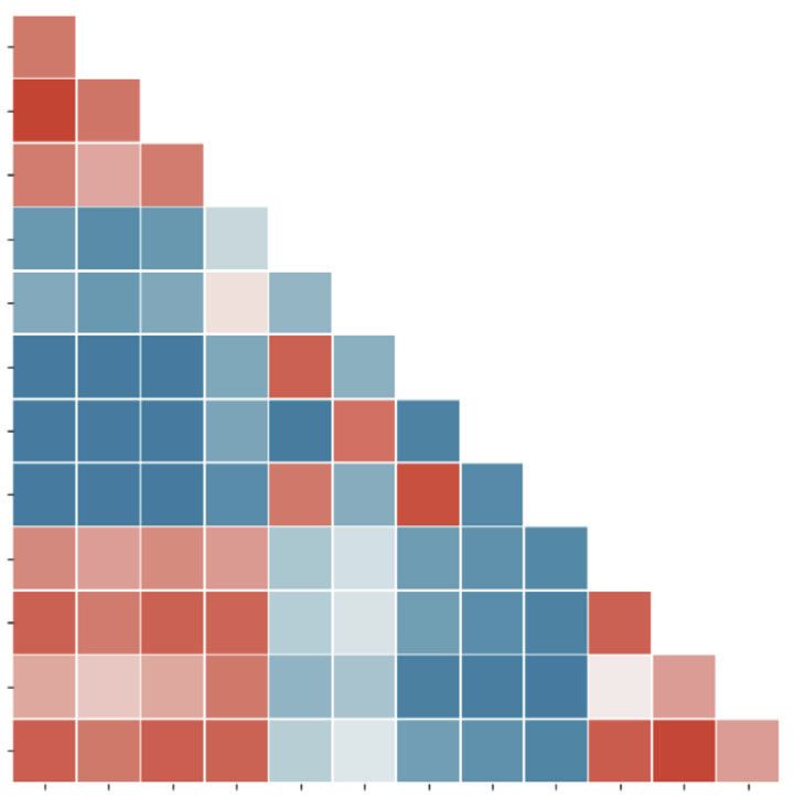
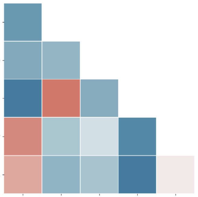
THALER et al. 11

 A B

F I G U R E 8 Results of the correlation study of the relevant candidates of the earthquake intensity measures: (a) possible input parameters
and (b) finally chosen input parameters

After exceeding the yield criterion of = 235 GPa, the stiffness is reduced to 10% of the initial stiffness 2 = 0.1 1 . The
 kg
density of the material is = 7850 3 . A rectangular hollow cross-section (0.3 m × 0.4 m), with a thickness of 0.03 m,
 m
is chosen for the beams. In order to model the mass of the slabs, point masses of 3000 kg are added to the nodes of each
beam. The columns are modeled as a hollow square cross-section with a width of 0.3 m and a thickness of 0.03 m.
 The structure is subjected to the generated earthquakes, while the structural response is calculated using the Newton–
Raphson algorithm.59 Analyzing the structural response reveals that maximum plastic stress–strain relations occur within
the cross-sections of the beam in the region of the frame corners. Based on this observation, we introduce the story drift
ratio as a measure of the level of damage. A peak story drift ratio equal to 4.5% corresponds to a full plastification in the
frame corner cross-section of the structure and is in line with the existing literature.69

4.2 Input parameters and hyperparameter search

In this section, the choice of the input parameters for the neural network estimation is briefly discussed. However, the
extent of the study carried out within this project does not necessarily ensure the highest neural network performance.
Investigations based on different parameters for the inputs using a classical neural network approach can be found in
the existing literature.60 Notably, Arias intensity, characteristic intensity, and CAV are chosen more often as intensity
measures as input for the neural network prediction.61, 62
 As mentioned in Section 3.4, earthquake intensity measures are used to characterize the generated accelerations. These
measures can be derived from the generated accelerations and from response spectra. In order to keep the neural network
small and fast, we want to use few input parameters, and therefore, only the most relevant features. This input parameter
search is started by using only one input measure. The input parameter that leads to the best performance of the neural
network is then the first fixed input quantity. Furthermore, the choice of the next input could be made by ranking the
performance of all the remaining input parameters. However, we want to ensure that the neural network is not fed by too
much redundant data. This is based on the assumption that highly correlated input features will not result in beneficial
output predictions. Thus, we also pay attention to the correlations between the input values, as shown in Figure 8.
 The spectral displacement at the natural period of the structure ( 1 ) is observed to be the best single input parameter.
This is not surprising because it has the highest correlation with the failure criterion chosen from the structural response.
Therefore, this intensity measure is chosen as the fixed input parameter. Due to the correlations shown in Figure 8 and
their performance in combination with the spectral displacement at the natural period ( 1 ), further parameters are
chosen. Stepwise increasing of the number of input parameters and taking into account previous studies,29, 60–62 the

12 THALER et al.

F I G U R E 9 Input parameter distributions visualized as violin plots;67 distributions of the intensity measures from the generated acceler-
ations without additional intensity variation (A) and with additional intensity variation (B)

following intensity measures are chosen: spectral acceleration at the natural period ( 1 ), velocity spectrum intensity
∫ , spectral displacement at the natural period ( 1 ), CAV, peak ground acceleration (PGA) and EPA.
 Additionally to the choice of the input parameters, the distribution of these chosen features is important for the sim-
ulation strategy proposed in Section 3.4. The violin plots,67 as shown in Figure 9, provide the information about these
 − 
distributions. The values haven been standardized, = , to compare all the input features. Hereby, denotes the
 2 
expected value and is the standard deviation. The standardization of these values uses the same mean and standard
deviation calculated from the distributions of the generated accelerations without additional variation. In Figure 9(A),
these distributions are shown, whereas Figure 9(B) shows the distributions of the intensity measures of the generated
accelerations with additional variation. This figure reveals that the intensity measures chosen behave as desired to reach
the objectives of this paper. They are stretched by the use of the additional factor in the white noise generation, as
described in Section 3.4. The input parameters are scattered over a larger range, and therefore, cover a larger prediction
range regarding possible inputs for the Monte Carlo simulation later.
 We applied the training strategy, as shown in Figure 6, using a training input of 400 randomly chosen samples of the
classical simulation sample set. A hyperparameter search is performed on this data set. The neural network architecture is
found by varying the hidden layer between one and four layers, with up to 30 units per layer. The parameters are modified
until a satisfying convergence is achieved. In order to avoid overfitting, a validation set of 100 further samples is used. Next
to the neural network architecture, the most common activation functions have been tested.44 This includes logistic sig-
 1 2 −1
moid ( ) = , hyperbolic tangent ( ) = 2 , and rectified linear units ( ) = max (0, ). We note that the neural
 1+ − +1
network, found by the hyperparameter tuning procedure, performs well in respect of the given task. The architecture of
the neural network consists of three hidden layers with 10 neurons in each layer. Rectified linear activation functions are
used for the neurons of the hidden layers, whereas the output unit has a linear activation function.

4.3 Results

For the numerical demonstration of the new strategy, a neural network is trained using 400 scattered samples with higher
intensity variance, as illustratively shown in Figure 5(C) and discussed in Section 3.4. The factor , introduced in Sec-
tion 3.4, is uniformly randomized between 0.8 and 1.5 and multiplied by the generated white noise. This obviously results
in a higher number of extreme events, as shown in Figure 9 and discussed in Section 4.2. The method is compared with the
full benchmark Monte Carlo solution, calculated by the finite element method and the neural network method following
the classical training procedure.
 To obtain a feasible benchmark result for the Monte Carlo simulation, the peak story drift ratios are evaluated for a
number of 104 earthquake samples. Using the in-house tool, the evaluation of the structural response takes between 80
and 160 seconds for one earthquake sample, dependent on the severity of plastic deformation. The mean simulation time

THALER et al. 13

TA B L E 2 Comparison of computational efforts between the crude Monte Carlo simulation and the new proposed Monte Carlo strategy
 Full evaluation Response spectra
 Simulation time Simulation time Total time
 Simulation strategy Samples (seconds) Samples (seconds) (seconds)
 Crude Monte Carlo 104 120 (–) (–) 1.2 × 106
 4
 Proposed new strategy 400 120 10 1 5.8 × 104

F I G U R E 1 0 Structural response to one sample excitation. Story drift ratio of the first, second, and third floors depicted in black, red, and
blue color, respectively

for 104 samples is 124 seconds. The calculation of the response spectra and the evaluation of the inputs for the neural
network, i.e., the chosen set of intensity measures, takes around 1 second.
 For the neural network prediction, the input features need to be extracted from the acceleration histories and the cor-
responding response spectra. Furthermore, the training targets need to be evaluated. Thus, the structural response is cal-
culated with the finite element method for the training samples, and the peak story drift ratios are extracted. Once both
neural networks perform well on the training and validation sets, they are used to predict the full response statistics of the
104 samples. Even though the response spectra must still be calculated for the input of the neural network, the speedup of
this simulation compared to the crude Monte Carlo is outstanding, as presented in Table 2. The time needed to predict the
response using neural networks is much smaller, and therefore, neglected in the comparison of the computational efforts.
For the numerical example in this paper, the whole neural network approach is 20 times faster, if 400 samples are used
for the initial training subset.
 Figure 11 shows the results of the crude Monte Carlo simulation, evaluated by the finite element method and the neural
network enhanced Monte Carlo strategies, and trained by taking samples from the expected feature range (classical proce-
dure) or by the proposed extended feature range (new strategy). Overall, the probability density function of the response
statistics (see Figure 11A) of the neural network enhanced Monte Carlo evaluation with classical training strategy is in

F I G U R E 1 1 Results of Monte Carlo simulation with 104 samples: (A) probability density function and (B) complementary cumulative
distribution function

14 THALER et al.

line with the standard Monte Carlo method. However, as expected, the complementary cumulative distribution func-
tion (Figure 11B) reveals that the tail region is badly predicted by the Monte Carlo strategy with the classically trained
neural network.
 Using more samples of unlikely earthquakes for the training of the neural network covers a wider range of inputs, which
leads to better predictions in the tail region, as shown in Figure 11(B). The probability density function in Figure 11(A)
shows that the neural network with classical training outperforms the neural network with extended training in the mean
region. Comparing the value of the peak story drift ratios that exceeded a certain value by the probability of = 50%, we
find that the standard neural network approach has a percentage error of only 0.3%, whereas the proposed method deviates
by 6.2% from the solution of the crude Monte Carlo simulation. However, in the tail region, the neural network with the
extended training strategy considerably outperforms the neural network with classical training.
 In this paper, we define structural failure if the peak story drift ratio exceeds a value of 4.5%, as shown by the vertical lines
in Figures 11(A) and 11(B). This assumption is based on the plastification of the structure, as discussed in Section 4.1, and
in line with the relevant literature.69 One can observe that the classical neural network training strategy fails to predict the
probability of failure. However, the extended strategy improves the quality of the estimation significantly. The prediction of
the probability of failure using the proposed strategy reveals a percentage error of 1.4%, whereas the classical approach fails
completely, and therefore, reveals an error of 100%. From another perspective, one can also be interested in the peak story
drift, which is exceeded with a probability of 0.1% or 1%. The peak story drift of the crude Monte Carlo simulation exceeds
the values of PSDR( = 1%) = 3.90% and PSDR( = 0.1%) = 4.67%, with a probability of 1% and 0.1%, respectively. The
standard neural network approach estimates the values PSDR( = 1%) = 3.44% and PSDR( = 0.1%) = 3.80%, whereas
the extended approach predicts the values PSDR( = 1%) = 3.87% and PSDR( = 0.1%) = 4.62%. This results in a per-
centage error of 11.8% for the classical method and 0.6% for the extended method, if the values with a probability of 1% are
compared. This is even more visible if the chosen limit is the probability of 0.1%. The errors are found to be 18.6% for the
classical training and 0.9% for the extended training.
 We conclude that a feedforward neural network with three hidden layers and 10 neurons in each layer is able to predict
the peak story drift ratios for the problem in this paper. Furthermore, the training of the neural network is efficient, since
it contains a rather small number of parameters. Therefore, the number of time-consuming finite element calculations
for the training set can be kept small.

5 CONCLUSION

In this paper, we developed a neural network enhanced Monte Carlo simulation that provides the response statistics of
a ground accelerated structure. The new strategy reveals an outstanding efficiency when compared to the crude Monte
Carlo method and ensures a reliable prediction in the tail end of the distribution.
 The main benefit of using neural networks to predict the response statistics is computational savings. However, in order
to train a neural network, a certain number of calculated samples are necessary. To ensure that a neural network is able to
perform well on a given task, it is crucial to provide the necessary information. The proposed method enables the neural
network to predict low probability events in the tail region of the distribution with higher accuracy compared to a stan-
dard neural network approach. The computational effort to calculate the full response sample set decreases significantly
compared to the standard Monte Carlo procedure.
 We intentionally use a small feedforward neural network, which requires a rather smaller number of training samples,
and therefore, a short training time period is sufficient to obtain accurate response statistics. Six input parameters, chosen
from possible earthquake intensity measures, are sufficient to provide accurate response statistics.
 By contrast with conventional machine learning approaches, we propose an adaptation to problems in earthquake
engineering and used an extended sample range for the neural network training, taking site-dependent behavior into
account. In that respect, we concentrate on accurately predicting the response statistics near structural failure and ensure
that the neural network is sufficiently trained in this particular region. The major advantage of this approach is that the
neural network does not have to extrapolate the predictions in case of very rare events, which would lead to unacceptably
inaccurate predictions in the tail end of the distribution. A side effect of the proposed method is the accuracy loss in
high probability events. The conventional approach, using the standard sample range, is able to predict this region better.
However, to evaluate the probability of structural failure, this trade-off can be neglected. This idea makes our method
particularly effective for the prediction of events near structural failure.

THALER et al. 15

ORCID
Denny Thaler https://orcid.org/0000-0002-1153-3203
Marcus Stoffel https://orcid.org/0000-0001-8756-2310
Bernd Markert https://orcid.org/0000-0001-7893-6229
Franz Bamer https://orcid.org/0000-0002-8587-6591

REFERENCES
 1. Der Kiureghian A. Structural reliability methods for seismic safety assessment: a review. Eng Struct. 1996;18(6):412-424.
 2. Kafali C, Grigoriu M. Seismic fragility analysis: application to simple linear and nonlinear systems. Earthq Eng Struct Dyn. 2007;36(13):1885-
 1900.
 3. Fajfar P, Dolšek M. A practice-oriented estimation of the failure probability of building structures. Earthq Eng Struct Dyn. 2012;41(3):531-
 547.
 4. Pinto P. Reliability methods in earthquake engineering. Progr Struct Eng Mater. 2001;3(1):76-85.
 5. Ghobarah A. Performance-based design in earthquake engineering: state of development. Eng Struct. 2001;23(8):878-884.
 6. Bucher, C. Computational Analysis of Randomness in Structural Mechanics. London: Tayler & Francis; 2009.
 7. Shinozuka M. Monte Carlo solution of structural dynamics. Comput Struct. 1972;2(5):855-874.
 8. Hurtado J, Barbat H. Monte Carlo techniques in computational stochastic mechanics. Arch Comput Methods Eng. 1998;5:3-30.
 9. Ellingwood B. Earthquake risk assessment of building structures. Reliab Eng Syst Saf. 2001;74:251-262.
10. Elnashai, A, Di Sarno, L. Fundamentals of Earthquake Engineering. Chichester, UK: Wiley; 2008.
 11. Bamer F, Amiri A, Bucher C. A new model order reduction strategy adapted to nonlinear problems in earthquake engineering. Earthq
 Eng Struct Dyn. 2017;46(4):537-559.
12. Bamer F, Markert B. An efficient response identification strategy for nonlinear structures subject to nonstationary generated seismic
 excitations. Mech Based Des Struct Machine. 2017;45:313-330.
13. Bamer F, Bucher C. Application of the proper orthogonal decomposition for linear and nonlinear structures under transient excitations.
 Acta Mech. 2012;223:2549-2563.
14. Bucher C. Asymptotic sampling for high-dimensional reliability analysis. Probabilistic Eng Mech. 2009;24(4):504-510.
15. Breitung K. Asymptotic approximations for multinormal integrals. J Eng Mech. 1984;110(3):357-366.
16. Caughey TK,. Equivalent linearization techniques. J Acoust Soc Am. 1963;35(11):1706-1711.
17. Atalik TS, Utku S. Stochastic linearization of multi-degree-of-freedom non-linear systems. Earthq Eng Struct Dyn. 1976;4(4):411-420.
18. Casciati F, Faravelli L, Hasofer A. A new philosophy for stochastic equivalent linearization. Probabilistic Eng Mech. 1993;8(3):179-185.
19. Yi S, Wang Z, Song J. Bivariate Gaussian mixture–based equivalent linearization method for stochastic seismic analysis of nonlinear struc-
 tures. Earthq Eng Struct Dyn. 2018;47(3):678-696.
20. Fujimura K, Der Kiureghian A. Tail-equivalent linearization method for nonlinear random vibration. Probabilistic Eng Mech. 2007;22(1):63-
 76.
21. Alanis, AY, Arana-Daniel, N, López-Franco, C. Artificial Neural Networks for Engineering Applications. St. Louis, Missouri, Academic Press:
 Elsevier; 2019.
22. Stoffel M, Bamer F, Markert B. Artificial neural networks and intelligent finite elements in non-linear structural mechanics. Thin-Walled
 Struct. 2018;131:102-106.
23. Stoffel M, Bamer F, Markert B. Neural network based constitutive modeling of nonlinear viscoplastic structural response. Mech Res Com-
 mun. 2019;95:85-88.
24. Stoffel M, Gulakala R, Bamer F, Markert B. Artificial neural networks in structural dynamics: a new modular radial basis function approach
 vs. convolutional and feedforward topologies. Comput Methods Appl Mech Eng. 2020;364:112989.
25. Stoffel M, Bamer F, Markert B. Deep convolutional neural networks in structural dynamics under consideration of viscoplastic material
 behaviour. Mech Res Commun. 2020;108:103565.
26. Koeppe A, Bamer F, Markert B. An intelligent nonlinear meta element for elastoplastic continua: deep learning using a new time-
 distributed residual U-net architecture. Comput Methods Appl Mech Eng. 2020;366:113088.
27. Koeppe A, Bamer F, Markert B. An efficient Monte Carlo strategy for elasto-plastic structures based on recurrent neural networks. Acta
 Mech. 2019;230:3279-3293.
28. Heider Y, Wang K, Sun WC,. SO(3)-invariance of informed-graph-based deep neural network for anisotropic elastoplastic materials. Com-
 put Methods Appl Mech Eng. 2020;363:112875.
29. Sun H, Burton HV, Huang H. Machine learning applications for building structural design and performance assessment: state-of-the-art
 review. J Build Eng. 2021;33:101816.
30. Molas G, Yamazaki F. Neural networks for quick earthquake damage estimation. Earthq Eng Struct Dyn. 1995;24(4):505-516.
31. Huang CS, Hung SL, Wen CM, Tu TT,. A neural network approach for structural identification and diagnosis of a building from seismic
 response data. Earthq Eng Struct Dyn. 2003;32(2):187-206.
32. Mangalathu S, Sun H, Nweke CC, Yi Z, Burton HV,. Classifying earthquake damage to buildings using machine learning. Earthq Spectra.
 2020;36(1):183-208.

16 THALER et al.

33. Hurtado JE, Alvarez DA,. Neural-network-based reliability analysis: a comparative study. Comput Methods Appl Mech Eng. 2001;191(1):113-
 132.
34. Chojaczyk A, Teixeira A, Neves L, Cardoso J, Guedes Soares C. Review and application of Artificial Neural Networks models in reliability
 analysis of steel structures. Struct Saf. 2015;52:78-89.
35. Thaler D, Bamer F, Markert B. A machine learning enhanced structural response prediction strategy due to seismic excitation. Proc Appl
 Math Mech. 2020;20:e202000294.
36. Vazirizade S, Nozhati S, Zadeh M. Seismic reliability assessment of structures using artificial neural network. J Build Eng. 2017;11:230-235.
37. Kiani J, Camp C, Pezeshk S. On the application of machine learning techniques to derive seismic fragility curves. Comput Struct.
 2019;218:108-122.
38. Gomes H, Awruch A. Comparison of response surface and neural network with other methods for structural reliability analysis. Struct
 Saf. 2004;26(1):49-67.
39. Burton HV,. Estimating aftershock collapse vulnerability using mainshock intensity, structural response and physical damage indicators.
 Struct Saf. 2017;68:85-96.
40. Zhang Y, Burton HV, Sun H, Shokrabadi M. A machine learning framework for assessing post-earthquake structural safety. Struct Saf.
 2018;72:1-16.
41. Zhang Y, Burton HV,. Pattern recognition approach to assess the residual structural capacity of damaged tall buildings. Struct Saf.
 2019;78:12-22.
42. Mignan A, Broccardo M. Neural network applications in earthquake prediction (1994–2019): meta-analytic and statistical insights on their
 limitations. Seismol Res Lett. 2020;91(4):2330-2342.
43. Hornik K. Approximation capabilities of muitilayer feedforward networks. Neural Netw. 1991;4(7):251-257.
44. Goodfellow, I, Bengio, Y, Courville, A. Deep Learning. Cambridge, MA; London: MIT Press; 2016. http://www.deeplearningbook.org.
45. Rumelhart DE, Hinton GE, Williams RJ,. Learning representations by back-propagating errors. Nature. 1986;323:533-536.
46. Kingma, D, Ba, J. Adam: a method for stochastic optimization. In: International Conference on Learning Representations. 2015.
47. Kruse, R, Borgelt, C, Braune, C, Klawonn, F, Moewes, C, Steinbrecher, M. Computational Intelligence, Eine methodische Einführung in
 Künstliche Neuronale Netze, Evolutionäre Algorithmen, Fuzzy-Systeme und Bayes-Netze. Wiesbaden: Springer Vieweg; 2015. ISBN 978-3-
 658-10904-2.
48. Rossum, G. Python Reference Manual. Technical Report CWI (Centre for Mathematics and Computer Science), NLD; 1995.
49. Abadi, Mea. TensorFlow: Large-Scale Machine Learning on Heterogeneous Systems. https://www.tensorflow.org 2015.
50. Kanai, K. Semi-Empirical Formula for the Seismic Characteristics of the Ground, Vol. 35. Tokyo: Bulletin of the Earthquake Research Insti-
 tute, University of Tokyo; 1957:309-325.
51. Tajimi, H. A statistical method of determining the maximum response of a building structure during an earthquake. In: Proceedings of the
 2nd World Conference on Earthquake Engineering, Tokio. 1960:781-798.
52. Fan F, Ahmadi G. Nonstationary Kanai-Tajimi models for El Centro 1940 and Mexico City 1985 earthquakes. Probabilistic Eng Mech.
 1990;5(4):171-181.
53. Rofooei F, Mobarake A, Ahmadi G. Generation of artificial earthquake records with a nonstationary Kanai-Tajimi model. Eng Struct.
 2001;23:827-837.
54. Kallianpur, G, Karandikar, R. White Noise Theory of Prediction, Filtering and Smoothing. Boca Raton, FL: Taylor & Francis; 1988.
55. Bamer F, Markert B. A nonlinear visco-elastoplastic model for structural pounding. Earthq Eng Struct Dyn. 2018;47(12):2490-2495.
56. Bamer F, Strubel N, Shi J, Markert B. A visco-elastoplastic pounding damage formulation. Eng Struct. 2019;197:109373.
57. Center for Engineering Strong Motion Data. Kobe Takarzuka Earthquake Measurement 1995-01-16 20:46:52 UTC. Virtual Data Center 2016.
 www.strongmotioncenter.org/.
58. Bathe, KJ. Finite Element Procedures. Englewood Cliffs, NJ: Prentice Hall; 1996.
59. Chopra, A. Dynamics of Structures, Theory and Applications to Earthquake Engineering. Englewood Cliffs, NJ: Prentice Hall; 2007.
60. Morfidis K, Kostinakis K. Seismic parameters’ combinations for the optimum prediction of the damage state of R/C buildings using neural
 networks. Adv Eng Softw. 2017;106:1-16.
61. Jough FKG, Şensoy S. Prediction of seismic collapse risk of steel moment frame mid-rise structures by meta-heuristic algorithms. Earthq
 Eng Eng Vib. 2016;15(4):743-757.
62. Mitropoulou CC, Papadrakakis M. Developing fragility curves based on neural network IDA predictions. Eng Struct. 2011;33(12):3409-3421.
63. Bianchini, M, Diotallevi, P, Baker, JW. Prediction of inelastic structural response using an average of spectral accelerations. In: Proceedings
 of the 10th International Conference on Structural Safety and Reliability (ICOSSAR 09). 2009.
64. Eads L, Miranda E, Lignos DG,. Average spectral acceleration as an intensity measure for collapse risk assessment. Earthq Eng Struct Dyn.
 2015;44(12):2057-2073.
65. Kazantzi A, Vamvatsikos D. Intensity measure selection for vulnerability studies of building classes. Earthq Eng Struct Dyn. 2015;44:2677-
 2694.
66. Adam, C, Kampenhuber, D, Ibarra, LF. Optimal intensity measure based on spectral acceleration for P-delta vulnerable deteriorating
 frame structures in the collapse limit state. Bull Earthq Eng. 2017;15(10);4349-4373.
67. Hintze JL, Nelson RD,. Violin plots: a box plot-density trace synergism. Am Stat. 1998;52(2):181-184.
68. Liang X, Mosalam KM,. Lyapunov stability and accuracy of direct integration algorithms applied to nonlinear dynamic problems. J Eng
 Mech. 2016;142:04016022.

THALER et al. 17

69. FEMA 356. Prestandard and Commentary for the Seismic Rehabilitation of Buildings. Washington, DC: Federal Emergency Management
 Agency; 2000.

 How to cite this article: Thaler D, Stoffel M, Markert B, Bamer F. Machine-learning-enhanced tail end
 prediction of structural response statistics in earthquake engineering. Earthquake Engng Struct Dyn. 2021;1–17.
 https://doi.org/10.1002/eqe.3432