A general framework for a joint calibration of VIX and VXX options
←
→
Page content transcription
If your browser does not render page correctly, please read the page content below
A general framework
                                                      for a joint calibration of VIX and VXX options
                                                     Martino Grasselli1,2 , Andrea Mazzoran1 , and Andrea Pallavicini3,4
                                            1
                                              Department of Mathematics, University of Padova, Via Trieste 63 Padova 35121, Italy. Email:
                                                                               andreamazzoran@hotmail.it
                                            2
                                              Devinci Research Center, Léonard de Vinci Pôle Universitaire, 92 916 Paris La Défense, France.
                                                                              Email: grassell@math.unipd.it
arXiv:2012.08353v1 [q-fin.MF] 15 Dec 2020

                                               3
                                                 Department of Mathematics, Imperial College, London SW7 2AZ, United Kingdom. Email:
                                                                               a.pallavicini@imperial.ac.uk
                                                        4
                                                          Financial Engineering, Banca IMI, largo Mattioli 3 Milano 20121, Italy.

                                                                                 December 16, 2020

                                                                                       Abstract
                                                    We analyze the VIX futures market with a focus on the exchange-traded notes
                                                 written on such contracts, in particular, we investigate the VXX notes tracking the
                                                 short-end part of the futures term structure. Inspired by recent developments in
                                                 commodity smile modeling, we present a multi-factor stochastic local-volatility model
                                                 able to jointly calibrate plain vanilla options both on VIX futures and VXX notes.
                                                 We discuss numerical results on real market data by highlighting the impact of model
                                                 parameters on implied volatilities.

                                            JEL classification codes: C63, G13.
                                            AMS classification codes: 65C05, 91G20, 91G60.
                                            Keywords: Local volatility, Stochastic volatility, VIX, VIX futures, VXX.

                                                                                           1
Contents
1 Introduction 3
2 Stochastic local-volatility models 6
3 Smile modelling for ETP on futures strategies 7
3.1 ETP on futures strategies . . . . . . . . . . . . . . . . . . . . . . . . . . . . 7
3.2 Modeling the ETP smile . . . . . . . . . . . . . . . . . . . . . . . . . . . . . 8
4 The VXX ETN strategy 11
4.1 Definition of the ETN strategy . . . . . . . . . . . . . . . . . . . . . . . . . 12
4.2 The local correlation . . . . . . . . . . . . . . . . . . . . . . . . . . . . . . . 12
4.3 Model specification . . . . . . . . . . . . . . . . . . . . . . . . . . . . . . . . 14
5 Numerical illustration on a real data set 15
5.1 VIX and VXX data sets . . . . . . . . . . . . . . . . . . . . . . . . . . . . . 15
5.2 Parameter sensitivities . . . . . . . . . . . . . . . . . . . . . . . . . . . . . . 16
5.3 Joint fit of VIX and VXX market smiles . . . . . . . . . . . . . . . . . . . . 19
6 Conclusion and further developments 23
21 Introduction
In recent years, it has become increasingly common to consider volatility as its own asset
class. The great financial crisis accelerated the demand for volatility instruments and
many different volatility products have been invented and are now available to trade,
see Sussman and Morgan (2012). Created by the CBOE1 in 1993, the VIX index is by
far one of the most popular volatility instruments and it is considered as a landmark by
most market players. It is calculated and disseminated on a real-time basis by the CBOE
and represents the market’s expectation of 30-day forward-looking volatility. Derived
from the price inputs of the S&P 500 index options, it provides a measure of market risk
and investors’ sentiments. Investors, research analysts and portfolio managers look at
VIX values as a way to measure market risk, fear and stress before they take investment
decisions, this being a reason why it is also known as the “Fear Index". Indeed, when the
VIX is rising, active investors will typically try to hedge their positions by taking short
position on the market, while when the VIX is falling, active investors will closely watch
the market to increase their long positions. During its origin, the formula that determined
the VIX was tailored to S&P 100 index option prices, more precisely it was calculated as
a weighted measure of the 30-day implied volatility of eight S&P 100 at-the-money put
and call options, when the derivatives market had limited activity and was in growing
stages. Ten years later, its calculation has been slightly revised when people started using
a wider set of options based on the broader S&P 500 index, an expansion which allows
for a more accurate view of investors’ expectations on future market volatility. But apart
from its role as a risk indicator, nowadays it is possible to directly invest in volatility as
an asset class by means of VIX derivatives. Specifically, VIX became tradable via futures
in 2004 and via options in 2006, hence providing market participants with the ability to
trade liquid volatility products based on the VIX, see Whaley (2009). Since then, volumes
on VIX futures and options drastically increased. For example, in 2015, the VIX became
the second most traded underlying in the CBOE options market2 , right after the S&P 500
itself.
As derivatives on the VIX may be inaccessible to non-institutional players, mainly
due to the large notional sizes of the contracts as currently designed by the CBOE, some
exchange-traded notes (ETN) on the VIX were introduced. In 2009, Barclays launched
the first two ETN’s on the VIX: VXX3 and VXZ. The VXX ETN was the first exchange-
traded product (ETP) on VIX futures, issued shortly after the inception of the VIX futures
indices. The VXX is a non-securitized debt obligation, similar to a zero-coupon bond, but
with a redemption value that depends on the level of the S&P 500 (SPX) VIX Short-
Term Futures Total Return index (SPVXSTR). The SPVXSTR tracks the performance
of a position in the nearest and second-nearest maturing VIX futures contracts, which
is rebalanced daily to create a nearly constant 1-month maturity. In other words, VXX
mimics the behaviour of the VIX, namely of the 30-day forward-looking volatility, using a
replicable strategy based on futures on VIX. Since 2009 then, ETN’s on the VIX flourished:
there currently exist more than thirty of them, with several billion dollars in market caps
and daily volumes (see Alexander and Korovilas (2013) for a comprehensive empirical
1
See the white paper of CBOE in 2014 titled CBOE Volatility Index, available at https://www.cboe.
com/micro/vix/vixwhite.pdf.
2
See the white paper of CBOE in 2016 titled CBOE holdings reports trading volume for 2015,
available at http://ir.cboe.com/~/media/Files/C/CBOE-IR-V2/press-release/2016/cboe-holdings-
volume-report-december-2015.pdf.
3
See the VXX Prospectus of Barclays available at https://www.ipathetn.com/US/16/en/instruments.
app?searchType=text&dataType=html&searchTerm=VXX
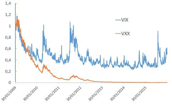
3Figure 1: Prices in dollars of VIX (in blue) and VXX (in red), normalized to 1 on 30
January 2009.
study on VIX ETN’s).
One of the main reasons for the high interest in these products is that VIX derivative
positions can be used to provide protection against the risks inherent in the S&P500 index,
especially in downturns. At the same time, VIX derivatives allow investors to achieve
exposure to S&P500 volatility more cheaply than by using traditional derivatives on this
broad stock market index. However, the poor performance of some of these derivative
assets during decreasing volatility periods has raised some concerns about their risks among
market players and regulators4 . Even though VXX is very heavily traded, it has lost
99.84% of its value since inception and Figure 1 shows the remarkable underperformance
of VXX compared to VIX. Whereas many market players use VXX as a proxy for trading
VIX in a cheap manner, in the VXX Prospectus3 Barclays warns VXX holders that “Your
ETN is not Linked to the VIX index and the value of your ETN may be less than it would
have been had your ETN been linked to the VIX Index".
In literature, attempts to model VIX can be divided in two strands: on the one hand,
the consistent-pricing approach models the joint (risk-neutral) dynamics of the S&P 500
and the VIX with, most often, the aim of pricing derivatives on the two indices in a consis-
tent manner, on the other hand, the stand-alone approach directly models the dynamics
of the VIX.
In the former case, we can include the work of Cont and Kokholm (2013) and references
therein, while more applications can be found in the work of Gehricke and Zhang (2018),
where they propose a consistent framework for S&P 500 (modelled with a Heston-like
specification) and the VIX derived from the square root of the variance swap contract.
On top of that, they construct the VXX contract from the Prospectus and show that
the roll yield of VIX futures drives the difference between the VXX and VIX returns
on time series. More recently, in the paper of Gatheral et al. (2020), a joint calibration
of SPX and VIX smile has been successfully obtained using the quadratic rough Heston
4
See the white paper of Bloomberg in 2012 titled SEC said to review Credit Suisse VIX Note
available at https://www.bloomberg.com/news/articles/2012-03-29/sec-said-to-review-credit-
suisse-vix-note.
4model, while Guyon (2020b) builds up a non-parametric discrete-time model that jointly
and exactly calibrates to the prices of SPX options, VIX futures and VIX options. We
also mention the work of Guyon (2020a), where the author investigates conditions for the
existence of a continuous model on the S&P 500 index (SPX) that calibrates the full surface
of SPX and VIX implied volatilities, and the paper of De Marco and Henry-Labordere
(2015), where the authors bound VIX options from vanilla options and VIX futures, which
leads to a new martingale optimal transport problem that they solve numerically.
In the latter case, the first stand-alone model for the VIX was proposed by Whaley,
see Whaley (1993), where he models the spot VIX as a geometric Brownian motion, hence
enabling to price options on the VIX in the Black and Scholes framework, but failing to
capture the smile effect and the mean-reversion of volatility processes, which is necessary
in order to fit the term structure of futures prices (Schwert (1990), Pagan and Schwert
(1990) and Schwert (2011)). We cite also the attempt of Drimus and Farkas (2013) based
on local volatility. Since then, numerous stand-alone models have been proposed for the
VIX. We refer to Bao et al. (2012) and Lin (2013) for a detailed review on that strand of
literature.
The literature on VXX is limited. To our knowledge, there are only a few theoretical
studies which propose a unified framework for VIX and VXX. Existing studies on the
VXX (Bao et al. (2012)) typically model the VXX in a stand-alone manner, which does
not take into account the link between VIX and VXX. As a consequence, the loss for
VXX when the VIX is in contango cannot be anticipated in such models. In the recent
paper of Gehricke and Zhang (2020), they analyze the daily implied volatility curves of the
VXX options market alone (where they consider the implied volatility as a function of the
moneyness through quadratic polynomial regressions), providing a necessary benchmark
for developing a VXX option pricing model.
We also mention the work of Grasselli and Wagalath (2020), where the authors were
able to link the properties of VXX to those of the VIX in a tractable way. In particular,
they quantify the systematic loss observed empirically for VXX when the VIX futures
term-structure is in contango and they derive option prices, implied volatilities and skews
of VXX from those of VIX in infinitesimal developments. The affine stochastic volatility
model of Grasselli and Wagalath (2020) exploits the FFT methodology in order to price
futures and options on VIX, while a Monte Carlo simulation is performed in order to
compare the resulting smile on the VXX implied by the calibrated model with the one
provided by real market data. The results are not completely satisfactory, which is not
surprising, since the VXX can be seen as an exotic path-dependent product on VIX, so
that the information regarding the smile on vanillas (on VIX) are well known to be not
enough to recover the whole information concerning path dependent products (see for
instance Bergomi (2015)).
In the present paper we leave the pure stochastic volatility model for the VIX and
we introduce a stochastic local-volatility model (SLV), that is able to jointly calibrate
VIX and VXX options in a consistent manner. The same methodology can be easily
extended to other pairs of futures contracts and notes. SLV models are the de-facto
industry standard in option pricing since they allow to join the advantages of stochastic
volatility models with a good fit of plain options. They were first introduced in Lipton
(2002), while a first efficient PDE-based calibration procedure was presented in Ren et al.
(2007). In the present paper, since we investigate multi-factor models, we follow the
calibration approach of Guyon and Henry-Labordère (2012), which is based on a Monte
Carlo simulation. The SLV model we introduce for the VIX futures starts from the work
of Nastasi et al. (2020), where the problem of modelling futures smiles for commodity
5assets in a flexible but parsimonious way is discussed. In particular, here we investigate a
multi-factor extension of such model which is tailored to describe VIX futures prices, and
to allow a joint calibration of VIX and VXX plain vanilla options.
The key feature of our model is the possibility to decouple the problems of calibrating
VIX plain vanilla options, which are recovered by a suitable choice of the local-volatility
function, from the more complex task of calibrating the plain vanilla options on the VXX
notes. We recall that in our approach the VXX notes are exotic path-dependent product
written on VIX futures. We solve the second problem by introducing a local-correlation
function between the factors driving the futures prices, and by properly selecting the
remaining free dynamics parameters. The calibration of the local correlation function is
inspired by the work of Guyon (2017).
The paper is organized as follows. In Section 2 we give a brief overview of SLV models,
highlighting their properties and the main advantages in using these models. In Section 3,
we present the general setting of our model. We start from the evolution of a general ETP
and their underlying futures contracts, then we describe how to calibrate futures prices
and options on futures. In Section 4 we adapt the general framework of the previous
section to the case of the VXX ETN strategy. In Section 5 a calibration exercise based on
real data along with numerical results and comparisons are presented, involving a joint fit
and a parameters sensitivity analysis. In Section 6 we draw some conclusion and remarks.
Needless to say, the views expressed in this paper are those of the authors and do not
necessarily represent the views of their institutions.
2 Stochastic local-volatility models
One of the main advantages of using local-volatility models (LV) is their natural modelling
of plain-vanilla market volatilities. Indeed, a LV model can be calibrated with extreme
precision to any given set of arbitrage-free European vanilla option prices. LV model
were first introduced by Dupire et al. (1994) and Derman and Kani (1994). Although
well-accepted, LV models have certain limitations, for example, they generate flattening
implied forward volatilities, see Rebonato (1999), that may lead to a mispricing of financial
products like forward-starting options.
On the other hand, stochastic volatility (SV) models, like the well known Heston
model, see Heston (1993), are considered to be more accurate choices for pricing forward
volatility sensitive derivatives, see Gatheral (2011). Although the SV models have desired
features for pricing, they often cannot be very well calibrated to a given set of arbitrage-
free European vanilla option prices. In particular, the accuracy of the Heston model for
pricing short-maturity options in the equity market is typically unsatisfactory.
One possible improvement to the previous issues is considering stochastic local-volatility
models (SLV), that take advantages of both LV and SV models properties. SLV models,
going back to Lipton (2002), are still an intricate task, both from a theoretical as well as a
practical point of view. The main advantage of using SLV models is that one can achieve
both a good fit to market series data and in principle a perfect calibration to the implied
volatility smiles. In such models the discounted price process (St )t≥0 of an asset follows
the stochastic differential equation (SDE)
dSt = St `(t, St )vt dWt , (2.1)
where (vt )t≥0 is some stochastic process taking real values, and `(t, K) is a sufficiently
regular deterministic function, the so-called leverage function, depending on time and on
6the current value of the underlying asset. Wt , as usual, is a one-dimensional Brownian
motion, possibly correlated with the noise driving the process v. Obviously, SV and
LV models are recovered by setting `(t, K) ≡ 1 or v ≡ 1, respectively. At this stage, the
stochastic volatility process (vt )t≥0 can be very general and by a slight abuse of terminology
we call (vt )t≥0 stochastic volatility as in the SV model.
The leverage function `(t, K) is the crucial part in this model. It allows in principle
to perfectly calibrate the market implied volatility surface. In order to achieve this goal,
` needs to satisfy the following relation:
2 (t, K)
σDup
` (t, K) = 2
2
, (2.2)
E vt St = K
where σDup denotes Dupire local-volatility function, see Dupire (1996). The familiar reader
would recognize in Equation (2.2) an application of the Markovian projection procedure,
a concept originating from the celebrated Gyöngy Lemma, see Gyöngy (1986), whose idea
basically lies in finding a diffusion which “mimics” the fixed-time marginal distributions
of an Itô process.
For the derivation of Equation (2.2), we refer to Guyon and Henry-Labordere (2013).
Notice that Equation (2.2) is an implicit equation for ` as it is needed for the computation
of E vt | St = K . It is a standard thing in SLV models and this in turn means that the
2
SDE for the price process (St )t≥0 is actually a McKean-Vlasov SDE, since the probability
distribution of St enters the characteristics of the equation. Existence and uniqueness
results for this equation are not obvious in principle, as the coefficients do not typically
satisfy standard conditions like for instance Lipschitz continuity with respect to the so-
called Wasserstein metric. In fact, deriving the set of stochastic volatility parameters for
which SLV models exist uniquely, for a given market implied volatility surface, is a very
challenging and still open problem. In the sequel, we will limit to investigate numerically
the validity of the assumption just stated in our specific framework.
3 Smile modelling for ETP on futures strategies
We start this section with a wider look to study the volatility smile of a generic ETP
based on futures strategies. Then, the results shown in this section will be applied to our
specific VXX case in Section 4.
3.1 ETP on futures strategies
We analyze an ETP based on a strategy of N futures contracts Ft (T ). If we assume that
the ETP strategy itself is not collateralized and it requires a proportional fee payment φt ,
we can write the strategy price process Vt as given by
N
dVt dFt (Ti )
= (rt − φt )dt + (3.3)
X
ωti ,
Vt i=1
Ft (Ti )
where rt is the risk-free rate. Moreover, we assume that the futures contracts and the
ETP are expressed in the same currency as the bank account based on rt . The processes
ωti represent the investment percentage (or weights) in the futures contracts, and they
are defined by the ETP term-sheet. Notice that the weights may depend on the whole
vector of futures prices. It is straightforward to extend the analysis to more general ETP
strategies based on total-return or dividend-paying indices. Moreover, we can introduce
securities in foreign currencies as in Moreni and Pallavicini (2017).
7We can consider as a first example the family of S&P GSCI commodity indices.
Exchange-Traded Commodity (ETC’s) tracking these indices are liquid in the market,
and they represent an investment in a specific commodity or commodity class. The in-
vestment is in the first nearby one-month future, but for the last five days of the contract,
where a roll over procedure is implemented to sell the first nearby and to buy the second
one. A second example are the volatility-based ETN’s VXX and VXZ. They represent
respectively an investment in short-term or in the long-term structure of VIX futures.
The investment is in a portfolio of futures mimicking a rolling one-month contract. In
Section 4 we will focus on the VXX case.
3.2 Modeling the ETP smile
We wish to jointly model the volatility smile of an ETP and of its underlying futures
contracts. Indeed, market quotes for ETP plain-vanilla options can be found on the
market. The main problem to solve is the fact that the price process of the ETP strategy
is non-Markov, since it depends on the futures contract prices, namely the vector process
[Vt , Ft (T1 ), . . . , Ft (TN )] is Markov.
We first start by modelling the marginal distribution of futures prices, then we proceed
to describe the full model. The marginal distribution is modelled by following the pro-
cedure developed in Nastasi et al. (2020) and originally implemented for the commodity
market. We consider that the futures prices Fts (Ti ) can be modelled in term of a common
process st , which we can identify with the price of a rolling futures contract. Futures
prices are defined in term of st as given by
R Ti
− a(u)du
Fts (Ti ) = F0 (Ti ) 1 − (1 − st ) e t (3.4)
where F0 (Ti ) are the futures prices as observed today in the market, and a is a non-
negative function of time. The value of the futures at maturity times t, which are not
quoted in the market, can be obtained by interpolation, but they are never used in actual
calculations. The driving risk process st is modelled by a mean-reverting local-volatility
dynamics, namely
dst = a(t) (1 − st ) dt + η (t, st ) st dWts , s0 = 1, (3.5)
where η is a positive and bounded function of time and price, to be determined by the
calibration of options of futures, and Wts is a standard Brownian motion under the risk-
neutral measure. As a consequence, the futures prices follows a local-volatility dynamics
given by
dFts (Ti ) = ηF (t, Ti , Fts (Ti )) dWts , (3.6)
where we define
R Ti
ηF (t, Ti , K) : = K − F0 (Ti ) 1 − e− t
a(u)du
η (t, kF (t, Ti , K)) , (3.7)
K
R Ti
kF (t, Ti , K) : = 1 − 1 − e t a(u)du . (3.8)
F0 (Ti )
Thus, plain-vanilla options on futures can be calculated as plain-vanilla options on the
process st , which, in turn, can be easily computed by means of the Dupire equation. More
precisely, given the dynamics in Equation (3.5), we have that the normalized call price
h i
c(t, k) := E (st − k)+ (3.9)
8satisfies the parabolic PDE
1
∂t c(t, k) = −a(t) − a(t)(1 − k)∂k + k 2 η 2 (t, k)∂k2 c(t, k), (3.10)
2
with boundary conditions
c(t, 0) = 1, c(t, ∞) = 0, c(0, k) = (1 − k)+ . (3.11)
A more detailed analysis and a proof of this (extended) Dupire equation can be found
in Nastasi et al. (2020, Proposition 4.1). Given the prices of options on futures from the
market, we can plug their corresponding normalized call prices in Equation (3.10), and
then solve it for the function η. Then, we can compute the futures local-volatility function
ηF (t, Ti , K), thanks to the mapping in Equation (3.7), and eventually recover the prices
of options on futures.
There is a vast literature on how to solve Equation (3.10) with the boundary con-
ditions (3.11), here we use an implicit PDE discretization method, as usually done for
solving the Dupire equation, see for example Gatheral (2011). We allow a mean-reversion
a(t) possibly different from zero when we are calibrating the model to options on futures.
On the other hand, options on the ETP spot price can be directly calibrated by a standard
local-volatility model, that is without a mean-reversion term. Hence, once a(t) is chosen,
we can calibrate to the market ηF (t, Ti , K) and ηV (t, K), as previously described.
Thanks to the normalized spot dynamics (3.5), we can price all futures options by
evaluating the PDE (3.10), and ETP options as well. In this way we implicitly obtain the
marginal probability densities of futures prices and ETP prices.
We are now looking for the joint probability densities of futures prices, in order to be
able to jointly model the dynamics of both the ETP strategy and its underlying futures. In
order to do that, we need to specify a non trivial correlation structure among the futures.
Notice that, for example, a one factor model based on the normalised spot dynamics, as in
Equation (3.5), would not be able to produce a non-trivial final correlation among futures,
see Nastasi et al. (2020, Section 5.1). Hence, we have to enrich our model by adding new
risk factors.
We start by introducing a generic stochastic volatility dynamics for futures prices under
the risk-neutral measure, as given by
dFt (Ti ) = νt (Ti ) · dWt , (3.12)
where νt (Ti ) are vector processes, possibly depending on the futures price itself, and Wt
is a vector of standard Brownian motions under the risk-neutral measure. The notation
a · b refers to the inner product between vectors a and b.
In general, we can numerically solve together Equations (3.3) and (3.12) to calculate
options prices on the ETP or on the futures contracts. Our aim is at calibrating both the
futures and the ETP quoted smile. In the following, we always assume that interest rates
and fees are deterministic functions of time, so that we write: rt := r(t) and φt := φ(t). We
can simplify the problem by noticing that we need only to know the marginal densities of
the futures and ETP prices, so that we can focus our analysis on the Markovian projection
of the dynamics (3.3) and (3.12). In this way, the model can match the marginal densities
of futures prices and ETP prices predicted by the local-volatility model.
Proposition 3.1. Given the dynamics (3.12) and (3.3), the Markov projections of the
underlying processes Ft and Vt are given by
r h i
dF̃t (Ti ) = ηF t, Ti , F̃t (Ti ) dW̃ti , ηF (t, Ti , K) := E kνt (Ti )k2 Ft (Ti ) = K , (3.13)
9and
v
u
N
dṼt u
j
= (rt − φt ) dt + ηV (t, Ṽt )dW̃t0 , ηV (t, K) := tE ω̂t νt (Ti ) · νtT (Tj ) ω̂t Vt = K ,
u X i
Ṽt i,j=1
(3.14)
respectively, where W̃t0 and W̃ti , i = 1, . . . , N are scalar Brownian motions and
ωti
ω̂ti := . (3.15)
Ft (Ti )
The main ingredient for proving Proposition 3.1 is the Gyöngy Lemma, see Gyöngy
(1986), that for the sake of clarity we recall here below.
Lemma 3.1 (Gyöngy). Let X(t) be given by
Z t Z t
Xt = X0 + α(s) ds + β(s) dWs , t≥0 (3.16)
0 0
where W is a Brownian motion under some probability measure P, and α, β are adapted
bounded stochastic processes such that (3.16) admits a unique solution.
If we define a(t, x) , b(t, x) by
a(t, x) = E [α(t) | X(t) = x]
h i (3.17)
b2 (t, x) = E β 2 (t) | X(t) = x ,
then there exists a filtered probability space (Ω,
e F̃, {F̃}t≥0 , P)
e where W̃ is a P−Brownian
e
motion, such that the SDE
Z t Z t
Yt = Y0 + a(s, Y (s)) ds + b(s, Y (s)) dW̃s , t≥0 (3.18)
0 0
admits a weak solution that has the same one-dimensional distributions as X. The process
Y is called the Markovian projection of the process X.
Proof. (Proposition 3.1) Equation (3.13) follows from equation (3.12) and from Lemma 3.1.
Dynamics (3.3) can be rewritten as
N
dVt νt (Ti ) · dWt
= (rt − φt )dt + (3.19)
X
ωti ,
Vt i=1
Ft (Ti )
and applying Lemma 3.1 we get
N i ν (T ) ν T (T ) ω j
ω t t i j
ηV (t, K)2 = E · t t
Vt = K , (3.20)
X
i,j=1
Ft (Ti ) Ft (Tj )
while the drift part remains unaffected since both rt and φt are deterministic functions.
The conclusion follows immediately.
The functions ηF (t, T, K) and ηV (t, K) are respectively the futures and ETP local-
volatility functions (we do not show the dependency of ηV (t, K) on all the futures maturity
to lighten the notation). As already discussed previously, we can calibrate the model on
plain-vanilla market quotes using the approach of Nastasi et al. (2020), that is ηF (t, T, K)
10will be calibrated using options on VIX futures and ηV (t, K) using options on the ETP
strategy.
So far, we have preserved the marginal densities of futures prices and ETP prices,
by applying the Gyöngy lemma directly on the futures and ETP dynamics, as shown
in Proposition (3.1). Thus, we can calibrate our model to match the marginal densities
of futures and ETP prices predicted by the local-volatility model, and in turn to match
the plain vanilla option-on-futures prices and on ETP prices quoted on the market, by
requiring that the process ν satisfies Equations (3.13) and (3.14). We recall again that the
local volatility for futures prices is defined in Equation (3.7), while the ETP local volatility
can be recovered by using a standard local-volatility model with mean-reversion a = 0.
Hence, we have to ensure the two constraints given by the Markov projection (3.13)
and (3.14) by properly choosing the vector processes νt (Ti ). More precisely, we need to
define a suitable dynamics for the process νt (Ti ) satisfying Equation (3.13) and (3.14),
which in turn will enable us to preserve the calibration to plain-vanilla options. In the
following, we will focus on a specific form, allowing to perform the calibration of the futures
local volatility independently of the ETP dynamics. A simple way to do that is selecting
the vector process νt (Ti ) as
. √
νt (Ti ) = `F (t, Ti , Ft (Ti )) vt R (t, Ti , Vt ) , (3.21)
where vt is a scalar process independent of the futures and ETP dynamics. Here, `F (t, Ti , K)
is the leverage function referred to the maturity Ti , that can be computed as
ηF (t, Ti , K)
`F (t, Ti , K) = q , (3.22)
E vt Ft = K
where, again, ηF (t, Ti , K) is the futures local-volatility function. Here, the vector R plays
the role of local correlation and satisfies the condition kRk = 1. It is the main ingredient
to model the dependency between different futures and it enables us to correlate them in
a natural way. In fact, Equation (3.21) satisfies by construction Equation (3.13), so that
the model reprices plain-vanilla options on futures correctly. Notice that, as in standard
stochastic local-volatility models, the above equation is not a definition since νt (Ti ) appears
implicitly also on the right-hand side within the conditional law of the expectation.
We will investigate numerically in practical cases the validity of this assumption. In
Section 4 we shall introduce a simple specification for R that will be enough for our
purposes. Then, we shall analyze the constraint on the ETP dynamics by substituting
Equation (3.21) into Equation (3.14). In other words, we are looking for conditions on R
under which the model is able to reprice the ETP plain vanilla options correctly. In this
way R becomes a (vector) function of the ETP price. Straightforward computations yield
N
" #
ηV2 (t, K) = R (t, Ti , K)·R (t, Tj , K) E vt ω̂ti ω̂tj `F (t, Ti , Ft (Ti )) `F (t, Tj , Ft (Tj )) Vt = K .
X
i,j=1
(3.23)
In conclusion, to complete the calibration to ETP plain vanilla prices, we have to solve
the above equation for an (admissible) unknown local function R(t, Ti , K).
4 The VXX ETN strategy
We consider the specific case of the VIX futures and the VXX ETN strategy.
114.1 Definition of the ETN strategy
The VXX is defined as a strategy on the first and second nearby VIX futures, see Gehricke
and Zhang (2018), with the following weights:
. α1 (t)Ft (T1 ) . α2 (t)Ft (T2 )
ωt1 = , ωt2 = , (4.24)
α1 (t)Ft (T1 ) + α2 (t)Ft (T2 ) α1 (t)Ft (T1 ) + α2 (t)Ft (T2 )
where we define
ς (T1 , −1) − ς(t, 1)
α1 (t, T0 , T1 ) := , α2 (t, T0 , T1 ) := 1 − α1 (t, T0 , T1 ) , (4.25)
ς (T1 , −1) − T0
with T0 being the settlement date of the futures contract just expired (the one preceding
the first nearby), T1 the settlement date of the first nearby contract, and ς(t, d) a calendar
date shift of d business days. In this formulae we are considering t < T1 , otherwise we
have to consider the following pair of future contracts.
Remark 4.1. (Definition of the ETP weights.) In Grasselli and Wagalath (2020) a
slightly different definition is adopted, by using the year fraction between the second and
the first nearby futures as reference time interval, instead of the year fraction between the
first nearby and the previous futures contract (without calendar adjustments), leading to
T1 − t
α1 (t, T1 , T2 ) := . (4.26)
T2 − T1
4.2 The local correlation
We now implement the modelling framework of the previous sections, by exploiting the
structure of the local correlation vector R. A simple way to do that consists in using the
following parametrization:
q
R (t, T1 , K) := [1, 0], R (t, T2 , K) := [ρ(t, K), 1 − ρ(t, K)2 ], (4.27)
which satisfies kRk = 1 by construction. That is, we express the dependence in terms of a
local correlation coefficient ρ(t, K) that has to be determined by solving Equation (3.23).
Remark 4.2. (Extension to higher dimensions) The choice in Equation (4.27) relates
to the case N = 2, namely two futures, but it can be easily extended to an arbitrary number
N . In that case, the local correlation vector R(t, Ti , K) can be found by performing the
Cholesky decomposition to the corresponding local correlation matrix.
Proposition 4.2. Given the parametrization in Equation (4.27), the local correlation
coefficient ρ(t, K) is given by
ηV2 (t, K) − A1 (t, K) − A2 (t, K)
ρ(t, K) = , (4.28)
2A12 (t, K)
provided that t is not on a futures maturity date, where
.
A1 (t, K) = E (ω̂t1 )2 `F (t, T1 , Ft (T1 ))2 vt Vt = K ,
.
A2 (t, K) = E (ω̂t2 )2 `F (t, T2 , Ft (T2 ))2 vt Vt = K ,
.
A12 (t, K) = E ω̂t1 ω̂t2 `F (t, T1 , Ft (T1 ))`F (t, T2 , Ft (T2 ))vt Vt = K ,
12and where
ωt1 α1 (t) ωt2 α2 (t)
ω̂t1 = = , ω̂t2 = = .
Ft (T1 ) α1 (t)Ft (T1 ) + α2 (t)Ft (T2 ) Ft (T2 ) α1 (t)Ft (T1 ) + α2 (t)Ft (T2 )
(4.29)
We recall, once again, that the leverage function `F (t, Ti , K), i = 1, 2 is given by Equa-
tion (3.22). Notice that when t corresponds to a futures maturity date, Equation (4.28)
becomes meaningless, because the weights in (4.29) vanish.
Proof. Exploiting the local-volatility ηV (t, K) in Equations (3.14) and (3.23), we get
ηV (t, K)2 = E (ω̂t1 )2 kνt (T1 )k2 + (ω̂t2 )2 kνt (T2 )k2 + 2ω̂t1 ω̂t2 νt (T1 ) · νtT (T2 ) Vt = K
=E (ω̂t1 )2 `F (t, T1 , Ft (T1 ))2 vt + (ω̂t2 )2 `F (t, T2 , Ft (T2 ))2 vt Vt = K +
√ √
+ 2E ω̂t1 ω̂t2 `F (t, T1 , Ft (T1 )) vt `F (t, T2 , Ft (T2 )) vt ρ(t, K) Vt = K
=E (ω̂t1 )2 `F (t, T1 , Ft (T1 ))2 vt Vt = K + E (ω̂t2 )2 `F (t, T2 , Ft (T2 ))2 vt Vt = K +
+ 2ρ(t, K)E ω̂t1 ω̂t2 `F (t, T1 , Ft (T1 ))`F (t, T2 , Ft (T2 ))vt Vt = K .
(4.30)
Therefore, if we define
.
A1 (t, K) = E (ω̂t1 )2 `F (t, T1 , Ft (T1 ))2 vt Vt = K ,
.
A2 (t, K) = E (ω̂t2 )2 `F (t, T2 , Ft (T2 ))2 vt Vt = K ,
.
A12 (t, K) = E ω̂t1 ω̂t2 `F (t, T1 , Ft (T1 ))`F (t, T2 , Ft (T2 ))vt Vt = K ,
then, when t is not on a futures maturity date, we can obtain ρ(t, K) from Equation (4.30)
and get the result.
We can estimate the conditional expectations by means of the techniques developed
in Guyon and Henry-Labordère (2012), namely approximating conditional expectations
using smooth integration kernels. Thus, we can evaluate the expectation of a process Xt
given a second process Yt as
E [Xt δ ε (Yt − K)]
E [Xt | Yt = K] ≈ , (4.31)
E [δ ε (Yt − K)]
where δ ε is a suitably defined mollifier of the Dirac delta depending on a smoothing
coefficient ε. We can use such approximation within the Monte Carlo simulation for
[Vt , Ft (T1 ), . . . , Ft (TN )] to evaluate the diffusion coefficients of the processes. Alternatively
we could use the collocation method developed in Van der Stoep et al. (2014). We stress
again that the existence of a solution for Equation (4.28) with the above coefficients is an
open question, and, moreover, even if the solution exists, we have to check against market
quotes if the chosen parametrization is able to produce a local correlation ρ(t, K) ∈ [−1, 1]
given the plain-vanilla option prices on futures contract and ETP strategy quoted in the
market.
13Remark 4.3. (Local volatility case) If we assume that vt = 1, namely if we remove the
stochastic volatility component, then the formulae simplify and we obtain that the options
on futures can be calibrated without any further calculations, since we get
.
νt (Ti ) = `F (t, Ti , Ft (Ti )) R (t, Ti , Vt ) , (4.32)
while the local coefficients entering the calculation of the local correlation become
.
A1 (t, K) = E (ω̂t1 )2 ηF (t, T1 , Ft (T1 ))2 Vt = K ,
.
A2 (t, K) = E (ω̂t2 )2 ηF (t, T2 , Ft (T2 ))2 Vt = K ,
.
A12 (t, K) = E ω̂t1 ω̂t2 ηF (t, T1 , Ft (T1 ))ηF (t, T2 , Ft (T2 )) Vt = K .
Indeed, in this particular case, the leverage function `F (t, Ti , K) reduces to the local-
volatility function ηF (t, Ti , K).
Remark 4.4. (VXZ strategy) The above reasoning can be extended to the VXZ ETN
strategy where four future contracts in the long part of the futures term structure are
considered, in a similar way as the VXX is considering the short term, although this time
we need to model a larger local correlation matrix.
4.3 Model specification
We start from the stochastic local-volatility dynamics for the futures defined in Section 3,
namely
√
dFt (Ti ) = `F (t, Ti , Ft (Ti )) vt · dWt , (4.33)
where the stochastic volatility component vt follows a simple one-dimensional CIR process,
namely
√
dvt = κ (θ − vt ) dt + ξ vt dZt , (4.34)
with initial condition v(0) = v0 and where κ is the speed of the mean-reversion of the
variance, θ is the long-run average variance, ξ is the volatility-of-volatility parameter and
ρv is the correlation between W and Z. For the sake of simplicity, we assume the same
Brownian motion Zt for the volatility of each futures Ft (Ti ), i = 1, . . . , N , so we basically
assume that all futures share the (common stochastic volatility) CIR factor vt .
We describe the (static) correlation structure across futures dynamics by means of
a positive semi-definite matrix ΣW ∈ RN ×N , where N refers to the number of futures.
Therefore, the correlation structure for the tuple of all the Brownian factors (Wt , Zt ) takes
the following form:
!
ΣW ρTW Z
ΣW,Z = ∈ R(N +1)×(N +1) , ΣW ∈ RN ×N , ρW Z ∈ R1×N , (4.35)
ρW Z 1
where ρW Z = (ρv , . . . , ρv ) is the correlation between the Brownian motions W driving the
futures and the noise Z driving the (common) stochastic volatility component v, so that
the components of the vector ρW Z are all equal to the constant ρv .
The parameter ρv should be chosen in order to ensure the positive semi-definiteness of
the correlation matrix ΣW,Z . For example, in the case N = 2 and W h 1 independent of W2 ,
√ √ i
it turns out that the parameter ρ needs to belong to the interval −1/ 2, 1/ 2 .
v
14VIX futures call options
Maturities Number of options Strikes range (min − max)
T1 : November 20, 2019 40 10 − 80
T2 : December 18, 2019 40 10 − 80
T3 : January 22, 2020 35 10 − 80
T4 : February 19, 2020 35 10 − 80
Table 1: VIX futures call options data set as on T0 : November 7, 2019.
VXX call options
Maturities Number of options Strikes range (min − max)
T1 : November 20, 2019 65 8 − 60
T2 : December 18, 2019 59 2 − 60
T3 : January 22, 2020 53 10 − 90
Table 2: VXX call options data set as on T0 : November 7, 2019.
Remark 4.5. (Extension to a multi-factor stochastic-volatility framework) Our
one-factor specification for the stochastic volatility turns out to be enough for our purposes,
though, of course, it is not difficult to generalise our model to a multi-factor stochastic
volatility framework. What is more, this apparently more general choice does not lead to
better results in the quality of the fit, up to our numerical experience.
5 Numerical illustration on a real data set
In this section we perform a numerical exercise, based on real data quoted by the market
for options on the VIX futures and the VXX ETN strategy, where we provide a set of
admissible parameters, that is leading to an admissible local correlation vector in Equa-
tion (4.28) satisfying ρ(t, K) ∈ [−1, 1]. In this way we build up a coherent framework that
correctly reprices plain vanilla options on futures contract and VXX strategy quoted in the
market. We underline that the set of parameters we are going to find does not necessarily
represent the optimal choice, namely we are just providing an admissible framework, not
a full calibration. We leave for future research the complete exploration of this issue.
5.1 VIX and VXX data sets
We test our model against a set of three maturities for VXX call options with a corre-
sponding set of four maturities for VIX futures call options. All data were downloaded
by Bloomberg on November 7, 2019. Table 1 (resp. Table 2) describes the features of the
VIX (resp. VXX) options data set.
The different maturities of VIX and VXX options as on November 7, 2019 involved
in the numerical exercise are described in Figure 2. The values of VIX futures and VXX
spot price, as observed in the market, are shown in Table 3, while we show in Figure 3
(resp. Figure 4) the bid, mid and ask market quotes for call options written on VIX (resp.
VXX futures), for the four (resp. three) maturities of the data set.
An additional difficulty comes from the peculiar nature of the VIX-VXX options market
data. In general, one can calibrate on market quotes or choose to implement a smooth-
ing technique, like the widely-used SVI parametrization of the implied volatility smile,
see Gatheral and Jacquier (2014) and the references therein. With this method, we are
15Futures and Spot prices Market Value Maturities
F0 (T1 ) 14.60 T1 : November 20, 2019
F0 (T2 ) 16.15 T2 : December 18, 2019
F0 (T3 ) 17.45 T3 : January 22, 2020
F0 (T4 ) 18.15 T4 : February 19, 2020
Spot V0 19.22 T0 : November 7, 2019
Table 3: Market values of VIX futures F0 (T1 ), . . . , F0 (T4 ) and of the VXX spot V0 as on
T0 (November 7, 2019).
T1V XX T2V XX T3V XX
Today T1V IX T2V IX T3V IX T4V IX
15/11/2019
20/11/2019
18/12/2019
20/12/2019
17/01/2020
22/01/2020
19/02/2020
7/11/2019
Figure 2: Maturities of options on VIX futures and VXX as on November 7, 2019 in our
data set. TiV IX , i = 1, . . . , 4 (resp. TjV XX , j = 1, . . . , 3) refer to VIX futures (resp. VXX)
options maturities.
guaranteed that the interpolation is arbitrage free. We applied the SVI methodology to
some market quotes of VIX and VXX Call and Put options, as on May 24, 2019. Figure 5
shows that VIX market tends to be more irregular for shorter maturities, where a SVI
application seems to be more needed, while it tends to be more regular as the maturities
go further. On the other hand, the VXX option market seems to be more balanced overall,
as Figure 6 suggests, so the SVI smoothing is not really necessary.
5.2 Parameter sensitivities
In this subsection, we perform a sensitivity analysis that will highlight the impact of the
model parameters on the VXX smiles. The aim of this analysis is to find a range of
parameters that guarantees a good fit to the VXX market smile, while maintaining the fit
on the VIX market smile. Then we test if these parameters generate a local correlation
ρ(t, K) ∈ [−1, 1], by solving Equation (4.28). More precisely, we let each parameter vary
while keeping the others frozen. In this way, we can check the overall impact of each
parameter on the shape of the VXX smile. This will give us an insight on the set of
reasonable parameters that can generate a good fit, provided that the local correlation in
Equation (4.28) is admissible.
We shall investigate the impact of the mean-reversion speed a, the correlation between
futures, ρWi ,Wj , i, j = 1, . . . , 4, the volatility-of-volatility ξ and the correlation ρv between
futures and their (common) volatility factor v. Concerning the stochastic volatility com-
ponent v, we will provide an admissible choice for the parameters κ, θ and v0 , such that
the Feller condition holds and the local correlation ρ(t, K) always remains in the interval
[−1, 1], without performing a sensitivity analysis, as it turns out that they do not play an
16Figure 3: Bid, mid and ask market quotes for VIX futures call options, as on November
7, 2019, for the four maturities in the data set: November 20, 2019, December 18, 2019,
January 22, 2020 and February 19, 2020, from the top left corner going clockwise.
Figure 4: Bid, mid and ask market quotes for VXX call options, as on November 7, 2019,
for the three maturities in the data set: November 15, 2019, December 20, 2019 and
January 17, 2020, from the top to the bottom.
17Figure 5: SVI on VIX options: continuous black lines are SVI volatility smiles . Orange
squares are Call market quotes, while the green squares Put market quotes. From the
top-left corner, as on May 24, 2019, pictures refer in 2019 to June 19, July 17, August 21,
and September 18, respectively.
Figure 6: SVI on VXX options: continuous black lines are SVI volatility smiles . Orange
squares are Call market quotes, while the green squares Put market quotes. From the
top-left corner, as on May 24, 2019, pictures refer in 2019 to September 20, and December
20, in 2020 to January 17, respectively.
18important role in the smile modelling. As we shall see, the impact of the mean-reversion
speed a plays a crucial role in order to recover the ATM model implied volatility from
the VXX options market. The impact of the correlations between futures ρW1 ,W2 is also
significant, while the other parameters do not really affect the shape of the VXX smile.
We start by the impact of the mean-reversion a. In Figure 7, we present the impact of
the mean-reversion parameter a on the VXX smile at the first maturity, namely November
15, 2019, according to Figure 2. The results are representative also for the other maturities.
In order to do that, we fixed the volatility-of-volatility ξ = 1.1, the correlation between
futures ρW1 ,W2 = 0.85 and ρv = 0.75. We then let the mean-reversion speed take the
values a = 0, 2, 4, 6, 8, 9. Figure 7 shows the market and the model smiles with the different
choices of the mean-reversion a. We get that the higher the mean-reversion, the lower the
smile. Thus, in order reproduce the market ATM implied volatility level for the VXX
smile, we need a high mean-reversion speed, say around a = 8, according to Figure 7. The
(high) value for the mean-reversion speed could seem misconceiving. However, we should
keep in mind that we are jointly modelling two markets, the VIX and VXX option books,
that display different peculiarities, therefore a somehow non standard level for the mean
reversion seems a reasonable price to pay in order to reach our goal.
The impact of the correlation between futures ρW1 ,W2 seems to play a pretty important
role too in the shape of the VXX smile. To see this, we fix ρv = 0.75, ξ = 1.1, a = 8 and
let ρW1 ,W2 varying according to −0.5, 0, 0.25, 0.55, 0.85 and 1. In Figure 8 we see that the
impact of the correlation between futures tends to affect only the right tail of the smile,
while leaving unaffected the left one.
Next we consider the impact of the volatility-of-volatility ξ and the correlation between
futures and their volatilities, namely ρv . As we are going to see, these two parameters,
especially ρv , seem to play a less pivotal role than the two ones already considered. We
start with the volatility-of-volatility and as shown before, we keep the mean-reversion
a = 8 fixed, ρW1 ,W2 = 0.85, ρv = 0.75 and let ξ varying within 0.1 and 1.6, with a step
of 0.5. Figure 9 shows that the (positive) impact of the volatility-of-volatility is pretty
significant only on the tails of the VXX smile (especially on the left ones).
Lastly, we check the impact of the correlation between futures and their volatilities,
namely ρv . We fix ρW1 ,W2 = 0.85, ξ = 1.1 and a = 8 and let ρF,Z varying with 0.25, 0.5
and 0.75. Figure 10 suggests that the correlations between futures and their volatilities,
ρFi ,Z have a very limited impact on the shape of the VXX smile.
In the next subsection, we are going to build up a consistent framework in order to fix
an admissible choice for all parameters that allows us to reproduce the market smiles of
both VIX and VXX.
5.3 Joint fit of VIX and VXX market smiles
Thanks to the analysis performed in Subsection 5.2, we are now able to pick a cocktail of
parameters that enables us to get a good fit to both the VIX and VXX market smiles and
that leads to an admissible correlation parameter ρ(t, K) ∈ [−1, 1]. That is, the model
gives the proper correlation we need to put in the VIX and VXX dynamics, in order to
reprice correctly the corresponding options, as described in Section 4. Let us summarize
the parameters that we have fixed in order to perform the joint fit.
• The mean-reversion speed used in the joint fit is a = 8 (this value revealed to be the
optimal trade-off in order to recover the ATM implied-volatility level for the VXX
options, while keeping a good fit for the VIX market).
• The volatility-of-volatility parameter is fixed as ξ = 1.1.
19Figure 7: Impact of the mean-reversion speed a = 0, 2, 4, 6, 8, 9 in the shape of the VXX
smile. The other parameters are: ξ = 1.1, ρW1 ,W2 = 0.85 and ρv = 0.75.
Figure 8: Impact of the correlation between futures ρW1 ,W2 = −0.5, 0, 0.25, 0.55, 0.85, 1 on
the shape of the VXX smile. The other parameters are: ρv = 0.75, ξ = 1.1 and a = 8.
20Figure 9: Impact of the volatility-of-volatility ξ = 0.1, 0.6, 1.1, 1.6 in the shape of the VXX
smile. The other parameters are: ρW1 ,W2 = 0.85, ρv = 0.75 and a = 8.
Figure 10: Impact of the correlation between futures and their volatilities ρv =
0.25, 0.5, 0.75 on the shape of the VXX smile. The other parameters are: ρW1 ,W2 = 0.85,
ξ = 1.1 and a = 8.
21Maturities Strike ASK BID MID Model Relative error
K = 14 1.0911 0.8042 0.9482 1.0739 0.01576
November 20, 2019 K = 14.5 1.0936 0.8650 0.9792 1.0911 0.00229
K = 15 1.1567 0.9297 1.0433 1.1392 0.01513
K = 15 0.8779 0.7519 0.8151 0.8642 0.01560
December 18, 2019 K = 16 0.8995 0.7819 0.8406 0.9030 0.00389
K = 17 0.8406 0.8354 0.8702 0.9170 0.09088
K = 16 0.7297 0.6255 0.6778 0.7263 0.00466
January 22, 2020 K = 17 0.7619 0.6644 0.7131 0.7540 0.01036
K = 18 0.7861 0.6911 0.7386 0.7839 0.00279
K = 17 0.6992 0.6020 0.6507 0.6896 0.01372
February 19, 2020 K = 18 0.7157 0.6361 0.6759 0.7103 0.00754
K = 19 0.7425 0.6513 0.6969 0.7360 0.00875
Table 4: Implied volatility comparison between market quotes as on November 7, 2019
and the implied volatility obtained via our SLV models for VIX call options, for the four
maturities and around ATM, according to Table 3.
• The (static) correlation structure between the Brownian motions driving the VIX
futures and the parameters describing the leverages, namely the correlation be-
tween futures and their common stochastic volatility CIR process, are given by
the following correlation matrix between futures their volatilities: the positions
(i, j), i = 1, . . . , 4, j = 1, . . . , 4, i < j represent the correlation between futures,
ρWi ,Wj , while the positions (i, 5), i = 1, . . . , 4 represent the correlation between
futures and their volatilities, ρv .
W1 W2 W3 W4 Z
1 0.85 0.85 0.85 0.75 W1
∗ 1 0.85 0.85 0.75
W2
ΣW,Z = 1 0.85 0.75
∗ ∗ W3
∗ ∗ ∗ 1 0.75 W4
∗ ∗ ∗ ∗ 1 Z
• The remaining parameters used in the CIR-like volatility process are chosen by taking
into account the non-violation of the Feller condition. The complete parameter list,
where we repeat the entry already set for sake of clarity, is given by:
κ = 2.5 , θ = 2.5 , ξ = 1.1 , v0 = 1 , ρv = 0.75
We have now all the ingredients to perform the joint calibration of the implied volatil-
ities of call options on VIX and VXX for different strikes and maturities around the ATM
via the SLV method described previously which employs a Monte Carlo simulation with
5 · 105 paths. In Table 4 (resp. Table 5) we show the model implied volatilities on VIX
(resp. VXX) around ATM (according to Table 3), that are generated by the SLV model,
and the market ones, with the relative errors.
In Figure 11 (resp. Figure 12) we show the whole implied volatilities for all strikes
obtained by our SLV model and the market volatilities of VIX futures (resp. VXX) call
options. Some remarks are in order: first, we calibrated on ask option quotes as they were
more regular and complete, namely we considered real quotes instead of e.g. SVI interpo-
lations. In fact, ask quotes are much more informative on the VXX market, according to
22Maturities Strike BID ASK MID Model Relative error
K = 19 0.4254 0.4602 0.4429 0.4602 ∼0
November 15, 2019 K = 19.5 0.5027 0.5111 0.5070 0.5030 0.01584
K = 20 0.5212 0.5633 0.5394 0.5473 0.02840
K = 19 0.6002 0.6078 0.6040 0.6050 0.00461
December 20, 2019 K = 19.5 - - - 0.6154 -
K = 20 0.6267 0.6455 0.6361 0.6329 0.01951
K = 19 0.6378 0.6528 0.6453 0.6450 0.01194
January 17, 2020 K = 19.5 - - - 0.6514 -
K = 20 0.6649 0.6796 0.6723 0.6735 0.00838
Table 5: Implied volatility comparison between market quotes as on November 7, 2019
and the implied volatility obtained via our SLV models for VXX call options, for the three
maturities and around ATM, according to Table 3.
Figure 4. Despite the irregular shape of the market VXX smiles, the fit is overall good and
even remarkably good for the VIX smiles. Recall that this market is quite irregular, with
large bid-ask spreads, according to Figure 3. This means that our SLV model reproduces
VIX and VXX smiles that fall within the market bid-ask spreads even after a perturbation
of (some of) the parameters, according to the sensitivity analysis performed in the previ-
ous subsection. What is more, our parameters specification leads to an admissible local
correlation vector ρ(t, K) that falls in the interval [−1, 1], as required in Proposition 4.2.
6 Conclusion and further developments
In this paper, we have presented a general framework for a calibration of Exchange-Traded
Products (ETP’s) based on futures strategies. In a numerical simulation based on real
data we have considered as an example of ETP the VXX ETN, which is a strategy on
the nearest and second-nearest maturing VIX futures contracts. The main ingredient to
achieve our goal was a full stochastic local-volatility model that can be calibrated on a
book of options on a general ETP and its underlying futures contracts in a parsimonious
manner.
A parameters sensitivity analysis allowed us to fix suitable values for the model pa-
rameters in order to fit the smile of the VIX and VXX ETN, with a good level of accuracy.
Moreover, our specification led to an admissible local correlation function that justifies the
consistency of the whole procedure. The implementation of a full calibration algorithm
(in order to find the optimal value of all model parameters) based on neural networks
techniques is currently under investigation. The methodology proposed has been applied
to the case of VIX futures and VXX ETN, but the framework is flexible enough to tackle
also more general ETP’s.
Last but not least, the model is based on a simple diffusive dynamics for the VIX and
it can be easily extended in order to include jumps, regime switching and other features
that could be required for describing the stylized facts of this market.
23Figure 11: VIX futures model implied volatility against ask VIX call options market
quotes, as on November 7, 2019, for the four maturities November 20, 2019, December 18,
2019, January 22, 2020 and February 19, 2020, from the top left corner going clockwise.
Figure 12: VXX model implied volatility against ask VXX call options market quotes, as
on November 7, 2019, for the three maturities November 15, 2019, December 20, 2019 and
January 17, 2020, from the top to the bottom.
24References
Alexander, C. and Korovilas, D. (2013). Volatility exchange-traded notes: curse or cure?
The Journal of Alternative Investments, 16(2):52–70.
Bao, Q., Li, S., and Gong, D. (2012). Pricing VXX option with default risk and positive
volatility skew. European Journal of Operational Research, 223(1):246–255.
Bergomi, L. (2015). Stochastic volatility modeling. CRC press.
Cont, R. and Kokholm, T. (2013). A consistent pricing model for index options and
volatility derivatives. Mathematical Finance: An International Journal of Mathematics,
Statistics and Financial Economics, 23(2):248–274.
De Marco, S. and Henry-Labordere, P. (2015). Linking vanillas and vix options: a con-
strained martingale optimal transport problem. SIAM Journal on Financial Mathemat-
ics, 6(1):1171–1194.
Derman, E. and Kani, I. (1994). Riding on a smile. Risk, 7(2):32–39.
Drimus, G. and Farkas, W. (2013). Local volatility of volatility for the VIX market. Review
of Derivatives Research, 3(16):267–293.
Dupire, B. (1996). A unified theory of volatility. Derivatives pricing: The classic collection,
pages 185–196.
Dupire, B. et al. (1994). Pricing with a smile. Risk, 7(1):18–20.
Gatheral, J. (2011). The volatility surface: a practitioner’s guide, volume 357. John Wiley
& Sons.
Gatheral, J. and Jacquier, A. (2014). Arbitrage-free svi volatility surfaces. Quantitative
Finance, 14(1):59–71.
Gatheral, J., Jusselin, P., and Rosenbaum, M. (2020). The quadratic rough heston model
and the joint s&p 500/vix smile calibration problem. arXiv preprint arXiv:2001.01789.
Gehricke, S. A. and Zhang, J. E. (2018). Modeling VXX. Journal of Futures Markets,
38(8):958–976.
Gehricke, S. A. and Zhang, J. E. (2020). The implied volatility smirk in the VXX options
market. Applied Economics, 52(8):769–788.
Grasselli, M. and Wagalath, L. (2020). VIX vs VXX: A Joint Analytical Framework.
International Journal of Theoretical and Applied Finance, 23(5):1–39.
Guyon, J. (2017). Calibration of local correlation models to basket smiles. Journal of
Computational Finance, 21(1):1–51.
Guyon, J. (2020a). Inversion of convex ordering in the VIX market. Quantitative Finance,
20(10):1597–1623.
Guyon, J. (2020b). The joint S&P 500/VIX smile calibration puzzle solved. Risk, April.
Guyon, J. and Henry-Labordère, P. (2012). Being particular about calibration. Risk,
25(1):88–93.
25You can also read