Pairs trading in the index options market* - European ...

Pairs trading in the index options market*
 Marianna Brunetti
 University of Rome Tor Vergata, CEFIN & CEIS

 Roberta De Luca
 Bank of Italy

 This version: November 2020

 Abstract
We test the Index options market efficiency by means of a statistical arbitrage strategy, i.e.
pairs trading. Using data on five Stock Indexes of the Euro Area, we first identify any potential
option mispricing based on deviations from the long-run relationship linking their implied
volatilities. Then, we evaluate the profitability of a simple pair trading strategy on the
mispriced options. Despite the signals of potential mispricing are frequent, the statistical
arbitrage does not produce significant positive returns, thus providing evidence in support of
Index Option market efficiency. The time-to-maturity of the options involved in the trade as
well as financial market turbulence have a marginal effect on the eventual strategy returns,
which are instead mostly driven by the moneyness of the options traded. Our results remain
qualitatively unchanged if a stricter definition of reversion to the equilibrium is applied or
when the long-run relationship is estimated on an (artificially derived) time series of options
prices rather than on options’ implied volatilities.

Keywords: pairs trading, option market efficiency
JEL Codes: G10, G12, C44, C55

*
 This paper was drafted when Roberta De Luca was PhD Candidate in Economics and Finance at the University
of Rome Tor Vergata. The authors would like to thank Gianluca Cubadda, Tommaso Proietti and the participants
to the Tor Vergata PhD Seminars for helpful comments and suggestions. Marianna Brunetti kindly aknowlegdes
financial support from the University of Rome Tor Vergata, Grant “Beyond Borders” (NR: E84I20000900005).
The views expressed herein are those of the authors and do not involve the responsibility of the Bank of Italy.

1. Introduction
We investigate the index option market efficiency through pairs trading, a specific kind of
statistical arbitrage strategy.
The Efficient Market Hypothesis (EMH), as postulated by (Fama, 1970), claims that no
abnormal return can be obtained on the market if information is fully disclosed. 2 Indeed, the
agents able to identify mispriced securities will immediately exploit all the arbitrage
opportunities, making them quickly disappear. Hence, the EMH is relatively easy to test: it can
be disproved if it is possible to systematically identify and exploit arbitrage opportunities in
order to obtain profits. In this paper we follow this approach and test for Index options market
efficiency by verifying the absence of arbitrage opportunities. We do so by means of a
statistical arbitrage approach, i.e. pairs trading, which requires the identification of pairs of
assets whose prices commove and the setting of a trading rule to profit from prices
divergences. This approach is typically applied to stocks. So, we first adapt the procedure of
pairs formation to options, which are assets remarkably different (both financially and
statistically) with respect to stocks. Once couples of options are created, and a stationary and
mean-reverting relationship between them is established, a simple pair trading strategy is
implemented whenever such relationship appears to be violated. A significant profitability of
such trading strategy will be thus interpreted as evidence against the EMH.
In our application we use at-the-money one-month maturity (with a time-to-maturity ranging
between 10 and 46 calendar days) Index options. This choice comes with several advantages.
First, since the underlying is a synthetic representation of a stocks’ portfolio, the final payoff
is cash-settled rather than paid through an exchange of goods. Hence, no other transaction
costs are incurred to cash-in the payoff, aside from those strictly deriving from the trade.
Second, at-the-money options are the most informative in terms of volatility, as most of their
value is driven by this component. This is very important for our application since the long-
run equilibrium relationship between pairs of options is established through their (implied)
volatilities. Last, short-term-maturity options are among the most liquid in the market, thus
guaranteeing sufficient data for the empirical application.
Being the first applying pairs trading to test Index Options market efficiency, this paper
represents a novel contribution to both the strands of literature dealing with option market
efficiency, on the one hand, and with statistical arbitrage, and in particular pair trading, on
the other. Both these strands of literature are briefly reviewed in Section 2 those two
literatures. Section 3 outlines the methodology and the arbitrage strategy employed to test
market efficiency, while Section 4 presents the dataset used, covering all dead call options on
five European Stock Indexes during the period from May 2007 until the end of 2017. Finally,
Section 5 discusses the robustness of the results and last Section concludes.

2
 The literature differentiates levels of market efficiency based on the definition of “available information”
(Fama, 1991). In its Weak Form, the information is limited to the past history of prices; in its Semi-Strong Form
all publicly available information is included; in its Strong Form all existing information, both public and private,
is considered (Jensen, 1978).

 2

2. Literature review
This work relies at the intersection of two distinct streams of literature: the one testing for
Index option market efficiency and the one implementing statistical arbitrage strategies, such
as pairs trading, which so far has been tested on stocks (and few other types of assets), but
never on options.

Index options market efficiency can be tested by means of either model-based or model-free
methodologies. The former approach involves the so called “joint hypothesis problem”,
pointed out by Fama (1998). Indeed, when model-based tests are used, market efficiency and
the appropriateness of the pricing model used are jointly tested, so that evidence of no
efficiency may indeed be due to the (wrong) pricing model being used rather than disproof of
the EMH. As a result, most of the previous contributions on Index options market efficiency
amount to test the absence of arbitrage opportunities.3 Following the seminal paper by Stoll
(1969), many contributions have tested the no-arbitrage relationships on the option market,
with special focus on the US. For instance, Evnine and Rudd (1985) reported significant
violations of the put-call parity and of the boundary conditions for the S&P100 option market,
thus advocating market inefficiency. Many years after and working with S&P500 index
options, Ackert and Tian (2001) reach the opposite conclusion. Concurrently, tests have been
carried out on the European markets, by e.g. Capelle-Blancard and Chaudhury (2001) for the
French index (CAC40) option market, Mittnik and Rieken (2000) for the German index (DAX)
option market, Cavallo and Mammola (2000) and Brunetti and Torricelli (2005) for Italian
index (Mib30) option market. They all conclude in favor of index option market efficiency
highlighting the pivotal role of market frictions: if, on the one hand, arbitrage opportunities
are frequent, on the other, they almost completely disappear once transaction costs are taken
into account.

As Bondarenko (2003) puts it, however, two different types of arbitrage opportunities can be
identified: a “Pure Arbitrage Opportunity, i.e. a zero-cost trading strategy that offers the
possibility of a gain with no possibility of a loss”, and a “Statistical Arbitrage Opportunity, i.e.
a zero-cost trading strategy for which (i) the expected payoff is positive, and (ii) the
conditional expected payoff in each final state of the economy is non-negative”. In both cases,
the average payoff in each final state is non-negative. The main difference is thus the
possibility of negative payoffs, which are allowed in the statistical arbitrage opportunity but
not in the pure one. All the above-cited works on Index Option market efficiency test the
absence of pure arbitrage opportunities. To the best of our knowledge, there is no evidence
on the index option market efficiency based on statistical arbitrage.

Turning to statistical arbitrage, the most well-known application belonging to this approach
is certainly pairs trading, which identifies assets whose prices share a similar behavior and
tries to exploit deviations from this long-run equilibrium to make profits. Pairs trading has

3
 The literature differentiates between cross-markets efficiency, which is based on tests of the joint efficiency of
the option and the underlying market (by verifying the put-call parity and the lower-boundary conditions), and
the internal option market efficiency, that aims to assess the existence of arbitrage opportunities within the very
same option market (by verifying, e.g., box and butterfly spreads).

 3

been implemented using a variety of approaches, which differentiate based on the way pairs
are selected (Krauss, 2017). For instance, in distance approach assets are paired by
minimizing the sum of squared deviation between normalized prices, while in cointegration
approach, pairs are identified based on cointegration tests. Regardless of which of the
approaches is used, the literature on pairs trading is largely and almost entirely applied to the
stock market. Many works focus on the U.S. one, such as (Gatev, Goetzmann, & Rouwenhorst,
2006; Avellaneda & Lee, 2010; Do & Faff, 2010; Miao, 2014; Jacobs & Weber, 2015; Rad, Low,
& Faff, 2016), but some further applications can be found to other stock markets, such as the
European (Dunis & Lequeux, 2000), the Japanese (Huck, 2015), the Brazilian (Perlin, 2009;
Caldeira & Moura, 2013), the Chinese (Li, Chui, & Li, 2014) and the Taiwanese one (Andrade,
Di Pietro, & Seasholes, 2005).4

To sum up, the efficiency of the Index options market has so far been investigated using pure
arbitrage strategies only, while statistical arbitrage, and in particular pairs trading, has been
mostly applied to stock market.5 The only paper we are aware of that falls into the
intersection of these literatures is Ammann and Herriger (2002), who apply a statistical
arbitrage strategy to the Implied Volatilities of options on S&P500, S&P100 and NASDQ
Indexes. In their contribution, the authors estimate a stationary and long-run equilibrium
relationship between the underlying indexes returns, which they then use to derive a valid
mean-reverting relationship for the options’ implied volatilities. This mean-reverting strategy
is thus used to identify potential mispricing of the options. Using data from 1995 to 2000, they
find that profits stemming from relative mispricing of options are indeed frequent, albeit they
rarely survive once transaction costs and bid and ask spread are taken into account,
concluding, consistently with most of the literature, in favor of index option market efficiency.
This paper contributes to the still unpopulated literature testing the efficiency of the Index
options market based on pairs trading, and proposes a small variation with respect to
Ammann and Herriger (2002): the mean-reverting relationship is estimated directly on the
implied volatilities, rather than indirectly derived from the one estimated on underlying index
returns.

 3. Methodology
We use statistical arbitrage, and in particular pairs trading, to test the Index options market
efficiency. Among the different approaches proposed in the pair trading literature, we will
rely on the cointegration approach, given its proved superiority in term of profitability (Huck
& Afawubo, 2015; Rad, Low, & Faff, 2016; Blázquez, De la Orden, & Román, 2018). In this
approach, the pairs of assets sharing a long-term equilibrium relationship are pinpointed

4
 Examples of works applying PT to securities other than stocks include Girma and Paulson (1999) and Cummins
and Bucca (2012), who focus on the “crack spread”, that is the difference between petroleum and its refined
products futures prices. Simon (1999) works on the “crush spread”, namely the difference between soybean and
its manufactured goods futures prices. Emery and Liu (2002) work with the “spark spread”, i.e. the difference
between natural gas and electricity future prices.
5
 See Hogan et al. (2004) for a review of statistical arbitrage applications to test market efficiency.

 4

based on cointegration tests. Then, a simple trading strategy is implemented anytime
deviations from the equilibrium are observed. However, applying cointegration to Index
options rather than to stocks poses a major challenge, which is due to the fact that, by their
own nature, options have a finite life. This implies that we may not have enough data to train
the classical cointegration approach: in most of the applications the formation period
employed to test for cointegration lasts one year. To overcome this problem, Ammann &
Herriger (2002) rely on the returns of the underlying indexes. More specifically, after having
pre-selected pairs of indexes that have highly correlated daily returns, they check the returns’
stationarity, and then they estimate the long-run relationship linking Indexes’ returns, rather
than on Index Option prices. Finally, they use the obtained estimates to derive the
corresponding long-run relationship that should hold between the volatilities of the paired
Options. The idea is that, if the quotations of the underlying indexes are highly correlated,
and the market is efficient in pricing similar risks, the volatilities of the options written on
those indexes should share a relationship. If violations of such an equilibrium-relationship
between volatilities are systematically observed, then market efficiency is disproved. We
differ from Ammann & Herriger (2002) since we identify the potential mispricing based on
the long-run relationship estimated on options’ implied volatilities directly, rather than on the
one estimated on underlying indexes’ returns, and then applied to the volatilities. In doing so,
we avoid to assume that the same relationship links the Indexes’ returns and the Index Option
volatilities.
The proposed methodology is thus structured as follows:
 1. Check for stationarity: using data over the full sample, run ADF tests to check for
 stationarity of the options’ implied volatilities (IV);
 2. Using 1-year observations, which serve as estimation period, regress the on the
 , for all options written on the pairs of indexes ( , ), so as to obtain the estimates
 required to derive the Spread;
 3. Moving to the following 6-month observations, which serve as trading period,
 compute the Spread, implement a simple trading strategy whenever a misprice is
 suspected, i.e. when the Spread significantly diverges from zero, and evaluate the
 profitability of this trading strategy;
 4. Rolling regression: steps 2 to 3 are repeated shifting the sample one month ahead at
 each repetition, so as to evaluate the results independently of the starting point and
 to update the information set as time passes. Notice that this produces for each month
 in the sample (except the first and last 5), 6 overlapping trading strategies.

The profitability of this trading is thus evaluated by looking at the total number of trades
opened, as well as the average number of days a position is kept opened and the average
returns across the 6 different overlapping trading strategies. The statistical significance of the
returns will be tested by means of the Newey-West statistics (Newey & West, 1987). Evidence
of significant returns stemming from such trading will be thus interpreted as evidence against
option market efficiency.
The next subsections describe steps 2 and 3 of the procedure in greater detail.

 5

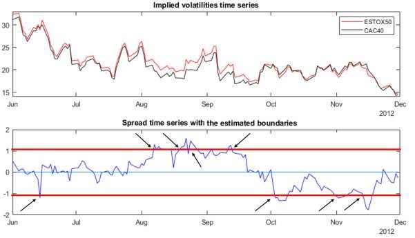
3.1 Estimation period
Using 1-year data, the following OLS regression is estimated:

 , = 0 + 1 , + (1)
where:

 - , is the implied volatility of the option written on Index observed at day 
 - , is the implied volatility of the option written on Index observed at day 
 - is the error term at time 
 - 0 is the intercept, that in this case simply acts as a scale parameter
 - 1 is the slope, measuring the linear relationship between the two implied volatilities
The estimate is performed for all possible pairs of indexes ( , ).
Notice that using IV, which are typically stationary time series, allows a correct measurement
of their association via OLS regression, as opposed to what happens when this approach is
applied to stock prices, which typically are (1) time series.

3.2 Trading period
Each estimation period is followed by a six-months trading period, in which a simple pair
trading strategy is implemented any time one of the options has an observed implied volatility
that sufficiently deviates from the predicted value based on the estimates of model (1). The
idea is that, when this divergence is detected, the agent could sell the relatively overpriced
option and buy the other one so as to close the position whenever the two volatilities align
again. If such a strategy is able to generate significant profits, the market efficiency in pricing
relative risks is actually disproved.
A definition of “sufficient deviation” is thus required. To this end, using the estimates of 0
and 1 obtained in the estimation period, we compute the Spread6 as:
 = , − ̂0 − ̂1 , (2)
The Spread is thus obtained as the out-of-sample residuals of model (1). Under stationarity of
both variables involved in the simple linear regression model, in-sample residuals are also a
stationary process, mean-reverting towards 0. We take advantage of this characteristic out-
of-sample and detect a “significant” deviation of , from its long-run value of 0, any
time the following relationship is violated:
 2 ̂ ≥ ≥ −2 ̂ (3)
where ̂ is the standard deviation of the residuals obtained in regression (1). All exits of the
Spread form these boundaries will be interpreted as a misalignment of the options’ implied
volatilities from their relationship as estimated in model (1), will be thus signaling a potentially
profitable mispricing, and will hence trigger a trading strategy. As an example, the top panel
of Figure 1 reports the time-series of the Implied Volatilities of one-month maturity ATM call
options written on CAC40 and ESTOX50 Indexes, which clearly share the same pattern. The

6
 This definition, including the estimated intercept, follows the one proposed by Vidyamurthy (2004).

 6

spread between these implied volatilities, along with its ±2 ̂ boundaries, are instead plotted
in the bottom panel: the trading is triggered very time the spread exists the boundaries, as
pointed by the arrows.

 Figure 1 - Example of implied volatilities and Spread time series

Notes: The top panel reports the time-series of the Implied Volatilities of one-month maturity ATM call options written on
CAC40 (black line) and ESTOX50 (red line) Indexes, between the 1st of July and the 31st of December 2012. The bottom panel
reports the estimated spread between these two implied volatilies (in blue) and ±2 ̂ boundaries (in red). The black arrows
indicate when the trading is triggered.

Consistently with the practice established in the pair-trading literature, we set up two types
of trading strategies: a “self-financing” strategy, in which the quantities traded in the two
stocks are such that no initial capital investment is required, and a “beta-arbitrage” strategy,
in which the quantities traded in the two stocks are determined as a function of the regression
slope estimates.
More specifically, if > 2 ̂, the option written on index is suspected to be
overpriced with respect to option written on index . Therefore, in the self-financing strategy,
one unit of option written on index is sold and at the same time the option written on is
bought in the amount affordable under the proceeds from the previous sale. In the beta-
arbitrage strategy, one unit of option written on is sold and the quantity bought of option
on equals to the amount bought in the self-financing strategy multiplied by ̂1 (the idea is
that the amount in euros spent for option written on X is equal to ̂1 times the price of option
Y). Both positions are then unwounded when the Spread reverts within the estimated
boundaries. Finally, all the open positions are forcibly closed when the end of the trading
period is reached or when the options get to maturity (to reduce the sensitivity of the results
to the natural decline of the options prices when approaching expiration, the positions are
closed two days before maturity).

 7

Conversely, if < −2 ̂, the option written on is suspected to be underpriced with
respect to the option written on , so that the trading scheme is exactly the opposite. In the
self-financing strategy, one unit of option written on is sold and with the proceeds from the
sale the affordable amount of option on is bought. In the beta-arbitrage strategy, one unit
of option on is sold and the quantity of option written on will be the same bought in the
self-financing strategy divided by ̂1. As above, all the positions are closed when the Spread
reverts within the estimated boundaries, or when the maturity of the option and/or the end
of the trading period is reached.
To reduce the sensitivity of our results to the natural decline of the options prices when
approaching expiration, all positions are forcibly closed two trading days before maturity.
Each transaction payoff and the final returns are computed once the initial trade is unwound
and will depend on the relative price of the traded options. Notice that returns can be
interpreted as excess returns only in the self-financing strategy since no initial investment in
needed. Instead, in the beta-arbitrage strategy the payoff when the trade is initiated depends
on ̂1 and affects the final outcome of the transaction.

 4. Empirical application
In this section we first present the dataset used and then the results obtained in terms of
profitability of the pair trading strategy described above.

 4.1 Data
The empirical application relies on daily data spanning the period from the 1st of May 2007
until the 31st of December 2017, for a total of 2784 days, and referring to five Stock Indexes
of the Euro Area, namely:

  CAC 40 (Cotation Assistée en Continu), quoted on the Paris Bourse;
  DAX 30 (Deutscher Aktienindex), quoted on the Frankfurt Stock Exchange;
  FTSE 100 (Financial Times Stock Exchange 100 index), quoted on the London Stock
 Exchange;
  FTSE MIB (Financial Times Stock Exchange Milano Indice di Borsa), quoted on the
 Milan Stock Exchange;
  ESTOX 50 (Euro STOXX 50): leading stock index for the Eurozone, covering 50 stocks
 from 11 Eurozone countries (Austria, Belgium, Finland, France, Germany, Ireland, Italy,
 Luxembourg, Netherlands, Portugal and Spain).
The advantage of focusing on options written on Indices is that, given that the underlying is a
synthetic representation of a stocks’ portfolio, the final payoff is cash-settled rather than paid
through an exchange of goods. Hence, no other transaction costs are incurred to cash-in the
payoff, aside from those strictly deriving from the trade.

 8

For each Index, we use the following data, all retrieved from Thomson Reuters DataStream7:

  Stock Index Prices;
  Options Prices of all the Call options written on the index, along with their maturities
 and strike prices8;
  Implied Volatilities of the at-the-money 1-month maturity Call Options written on the
 index.
For each day in the sample and for each underlying Index, we select the at-the-money (ATM
henceforth) call options. We focus on ATM options since most of their market value is related
to volatility, so that they are the most informative in this sense. This is very important for our
application since the long-run equilibrium relationship between pairs of options is established
directly through their (implied) volatilities.
Among the ATM options, we then select the one with the shortest maturity, since short-term-
maturity options are among the most liquid in the market. In doing so, we exclude those with
a residual life equal or less than 10 days, with the twofold aim to guarantee the possibility of
trading on that option and to reduce the sensitivity of the results to the natural decline of the
options prices when approaching expiration. This leaves us with ATM one-month options
whose time-to-maturity ranges between 11 days (corresponding to at least 7 trading days)
and 46 days (corresponding to at least 32 trading days).
Finally, we select the one whose strike price is as close as possible to the value of the
underlying Index. If two series are found to have the same absolute distance between strike
and Index price, we exclude the one with higher strike price, so as to maintain the one more
conservative in terms of final payoff.9
We thus end up, for each day in our sample, with one single ATM one-month call option for
each of the underlying indexes considered.10

7
 Through a deep analysis of the data and with the support of the data provider, many recording errors have
been corrected directly on Thomson Reuters DataStream. Most of such issues where due to the same
identification code being attributed to more than one series at different points in time.
8
 FTSE 100 call options prices are in pound sterling, while all others are quoted in euros. The corresponding daily
GB Sterling/Euro FX exchange rate is thus used to convert in euros the prices of options on FTSE 100. The
identifying number of each series is 6239 for CAC 40, 12158 for DAX 30, 11939 for ESTOX 50, 9501 for FTSE 100
and 7303 for FTSE MIB. In DataStream missing values on option prices are replaced with the previous day
observation.
9
 In the selection process, we further exclude all call options with non-standard maturity, i.e. with a maturity
settled in a different day from the third Friday of the month, as well as some calls presenting two series for the
same strike price. For these reasons, we excluded one option on the CAC 40, one option on the ESTOX 50 and
six options on the FTSE 100.
10
 Notice that the ATM one-month call option selected in a certain day, in which a trade is maybe opened, is not
necessarily the same ATM one-month call option selected in another day. This means that it might happen that
the call selected for the day a trading is opened does not coincide with the one selected for the day the same
trade is closed. Thus, in order to have the prices of the traded option in both the day in which the trade is
triggered and in the day in which the trade is closed, needed to compute the actual profits obtained trading an
option, we needed to store, for each selected option, the entire time-series of the prices. As a result, we actually
end up with 2784 (one for each day in our sample) option prices time-series.

 9

4.2 Preliminary analyses
The time series of the implied volatilities of one-month maturity ATM options written on the
selected Indexes are represented in Figure 2. Two major shocks are distinctly common to all
series, namely the outburst of the global Financial Crisis at the end of 2008 and the Sovereign
Debt Crisis at the end of 2011, both having brought instability (i.e. higher volatility) to the
European Financial Market. The series however share a very similar pattern also outside these
two extreme events, so the possibility of finding strong relationships between the IV of the
five underlying indexes seem quite high.

 Figure 2 – Implied Volatilies of the one-month ATM options, by underlying index.

 Note: The figure reports the time series of the Implied Volatility of the at-the-money 1-month
 maturity call options written on the following stock market indexes: CAC40, DAX 30, FTSE 100,
 FTSE MIB, ESTOX 50, from 1st of May 2007 until the 31st of December 2017.

The similarity of the Implied Volatilities across the five underlying indexes is further confirmed
by the degree of variability, which is very similar across the series (see panel A of Table 1) and
the quite high level of correlation (panel B of Table 1 - Descriptive statistics, correlation and
ADF test: one-month ATM options Implied Volatitlities, by underlying IndexTable 1), which
never falls below 0.75. 11

 Table 1 - Descriptive statistics, correlation and ADF test: one-month ATM options Implied Volatitlities, by
 underlying Index
 Panel A – Option Implied Volatilities
 CAC 40 DAX 30 ESTOX 50 FTSE 100 FTSE MIB

11
 In pairs trading applications the initial set of potential pairs is often artificially narrowed to highly correlate
(for instance, Miao, 2014, and Ammann & Herriger, 2002, pre-select pairs of stocks with correlation greater than
0.95). In our application none of the pairs has been excluded, thus avoiding the need of setting an arbitrary
threshold for correlation.

 10

Mean 21.59 21.14 22.23 17.75 24.98
 St. Deviation 8.95 8.70 8.85 8.91 8.30
 Min 8.34 9.05 8.84 4.62 10.36
 Median 19.65 19.11 20.32 15.40 23.04
 Max 90.74 89.41 78.49 91.41 76.24
 Panel B – Correlation across Option Implied Volatilities
 CAC 40 DAX 30 ESTOX 50 FTSE 100 FTSE MIB
 CAC 40 1 0.97 0.98 0.95 0.87
 DAX 30 1 0.97 0.94 0.86
 ESTOX 50 1 0.94 0.89
 FTSE 100 1 0.75
 FTSE MIB 1
 Panel C – ADF tests on Implied Volatilities
 CAC 40 DAX 30 ESTOX 50 FTSE 100 FTSE MIB
 ADF – with drift
 test statistics
 pvalue 0.0083
 ADF – with trend and drift
 test statistics
 pvalue

Notes: The table reports the main descriptive statistics for the Implied volatilities of one-month maturity ATM call options
over the entire sample period (panel A), the Pearson Correlation Coefficient across the Implied Volatilities (panel B), and the
t-statistics, and associated p-values, of the ADF test with drift only and with trend and drift, by underlying Index.

The Augmented Dickey-Fuller test for stationarity are then run on the implied volatilities. The
ADF was run setting a maximum lag length equal to 15 and with both drift-only and drift and
trend specifications. In all cases, the null for the presence of unit-root null is rejected a 95%
confidence level. The IV are thus stationary time-series highly correlated across each other
and apparently following a similar pattern over time, which we are going to exploit in the pair
trading statistical arbitrage. If such trading strategy is able to produce significant profits, then
EMH can be disproved.

 4.3 Main Results
Table 2 reports the results of the self-financing and the beta-arbitrage trading strategies,
implemented over the trading period spanning from the 1st of May 2008 until the 31st of
December 2017 (data from the 1st of May 2007 till 30th of April 2008 are used in the first
estimation period).
To begin with, the number of trades realized (column 13 of Table 2) is quite high, meaning
that during the sample period under analysis the spread kicked the estimated boundaries,
thus signaling potential mispricing on the market, in many occasions.12 The vast majority of

12
 These figures are cumulative across the six overlapping portfolios, so some trades might be double counted.
Yet, even assuming that all trades are common across the six portfolios, the overall number of suspected
mispricing would still be pretty high (equal to 11191/6 = 1865 trades). Considering that the trading days in our
sample are 2419 (2784 -365), this figure would suggest an average of nearly 1 trade every day (2419/1865=1.30).

 11

these trades(88%), which on average remain opened for 4 days, close because the Spread
reverts within the boundaries, while the rest are forcibly closed either because the options
involved in the trade expire (8%) or because the end of the trading period is reached (3%).
Despite the number of suspected mispricing is quite high, the average returns eventually
obtained implementing the self-financing strategy (which are directly interpreted as excess
returns since this strategy does not require initial investment) are indeed pretty low, on
average around 0.8%, and not statistically significant, as shown in column (1) of Table 2. The
corresponding extra-profit is equal to 9.30€, but again this is far from being statistically
significant. Dissecting the result by the pairs of underlying indexes on which the traded
options are written, we find that option pairs trading proved to be significantly profitable in
6 cases out of the 20 possible couples, with excess returns ranging from 4.3% (for the couple
FTSEMIB-CAC40, corresponding to 15.60 € in terms of average profit) to as much as 13.6%
(for the FTSEMIB-DAX30 couple, corresponding to an average profit of 56.60€). In all other
cases, the strategy does not provide significant returns, and in 4 cases it even leads to
statistically significant negative returns, all of which include the FTSE100, which points
towards the required exchange rate conversion in Euro as playing as an additional source of
friction.
The beta-arbitrage strategy differs from the self-financing strategy only in terms of traded
quantities, so that the number of transactions and the closure reasons are unaffected. Recall
however that, since in this case an initial investment is needed, the obtained returns cannot
be interpreted as excess returns. The average returns observed across all pairs are still
positive but much higher if compared to the one obtained implementing the self-financing
strategy (7.3% on average against 0.8%).13 Nonetheless, consistently with the results for the
self-financing strategy, the average return is not statistically significant. Moreover, looking at
the returns by pairs, statistically significant positive returns survive only for the pairs written
on FTSEMIB and on the ESTOX50.
All in all, despite the signals of potential mispricing are frequent, the statistical arbitrage does
not produce significant positive expected returns, leading to the conclusion that there is no
evidence against index option market efficiency. Notice that all the results presented so far
are computed without taking transaction costs into account. Their inclusion in fact is likely to
further reduce the profitability of the strategies, so our conclusion about index option market
efficiency is reached under the most conservative condition.

13
 The higher average return obtained is most likely due to the fact that the estimates obtained for beta are in
most of the cases very close to one. In the beta-arbitrage strategy, one unit of option written on is sold and
the quantity bought of option on equals to the amount affordable under the proceeds from the previous sale
multiplied by ̂1 . If the estimates of ̂1 is very close to one, this means that the initial investment is very close to
zero, which results in inflating the estimated final return.

 12

Table 2 – Results for the option pairs trading self-financing and beta-arbitarge strategies, by pairs of underlying indexes.

 Self-financing strategy Beta-arbitrage strategy returns Closing
 Average Total number
 Average NW Average Profits NW Average Average Profits Trading life of trades
 NW stat NW stat Boundary Maturity
 returns stat (or losses) stat returns (or losses) period end
 (1) (2) (3) (4) (5) (6) (7) (8) (9) (10) (11) (12) (13)
 CAC40-DAX30 0.003 0.18 3.77 1.21 -0.510 -0.97 6.01* 1.93 0.82 0.14 0.04 5.33 468
 CAC40-ESTOX50 -0.004 -0.64 -1.06** -2.19 -1.701 -1.31 -1.00** -2.13 0.97 0.02 0.01 2.60 525
 CAC40-FTSE100 -0.042** -2.59 -6.51*** -3.33 -0.834 -1.13 -6.25*** -3.08 0.86 0.09 0.05 4.31 538
 CAC40-FTSEMIB 0.044*** 3.46 31.02*** 4.21 0.733 1.30 23.12*** 2.81 0.88 0.08 0.04 3.99 560
 DAX30-CAC40 0.007 0.39 5.18* 1.85 0.484 0.36 5.90** 2.06 0.82 0.13 0.05 5.51 448
 DAX30-ESTOX50 0.005 0.40 1.35 0.89 -0.341 -0.50 2.89* 1.69 0.89 0.08 0.03 4.33 480
 DAX30-FTSE100 -0.022 -1.32 -5.91** -2.29 -0.256 -0.09 -6.42** -2.12 0.88 0.09 0.03 4.17 653
 DAX30-FTSEMIB 0.059*** 2.93 39.66*** 3.44 0.307 0.27 31.75** 2.62 0.85 0.11 0.04 4.72 570
 ESTOX50-CAC40 0.006 0.87 0.34 0.66 -0.973 -1.62 0.64 1.23 0.97 0.02 0.01 2.57 560
 ESTOX50-DAX30 0.023* 1.82 3.89** 2.23 -0.866 -0.94 6.34*** 3.18 0.84 0.12 0.04 4.81 504
 ESTOX50-FTSE100 -0.094*** -5.67 -12.34*** -5.95 -0.374 -1.47 -10.98*** -4.92 0.90 0.07 0.03 4.23 524
 ESTOX50-FTSEMIB 0.051*** 5.42 30.37*** 5.14 0.551** 2.70 28.17*** 3.97 0.92 0.05 0.03 3.58 683
 FTSE100-CAC40 -0.037** -1.85 -2.32 -1.10 -0.501 -0.89 -4.22** -2.01 0.83 0.12 0.05 4.74 507
 FTSE100-DAX30 -0.013 -0.86 -4.05 -1.61 0.013 0.03 -6.10** -2.31 0.86 0.10 0.04 4.22 747
 FTSE100-ESTOX50 -0.065*** -3.65 -4.70*** -2.86 2.328 0.95 -5.44*** -3.31 0.89 0.08 0.03 4.31 519
 FTSE100-FTSEMIB 0.008 0.32 16.64 1.21 -0.702* -1.87 6.03 0.41 0.84 0.12 0.05 4.69 597
 FTSEMIB-CAC40 0.043*** 3.49 15.60*** 2.96 0.192 0.61 15.55** 2.41 0.92 0.05 0.03 3.34 539
 FTSEMIB-DAX30 0.136*** 6.16 56.60*** 5.35 2.410 1.31 60.36*** 4.10 0.87 0.10 0.03 4.43 547
 FTSEMIB-ESTOX50 0.054*** 5.64 19.67*** 5.00 0.464** 2.67 22.86*** 4.49 0.94 0.03 0.03 3.05 683
 FTSEMIB-FTSE100 -0.024 -0.96 -9.77 -0.82 0.824 0.52 0.54 0.04 0.90 0.06 0.04 3.72 539
 ACROSS ALL PAIRS 0.008 0.02 9.30 0.06 0.073 0.00 8.78 0.05 0.88 0.08 0.03 4.09 11191
Notes: The table reports the results of the self-financing (columns 1 to 4) and beta-arbitrage (columns 5 to 8) pair trading strategies. For each strategy we report the average return and the
average profits (if positive) or losses (if negative), whose statistical significance is tested based on the Newey-West heteroskedasticity and autocorrelation robust t-statistics (Newey & West,
1987). The symbols ***, **, and * indicate significance at the 1%, 5%, and 10% levels, respectively. Columns 9 to 11 report the shares of trades closed due to the Spread reversion within the
boundaries, due to option expiration and due to having reached the end of the trading period, respectively. The last two columns report the average number of days the trades remained
opened, and the total number of trades observed. The results are reported by pairs of underlying indexes and refer to the trades triggered by the deviations of the spread estimated based on
the regression where the Implied Volatility of the option written on the first underlying Index is used as X and the Implied Volatility of the option written on the second as Y.

 13

4.4 Profitability drivers
We are interested in spotting the potential drivers of the profitability of index option pairs
trading. To this end, we regress the observed returns of the pairs trades on the characteristics
of both options involved in the trade, i.e. the one bought (long) and the one sold (short), and
on the overall condition of the financial market at the moment the trades took place. All
variables in the regression are measured at the moment the trade is closed.
The value of an option is function of several features, namely: moneyness, i.e. the closeness
between option strike price and price of the underlying asset; time to maturity, i.e. the time
left before expiration; the volatility of the underlying quotations; and, the interest rate. Since
the latter two are (supposed to be) common across all options traded in the market, we focus
on the time to maturity and the moneyness. The former is measured by the number of trading
days left before the option expires. The value of the option increases with the time left to
maturity, so the longer the maturity, the more (less) the chances of making a profit when a
long (short) position is taken. We thus expect the profitability of the pair trading strategy to
the positively associated with the maturity of the long option and negatively associated with
 
the one of the sold option. As for moneyness, we focus on the strike-price ratio, ( ), which
in our sample ranges in the interval [0.8 - 1.36] for the options sold and [0.85 - 1.62] for the
ones bought, with mean and median in both cases approximately equal to 1.14 We classify
each option as follows:
 
 ( ) < 0.98
 
 (4)
 ( ) > 1.02
 
 { ℎ 

Where is the strike of the option, is the underlying price (at the time the transaction
closes) and , , and denote the option being out-of-the-money, in-the-
money or at-the-money, respectively. Each trade involves two options, each of which at
closure can be in each of the three conditions of moneyness, resulting in 32 = 9 possible
combinations. In the regression we thus include 8 dummies capturing all the possible
combinations for the long and short options being, at the moment the trade is closed,
at-the-money, in-the-money, or out-of-the-money ( ), having the combination of both
options being ATM as reference category.15 Errore. L'origine riferimento non è stata trovata.
reports the distribution of the trades according to the moneyness of both options involved.

14 Notice that, even if the traded options are by construction both ATM when a position is opened, their
monenyness might well have changed at the time the position is closed (which is the moment the variables in
the regression refer to).
15
 We also tried alternative classifications, using as thresholds for ITM/OTM the mean value ± 0.01, 0.03, 0.04
and 0.05 and the results obtained (available upon request) remain qualitatively unchanged.

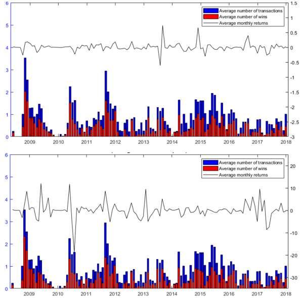
 14

Table 3 - Self-financing strategy transactions, by moneyness of the options involved
 Short leg
 Long leg
 IN ATM OUT
 IN 1895 413 14
 ATM 913 5793 518
 OUT 28 289 1328
 Notes: the table stratifies transactions based on
 the moneyness at the closure of the trade of each
 call option forming the pair, depending on the long
 or short positions taken on the asset.

In our empirical application, we work with call options, whose intrinsic value increases the
more the underlying price is higher than the strike price (i.e. the more strike-price ratio is
lower than 1). This means that the lower the strike-price ratio, the higher the chances of
making a profit when a long position is taken on a call and, symmetrically, the higher the
chances of losing if the call is sold. We thus expect the strategy returns to be positively related
with the bought option being ITM and the sold option being OTM. By the same token, we
expect the opposite this relation to be negative when short options are ITM and long options
are OTM.
 The profitability results of the implemented index option pair trading also shows a
remarkable variability across time (see Figure 3) 16. In order to assess if the profitability
significantly varies along with periods of financial turbulence, we also include a dummy
indicating if the trade is closed during one of the following crisis: the Financial Crisis (form
October 2007 to May 2009) and the Chinese stock market turbulence (from June 2015 to June
2016).

16
 The displayed results are obtained taking the average results, for each month of the trading period, of all the
trades occurred across all pairs.

 15

Figure 3 - Pairs trading (average) monthly results: trades, profitable trades and returns.

 Average results across pairs of the trading strategies implemented over the sample from May 2008 to December 2017:
 average number of transactions per month, average number of wins per month (i.e. trades with positive final payoff) and
 average monthly returns. The top panel refers to the results of the self-financing strategy, while the bottom one refers
 to the results obtained with the beta-arbitrage strategy.

following model:
 = 0 + 1 , ℎ + 2 , ℎ + (5)
 3 , ℎ , + 4 , ℎ , + 5 , ℎ , +
 6 , ℎ , + 7 , ℎ , + 8 , ℎ , +
 9 , ℎ , + 10 , ℎ , + 11 + 

where is the return realized on the (self-financing or beta-arbitrage) pair trading strategy
on trade , and , ℎ and , are the time to maturity of the option sold and bought,
respectively. The variables from , ℎ , to , ℎ , are dummies
capturing the moneyness of the options involved in trade (for instance, , ℎ , 

 16

takes value 1 if both options (long and short) involved in trade are in-the-money at the
 moment the trade was closed, and 0 otherwise). Finally, takes value 1 if trade is
 closed during the Financial Crisis or Chinese stock market turbulence as indicated above, and
 0 otherwise.
 Table 4 reports the estimates of various specifications of regression model (5) for both the
 self-financing and the beta-arbitrage strategies returns, using the entire sample of the
 realized trades. In most of the cases, the returns turn out to be significantly associated to the
 time to maturity of both the options involved (the only exception being specification (4), in
 which the estimated effect for both maturities is not distinguishable from 0). Moreover,
 consistently with expectations, the strategy returns are negatively associated to the time to
 maturity of the option sold and positively related to the maturity of the option bought. Not
 surprisingly, the estimates for the two sides of the trade are quite similar in terms of
 magnitude, which is not surprising given the standardized maturities of the options used in
 the sample. As for moneyness, the estimated effect is largely significant in most model
 specifications and explains most of the variability of the returns. Besides, in line with
 expectations, the strategy returns are on average higher whenever the option sold is OTM
 and/or the option on which a long position is taken is ITM, while on average lower when the
 sold option is ITM and/or the option bought is OTM. Finally, the estimated effect for the
 dummy suggests that the returns from pair trading strategy are significantly lower
 (and up to 5 percentage points lower) during periods of financial turbulence if compared to
 the entire sample average. Strikingly however, this difference is statistically significant only if
 referred to the extra-returns obtained applying the self-financing strategy.

 Table 4 – Drivers of the pair-trading returns.
 Self-financing strategy Beta-arbitrage strategy
 (1) (2) (3) (4) (5) (6) (7) (8)
 0.04*** 0.00 0.02*** 0.01 -0.03 -0.27 -0.05 -0.90
Constant
 (0.00) (0.70) (0.00) (0.15) (0.96) (0.50) (0.89) (0.24)
 -0.01*** 0.00 -1.13*** -0.89***
 , ℎ 
 (0.00) (0.55) (0.00) (0.00)
 0.01*** 0.00 1.14*** 0.92***
 , 
 (0.00) (0.54) (0.00) (0.00)
 0.02** 0.03*** 0.60 0.67
 , ℎ , 
 (0.03) (0.00) (0.46) (0.42)
 -0.38*** -0.38*** -5.38*** -5.34***
 , ℎ , 
 (0.00) (0.00) (0.00) (0.00)
 -1.05*** -1.07*** -25.34*** -18.60***
 , ℎ , 
 (0.00) (0.00) (0.00) (0.00)
 0.73*** 0.74*** 5.57 6.01
 , ℎ , 
 (0.00) (0.00) (0.50) (0.46)
 0.20*** 0.20*** 4.13*** 4.18***
 , ℎ , 
 (0.00) (0.00) (0.00) (0.00)
 0.02 0.03*** 0.94 1.05
 , ℎ , 
 (0.12) (0.00) (0.31) (0.28)
 0.77*** 0.78*** 13.49*** 13.68***
 , ℎ , 
 (0.00) (0.00) (0.00) (0.00)
 -0.15*** -0.14*** -2.29 -2.16
 , ℎ , 
 (0.00) (0.00) (0.22) (0.24)
 -0.02*** -0.05*** 0.43 -0.12
 
 (0.00) (0.00) (0.51) (0.86)
Ordinary R-squared 0.002 0.242 0.001 0.245 0.002 0.012 0.000 0.014

 17

Num. of observations 11191 11191 11191 11191 11191 11191 11191 11191
 Notes: The table reports the regression estimates for four alternative model specifications of equation (5),with p-values in
 parenthesis. The dependent variable is the return obtained implementing the pairs trading (self-financing or beta-arbitrage)
 strategy. is the time to maturity. is a dummy for the option being in-the-money, is a dummy for the option begin at-
 the-money and is a dummy for the option begin out-of-the-money, and they refer to both the option bought (long) and the
 option sold (short) in the transaction . is a dummy taking value 1 if trade closes during a period of financial turbulence.
 ∗significant at 10% level. ∗∗significant at 5% level. ∗∗∗significant at 1% level.

 In Table 5 – Drivers of the pair-trading returns: subsample of significantly positve returns.

 we repeat the analysis of profitability drivers focusing on the trades that actually produced
 significantly positive returns only. Despite the remarkably reduced subsample, the results are
 overall similar to the previous analysis, with the only difference that now time to maturity is
 no longer significant in any of the model specifications. Notice however that in both Table 4
 and Table 5 – Drivers of the pair-trading returns: subsample of significantly positve returns.

 the variables considered are not able to fully explain the strategy performance. Since also the
 price of the underlying and options volatility play a central role in determining transactions
 payoffs, we can conclude that profitability of options pairs trading is affected by much more
 factors than in case of application to the stock market and this may be the reason behind the
 variability of our results.
 Table 5 – Drivers of the pair-trading returns: subsample of significantly positve returns.
 Self-financing strategy Beta-arbitrage strategy
 (1) (2) (3) (4) (5) (6) (7) (8)
 0.07*** 0.01 0.04*** 0.04*** 0.35 0.31 0.55*** 0.05
 Constant
 (0.00) (0.37) (0.00) (0.00) (0.34) (0.15) (0.00) (0.90)
 -0.03* 0.00 0.01 0.02
 , ℎ 
 (0.09) (0.87) (0.65) (0.29)
 0.02 0.00 0.00 0.00
 , 
 (0.12) (0.82) (0.00) (0.00)
 0.07*** 0.07*** 0.34 0.43
 , ℎ , 
 (0.00) (0.00) (0.41) (0.31)
 -0.31*** -0.32*** -1.94*** -2.00***
 , ℎ , 
 (0.00) (0.00) (0.00) (0.00)
 -0.69*** -0.73*** 0.00 0.00
 , ℎ , 
 (0.00) (0.00) (0.00) (0.00)
 0.77*** 0.77*** 4.03 3.95
 , ℎ , 
 (0.00) (0.00) (0.29) (0.30)
 0.20*** 0.20*** 1.79** 1.68**
 , ℎ , 
 (0.00) (0.00) (0.01) (0.02)
 0.01 0.03* 0.91** 1.10**
 , ℎ , 
 (0.40) (0.05) (0.03) (0.01)
 0.71*** 0.71*** 2.53*** 2.62***
 , ℎ , 
 (0.00) (0.00) (0.00) (0.00)
 -0.12*** -0.11*** -1.23 -1.21
 , ℎ , 
 (0.00) (0.00) (0.22) (0.23)
 -0.03*** -0.06*** -0.11 -0.38
 
 (0.01) (0.00) (0.73) (0.23)
 Ordinary R-squared 0.004 0.212 0.001 0.217 0.000 0.030 0.000 0.032
 Num. of observations 5132 5132 5132 5132 1366 1366 1366 1366
 Notes: The table reports the regression estimates for four alternative model specifications of equation (5),with p-values in
 parenthesis. The dependent variable is the significantly positive return obtained implementing the pairs trading (self-financing or
 beta-arbitrage) strategy. is the time to maturity. is a dummy for the option being in-the-money, is a dummy for the

 18

option begin at-the-money and is a dummy for the option begin out-of-the-money, and they refer to both the option bought
(long) and the option sold (short) in the transaction . is a dummy taking value 1 if trade closes during a period of financial
turbulence. ∗significant at 10% level. ∗∗significant at 5% level. ∗∗∗significant at 1% level.

 5. Robustness
 In this section we check the robustness of our results. We first apply a stricter definition of
 reversion to the equilibrium, by having the positions closed whenever the Spread converges
 back to exactly 0 (or at the end of the trading period or when the options reach maturity),
 rather than just reentering within the estimated ±2σ ̂ boundaries, as in equation (3). Then, we
 address the potential concern that the relationship between implied volatilities, which we use
 to estimate the long-run equilibrium, might not be directly extended to options prices.

 5.1 Spread reaching the zero
 A stricter definition of convergence to equilibrium is applied, by closing the trades when the
 Spread reverts to zero, rather than just re-entering the boundaries. The results obtained in
 terms of profitability are reported in Table 6. As the condition for closing the trade is now
 much more restrictive, the average life is now much longer (on average 13 days compared to
 the 4 observed in the previous application). Moreover, the percentages of transactions closed
 due to options’ expiration or end of the trading period increase at the expense of a reduction
 in the closures coming from the Spread’s convergence to zero. Nonetheless, the total number
 of trades is even nearly halved and the option pair trading arbitrage strategy does not produce
 significant positive expected returns. Our main conclusion that the pairs’ trading strategy is
 not able to produce evidence against market efficiency remains thus unchanged. Similarly,
 the evidence concerning the profitability drivers, reported in Table 7 – Drivers of the pair-
 trading returns: closing when the Spread reaches 0.

 , remains qualitatively unchanged with respect to our baseline results.

 19

Table 6 – Results for the option pairs trading self-financing and beta-arbitarge strategies, by pairs of underlying indexes: closing when the Spread reaches 0.

 Self-financing strategy Beta-arbitrage strategy returns Closing Average Total number
 life of trades
 Average Average Profits NW Average Average Profits Trading
 NW stat NW stat NW stat Convergence Maturity
 returns (or losses) stat returns (or losses) period end
 (1) (2) (3) (4) (5) (6) (7) (8) (9) (10) (11) (12) (13)
 CAC40-DAX30 0.036 0.93 0.522 0.60 0.24 0.61 0.15 13.53 299
 CAC40-ESTOX50 -0.040* -1.81 -9.136** -1.97 0.40 0.50 0.09 11.02 309
 CAC40-FTSE100 -0.116** -2.52 -2.084* -1.94 0.45 0.43 0.13 11.83 336
 CAC40-FTSEMIB -0.009 -0.25 -0.480 -0.37 0.28 0.62 0.10 13.42 318
 DAX30-CAC40 0.031 0.96 1.316 1.15 0.20 0.64 0.16 14.67 278
 DAX30-ESTOX50 0.057* 1.94 5.137 1.03 0.28 0.60 0.12 13.77 309
 DAX30-FTSE100 -0.137*** -2.60 -1.203 -0.29 0.17 0.68 0.15 14.89 353
 DAX30-FTSEMIB 0.100* 1.80 -3.810 -0.78 0.20 0.66 0.14 13.75 319
 ESTOX50-CAC40 -0.047* -1.92 -4.643** -2.44 0.33 0.56 0.11 12.29 300
 ESTOX50-DAX30 0.079*** 2.76 0.227 0.28 0.18 0.68 0.14 14.26 307
 ESTOX50-FTSE100 -0.228*** -5.27 -1.935** -2.00 0.33 0.55 0.12 12.88 312
 ESTOX50-FTSEMIB 0.082** 2.11 0.519 0.74 0.28 0.60 0.12 13.30 354
 FTSE100-CAC40 -0.037 -0.81 1.202 0.56 0.39 0.49 0.13 12.51 317
 FTSE100-DAX30 -0.057 -1.27 -0.253 -0.17 0.16 0.69 0.15 15.04 386
 FTSE100-ESTOX50 -0.193*** -3.65 -9.652 -1.64 0.34 0.55 0.11 12.76 318
 FTSE100-FTSEMIB -0.030 -0.44 -0.348 -0.12 0.21 0.66 0.13 13.64 343
 FTSEMIB-CAC40 -0.017 -0.52 -0.699 -0.99 0.42 0.48 0.10 11.35 326
 FTSEMIB-DAX30 0.094* 1.74 1.269 1.21 0.26 0.62 0.13 12.81 343
 FTSEMIB-ESTOX50 0.109*** 2.73 2.556* 1.73 0.47 0.44 0.10 10.53 402
 FTSEMIB-FTSE100 -0.059 -0.82 0.983 0.26 0.31 0.56 0.13 11.92 311
 ACROSS ALL PAIRS -0.018 -0.02 -0.966 -0.02 0.29 0.58 0.13 13.00 6540
Notes: The table reports the results of the self-financing (columns 1 to 4) and beta-arbitrage (columns 5 to 8) pair trading strategies, whereby the trades close when the Spread reaches the zero level. For
each strategy we report the average return and the average profits (if positive) or losses (if negative), whose statistical significance is tested based on the Newey-West heteroskedasticity and autocorrelation
robust t-statistics (Newey & West, 1987). The symbols ***, **, and * indicate significance at the 1%, 5%, and 10% levels, respectively. Columns 9 to 11 report the shares of trades closed due to the Spread
reversion within the boundaries, due to option expiration and due to having reached the end of the trading period, respectively. The last two columns report the average number of days the trades remained
opened, and the total number of trades observed. The results are reported by pairs of underlying indexes and refer to the trades triggered by the deviations of the spread estimated based on the regression
where the Implied Volatility of the option written on the first underlying Index is used as X and the Implied Volatility of the option written on the second as Y.

 20

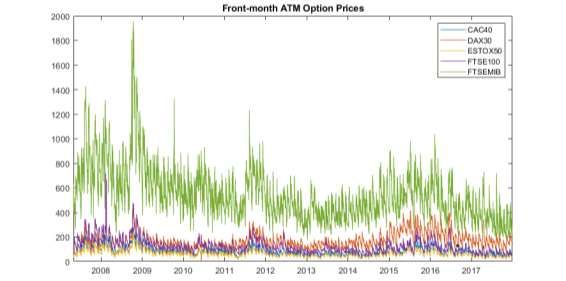
Table 7 – Drivers of the pair-trading returns: closing when the Spread reaches 0.
 Self-financing strategy Beta-arbitrage strategy
 (1) (2) (3) (4) (5) (6) (7) (8)
 0.00 0.03** 0.01 0.03** -1.82* -0.36 -1.24 -1.94
Constant
 (0.88) (0.04) (0.31) (0.04) (0.06) (0.80) (0.12) (0.24)
 0.00 -0.01 -0.02 -0.12
 , ℎ 
 (0.72) (0.39) (0.99) (0.91)
 0.00 0.01 0.10 0.24
 , 
 (0.84) (0.33) (0.92) (0.82)
 -0.11*** -0.10*** -4.42** -4.13**
 , ℎ , 
 (0.00) (0.00) (0.02) (0.03)
 -0.87*** -0.86*** -11.49*** -11.21***
 , ℎ , 
 (0.00) (0.00) (0.00) (0.00)
 -1.23*** -1.22*** -7.01 -6.56
 , ℎ , 
 (0.00) (0.00) (0.33) (0.36)
 0.98*** 1.01*** 18.67** 19.09**
 , ℎ , 
 (0.00) (0.00) (0.02) (0.01)
 0.28*** 0.29*** 7.72** 7.91**
 , ℎ , 
 (0.00) (0.00) (0.03) (0.02)
 -0.04** -0.02 0.48 0.41
 , ℎ , 
 (0.04) (0.37) (0.82) (0.85)
 1.23*** 1.23*** 20.46*** 21.17***
 , ℎ , 
 (0.00) (0.00) (0.00) (0.00)
 -0.37*** -0.37*** -3.04 -3.05
 , ℎ , 
 (0.00) (0.00) (0.37) (0.36)
 -0.11*** -0.09*** 1.01 0.79
 
 (0.00) (0.00) (0.51) (0.62)
Ordinary R-squared 0.001 0.400 0.004 0.403 0.000 0.018 0.000 0.018
 Num. of observations 6540 6540 6540 6540 6540 6540 6540 6540
Notes: The table reports the regression estimates for four alternative model specifications of equation (5),with p-values in
parenthesis. The dependent variable is the return obtained implementing the pairs trading (self-financing or beta-arbitrage)
strategy, closing the positions when the Spread reaches the value of 0. is the time to maturity. is a dummy for the option
being in-the-money, is a dummy for the option begin at-the-money and is a dummy for the option begin out-of-the-
money, and they refer to both the option bought (long) and the option sold (short) in the transaction . is a dummy taking
value 1 if trade closes during a period of financial turbulence. ∗significant at 10% level. ∗∗significant at 5% level. ∗∗∗significant
at 1% level.

 5.2 Spread estimated based on option prices
 In our baseline analysis each potential mispricing of options is spotted based on a long-run
 relationship estimated on options’ implied volatilities (rather than on underlying indexes’
 returns, as in Ammann and Herriger, 2002). Then, the statical arbitrate strategy is
 implemented on the options, using their prices to compute the final profits and returns. A
 potential concern with this approach might thus be that the long-run equilibrium relationship
 estimated on the implied volatilities might not directly translate to options prices. To address
 this concern we thus repeat the analysis estimating the long-run equilibrium relationship
 based on a(n artificially derived) time series of options prices (OP here on).
 More specifically, for each underlying index the corresponding OP time series is obtained
 collecting, for each trading day, the price of the option that is at-the-money and front-month
 at that point in time. Errore. L'origine riferimento non è stata trovata. and Table 8 report a
 graphical representation and the main descriptive statistics of the OP time-series obtained.
 Despite the degree of correlation is generally lower compared to the series of the implied
 volatilities, the association is still relevant, ranging between 0.56 to as high as 0.95 (see Panel
 21