An Inchworm-Inspired Motion Strategy for Robotic Swarms

This article has been published in a revised form in Robotica [https://www.doi.org/10.1017/S0263574721000321]. This version
 is free to view and download for private research and study only. Not for re-distribution, re-sale or use in derivative works.
 © Cambridge University Press.

An Inchworm-Inspired Motion Strategy for
Robotic Swarms
Kasra Eshaghi*ψ, Zendai Kashinoψ, Hyun
Joong Yoonϕ, Goldie Nejatψ, Beno Benhabibψ
ψ Department of Mechanical and Industrial Engineering, University of Toronto, 5 King’s
College Road, Toronto, ON, M5S 3G8, Canada.
Φ School of Mechanical and Automotive Engineering, Daegu Catholic University,
Hayang, Gyeongsan, Gyeongbuk 712-702, Republic of Korea
E-mails: kasra.eshaghi@mail.utoronto.ca, zendkash@mie.utoronto.ca, yoon@cu.ac.kr,
nejat@mie.utoronto.ca, benhabib@mie.utoronto.ca
(Accepted __, First published online: __)
SUMMARY
Effective motion planning and localization are necessary tasks for swarm robotic systems to maintain
a desired formation while maneuvering. Herein, we present an inchworm-inspired strategy that
addresses both these tasks concurrently by using anchor robots. The proposed strategy is novel as, by
dynamically and optimally selecting the anchor robots, it allows the swarm to maximize its
localization performance while also considering secondary objectives, such as the swarm’s speed. A
complementary novel method for swarm localization, that fuses inter-robot proximity measurements
and motion commands, is also presented. Numerous simulated and physical experimental examples
are included to illustrate our contributions.
KEYWORDS: Swarm Robotics; Motion Planning; Swarm Localization; Millirobots, Multi-
Robot Systems.
1. Introduction
 Research on swarm robotic systems (SRSs), typically, refers to the study of autonomous teams
that act as a single entity to achieve objectives that are beyond the capabilities of their individual
members.1-7 Inspired by biological swarms, they are characterized by their high degree of inter-robot
coordination and the large number of member robots, employing decentralized, semi-centralized, or
centralized control architectures.8-11 Correspondingly, such swarm systems, often, balance desirable
properties associated with decentralized architectures (e.g., scalability to larger teams and robustness
to the loss of members) with the relative simplicity of centralized control. In academia, SRSs are,
commonly, investigated using millimeter scale robots, millirobots.12-14
 An essential element in utilizing SRSs is the planning and control of their motion, which is often
termed as formation control.15 This process primarily involves the planning and controlling the motion
of the individual member robots, while the overall swarm travels along a specified trajectory. Swarm
localization, (i.e., determining the position of all swarm members), in this context, is important,
especially, as localization errors directly translate to errors in motion commands and ineffective
formation control. Past research has dealt with these issues (i.e., motion planning and localization),
mostly, separately – in contrast to our research discussed herein that deals with both issues
concurrently.
 Approaches to swarm-motion planning, commonly, assume that member robots move from an
initial formation to a destination one without an overall ‘swarm-shape’ (geometry/ configuration)
control along a trajectory. They, typically, employ a decoupled two-phased approach: (i) planning the
trajectories of the robots individually, and (ii) incorporating a separate coordination mechanism to

* Corresponding author. Email: kasra.eshaghi@mail.utoronto.ca

2 An inchworm-inspired motion strategy for robotic swarms

ensure inter-robot collisions are avoided.16-20 Methods that do consider maintaining a desired
swarm formation, while following a trajectory, on the other hand, are, typically, categorized as
behavioral,21-24 leader-follower,25-28 or virtual-structure methods.15,29,30 However, these
approaches are subjected to a variety of constraints on formation as well as trajectory following.
Other approaches to swarm-motion planning have, for example, investigated methods for area
coverage and monitoring,31,32 and collision free paths in real time.33
 Approaches to swarm localization, mainly, focus on estimating the relative distances between
robots,12-14,34,35 or estimating the changes to the swarm’s formation by using sample statistics from
the swarm.36-39 Methods of estimating the positions and orientations (poses) of all robots in the
swarm by fusing sensing data and motion commands,40-45 and methods that propose the use of
external infrastructure, such as stationary beacons46-49 (e.g., GPS, NorthStar) and computer vision
systems50-52 (e.g., AprilTag, WhyCon, OptiTrack) have also been suggested in the literature. The
latter ones tend to be more accurate, as the use of external infrastructure would yield the same
level of uncertainty independent of travelled distance. However, often, external infrastructure may
not be readily available to assist with localization (e.g., in disaster zones) or even possible to use
(e.g., unstructured indoor environments). External infrastructures may also require additional
hardware to be installed on the swarm robots – a difficult task due to the size limitations of
millirobots used in swarm robotics research12-14.
 The few hybrid approaches to swarm-motion planning that also consider localization, typically,
advocate the use of anchor robots.53-57 Anchors represent robots that remain stationary, while other
mobile units move to their destination. Use of anchors may improve the localization accuracy of
the swarm as they provide stationary references (i.e., landmarks) that can be detected by other
robots. In the methods discussed in refs. [53-55], the robots implement a leap-frogging strategy,
where the robots take turns moving toward their destinations. These approaches select intermediate
goal positions for the robots that maximize localization accuracy,53,54 or plan robot paths that
minimize the accumulated uncertainty in localization.55 However, commonly, these have been
developed for smaller teams of three to four robots and their formulation may not be scalable to
larger swarms.
 A method for localizing larger swarms was proposed in ref. [56], where robots move to their
destination one at a time and update their respective estimated pose after each movement. This
update fuses inter-robot proximity measurements, the estimated location of anchor robots, and the
(single) mobile robot’s motion command through an Extended-Kalman-Filter (EKF). The method
presented in ref. [57] is, similarly, scalable to larger swarms. In the method, the swarm is randomly
divided into two equal-sized subgroups that take turns in acting as anchors. After a predetermined
time, all robots stop to localize themselves by fusing measurements to selected nearby anchors and
are provided the next set of motion commands. The subgroups, then, switch roles. This two-step
motion strategy, however, requires the team to be divided into subgroups prior to deployment,
thus, preventing the swarm from selecting anchors dynamically. This method also suggests that
subgroups switch roles based on a pre-determined time interval (i.e., it requires robots to use a
synchronized clock). Furthermore, it is assumed that all mobile robots can ‘see’ all anchors.
 Herein, we propose an inchworm-inspired motion-planning strategy for swarm trajectory
following that employs dynamic anchor selection. Beyond past methods that use anchors in stricter
roles, our novel strategy allows (a) the balancing of swarm-motion speed versus accuracy per
users’ needs (i.e., flexibility), and (b) the use of any localization method (i.e., modularity).
 In contrast to methods that limit the robots to moving one at a time or, for example, through
two-grouped motion, our proposed strategy achieves flexibility by allowing the swarm to
dynamically select the number and choice of robots that act as anchors. In addition to meeting a
motion-speed versus accuracy requirement, adjusting the choice of anchors also allows the swarm
to meet run-time practical constraints, such as the finite communication range between robots.

An inchworm-inspired motion strategy for robotic swarms 3

 Abovementioned modularity is achieved by decoupling the two main problems at hand – i.e.,
determining (i) an effective swarm-motion planning strategy, and (ii) an accurate global swarm-
localization method. It is conjectured that accurate swarm motion can only be achieved via accurate
global localization. The work presented herein, also, marks one of the first swarm-motion planning
strategies designed to work with any localization method.
 A complementary novel localization method that efficiently and effectively fuses local swarm-
formation estimates with motion information to localize the swarm in a global reference frame is also
presented herein. In contrast to earlier approaches, this localization method does not require direct
interactions between (all) the mobile and anchor robots. Namely, it can localize the swarm with partial
information acquired from robots regarding their respective neighbors, as first discussed in our work
reported in ref. [45].

2. Problem Definition
The objective of our study is to develop an effective motion-planning strategy for a swarm of 
 
Robots, = { } =1 , as it travels along a desired trajectory, defined by a time-phased set of (swarm)
configurations – a point-to-point (PTP) trajectory, Fig. 1 below.
 In imitating an inchworm, the motion-planning sub-strategy to be developed would move the
swarm between any two successive configurations (i.e., points in PTP motion), Fig. 1, through
multiple intermediate steps. In each intermediate step, some members of the swarm, designated as
anchor robots, would remain stationary, while others, designated as mobile robots, would travel to
the next desired configuration.
 As discussed earlier in the Introduction, and illustrated in our investigations, a key variable in an
inchworm-inspired sub-strategy is the selection of anchors for every incremental step – namely, the
selection of both the number of anchors, , as well as the choice of anchor robots, . It is
conjectured that such selections would have a tangible impact on the performance of an inchworm
motion, especially, for accurate trajectory tracking. A primary problem addressed in this paper is,
thus, the optimal selection of anchors during runtime.
 Effective swarm trajectory following, with high fidelity, is also conjectured to depend on accurate
localization during runtime. However, one must note that, localization performance for swarms that
utilize inchworm-type trajectory following would be directly affected by the speed requirement for
the task at hand. Namely, the faster the speed of the swarm, the lower number of anchor robots that
can be used by the inchworm motion sub-strategy, thus, resulting in reduced localization and motion
accuracy. This presents us with a dilemma: one would like to have higher number of anchors for better
motion accuracy, though this would come at a price of slower motion.

 Start configuration Desired configurations

Fig. 1. PTP trajectory swarm motion.

4 An inchworm-inspired motion strategy for robotic swarms

 The abovementioned two issues are closely interdependent and need to be treated concurrently.
In this context, a measure of swarm speed performance, , is first defined herein by:
 ( )
 ( ) = 
 , (1)

where ( ), is a representation of the achievable speed of a swarm operating with anchors,
normalized with respect to a representation of the maximum speed achievable by the swarm with no
anchors, .
 Similarly, a measure of swarm localization performance, , is defined by:
 ( , )
 ( , ) = , 
 , (2)

where ( , ) is the localization error for a swarm operating with a specific selection of anchor
robots, ( , ), normalized with respect to the worst-case localization error of the swarm with no
anchors, , .
 In this work, thus, we propose that, anchor selection for the proposed inchworm sub-strategy
should aim to maximize an overall swarm motion performance metric, , defined by:
Maximize:
 ( , ) = ( ) − ( , ), (3)
subject to:
 ( , ) ≤ 0
 , (4)
 ℎ( , ) = 0
where and are weights denoting the importance of the swarm speed and localization
performance, ( + = 1), and, ( , ) and ℎ( , ) represent swarm motion constraints
(e.g., connectivity, speed, and desired configuration feasibility).
 One can recall that Eq. (3) needs to be solved in an online manner. Furthermore, in addition, the
swarm-localization process also needs to be formulated for runtime solution with potentially limited
measurement data.

3. Overview of Proposed Swarm-Motion Strategy
As described above, the objective of our study is to develop an effective motion-planning strategy for
a swarm to travel along a desired trajectory, defined by a time-phased set of (swarm) configurations
– a point-to-point (PTP) trajectory, Fig. 1. In this context, the inchworm-inspired motion sub-strategy
moves the swarm between two successive configurations, as part of the desired PTP trajectory, over
multiple incremental steps. The inchworm sub-strategy (a) dynamically selects the optimal anchor
robots for each successive move between two desired configurations in order to maximize the swarm’s
overall motion performance, detailed in Section 4 below, and (b) it also re-estimates the swarm
configuration after every incremental move of the inchworm motion, detailed in Section 5 below.
Continuous repetition of the inchworm-inspired motion sub-strategy allows the swarm to follow the
desired PTP trajectory.
 An overview of the proposed inchworm sub-strategy between two successive configurations, in
the context of PTP swarm motion, is presented in Fig. 2 below. In this figure and onward, in this
paper, any swarm configuration, , is defined as the set of all global robot positions (in the swarm):
 
 = { } =1
 
 , (5)

where = ( , ) represents the position of Robot i with respect to the global reference frame,
 .

An inchworm-inspired motion strategy for robotic swarms 5

 Current configuration, 
 Desired configuration, 

 Select optimal anchor robots , 

 =1

 Calculate first set of motion commands 1

 Move mobile robots, , based on latest motion
 commands, , while anchors, , remain stationary

 Calculate updated motion
 commands Re-localize the swarm ̂ 

 = +1 Is < ?
 Yes
 No

 = ̂ 
Fig. 2. The proposed swarm-motion strategy in the context of swarm-motion execution.

 In Fig. 2 above, for a given ‘couple’ of successive configurations, i.e., the swarm’s (first) current
and (next) desired configurations, and , respectively, the proposed inchworm sub-strategy:
 (i) Selects the optimal set of anchor robots, ( , )*, to use in all the steps of the incremental
 (iterative) motion toward , and, consequently, determines the necessary number of steps to
 move the swarm from to , ;
 Sets iteration/step number = 1;
 (ii) Calculates the motion commands for the (first) set of mobile robots, based on and , 1;
 (iii) Moves (only) the mobile robots, for the iteration at hand, , to their destination on , based
 on the latest motion commands, , while the anchors, , remain stationary – it must be
 noted that would only be achieved in approximation due to a multitude of errors (including
 robot motion errors);
 (iv) Re-localizes the swarm, after the motion of all the mobile robots has been completed, and
 obtains an estimate of the latest (true) swarm configuration (filled dots in Fig. 3(b)-(d)), ̂ ;
 If there are remaining mobile robots to move, i.e., < , sets iteration number = + 1 and
 continues to (v) below, otherwise, sets = ̂ and exits the loop.
 (v) Re-calculates the motion commands for the next set of mobile robots based on and the latest
 ̂ , and returns to (iii) above.
 It can be noted that the optimal anchor selection step of the proposed swarm-motion strategy is
completed in a centralized manner. The remaining components, which include the calculation and
execution of motion commands, and the necessary steps for re-localization, however, can be
completed in a decentralized manner to promote scalability and robustness.

6 An inchworm-inspired motion strategy for robotic swarms

 1 1

 1
 (a) (b)
 
 (c) (d)
Fig. 3. The proposed inchworm-motion sub-strategy: (a) current and desired configurations, , , (b)-(d)
intermediate estimated swarm configurations (filled circles), ̂ for steps = 1, 2, 3, respectively.

 The proposed inchworm sub-strategy is illustrated in Fig. 3 above, for a swarm of three robots,
with one mobile robot at a time. The motion strategy is novel in that it allows the swarm to
dynamically select the (number and choice of) anchor robots as it travels through a sequence of
configurations. This (flexibility) feature is used herein to maximize the motion performance (speed
and localization) of the swarm, Eq. (3). One can note that dynamic anchor selection could also
facilitate the consideration of other objectives, including, for example, maintenance of a desired
degree of connectivity in the swarm. Additionally, repeatedly estimating the intermediate
configurations of the swarm allows us to enhance the estimated position of anchor robots and, as a
result, provide more accurate motion commands.

4. Proposed Inchworm-Motion Sub-Strategy
The inchworm-motion sub-strategy outlined above requires the dynamic selection of optimal anchor
robots for every step of (multi-step) motion between two successive swarm configurations. Herein,
we present a novel search method which determines ( , )* that maximize the swarm’s motion
performance, Eq. (3), as it moves from to .
4.1. Optimization metrics for anchor selection
In Eq. (1), for the proposed inchworm-motion sub-strategy, the swarm’s speed can be represented as
the inverse of the number of steps required to reach to desired configuration, :
 1
 ( ) = , (6)
 ( )
where
 
 ( ) = . (7)
 − 

As per Eq. (6), the maximum achievable swarm speed corresponds to a swarm operating with zero
anchors (i.e., = 0, = (0) = 1). It should also be noted that only anchor numbers that result
in an integer number of incremental motion steps, , are considered feasible. For example, for a
swarm of = 10 robots, the feasible number of anchors would be = 0, 5, 8, or 9.
 The localization error of the swarm for a given choice of anchors, in turn, can be defined as the
mean distance between the true and estimated positions of all robots once all robots have reached 
(i.e., all steps are completed):

An inchworm-inspired motion strategy for robotic swarms 7

 1
 
 ( , ) = ∑ =1 ̂ |,
 | − (8)
 
where and ̂ are the true and estimated positions of Robot i in Configurations and
 ̂
 , respectively. It is important to clarify that, in our simulations, is calculated based on the
noisy motion of the individual robots, whereas ̂ is an estimate of this (localized) swarm
configuration, after the last step, using the proximity sensors on the individual robots.
 A thorough investigation into anchor selection, which included extensive simulated experiments,
verified that the number and choice of anchors have a meaningful impact on swarm-motion speed and
post-movement localization accuracy, Eq. (6) and Eq. (8), respectively. These investigations have
also indicated that the worst-case localization error would correspond to a swarm operating with no
anchors (i.e., = 0, , = (0, ∅)). The results of these investigations are summarized below.

4.1.1. Effect of the Number of Anchors. In this paper, it is conjectured that the number of anchors
affects both the speed and localization performance of the swarm. With a greater number of anchors,
fewer mobile robots can move at any one time and the swarm must go through more steps to reach
the desired configuration. As noted above, the swarm’s speed can be represented as the inverse of the
number of steps required to completely move the swarm to a desired configuration, Eq. (6). This
representation suggests that the swarm’s speed and, thus, its corresponding performance, , decreases
linearly with increased number of anchors. Furthermore, the maximum achievable speed of the swarm
corresponds to one’s operating with no anchors.
 Regarding swarm localization performance, extensive series of simulations were conducted. In
these, a swarm of robots was instructed to move from one (same) starting configuration, , to
another (random) desired configuration, , using the proposed inchworm motion strategy. For each
incremental motion step, a fixed number of robots were designated as anchors while the other
robots moved directly and concurrently to their next destination. Once the inchworm motion was
completed, noisy sensor measurements were simulated and used to estimate the swarm’s
configuration. For each motion simulation experiment, a swarm localization error, ( , ) was,
then, calculated through Eq. (8).
 1,000 random experiments were simulated for a swarm size of = 10 robots. Fig. 4(a)-(d) below
show the localization error obtained for cases with (a) zero, (b) five, (c) eight, and (d) nine anchors,
respectively. All simulations were subjected to different levels of noise in their inter-robot sensing
and motion-command executions. The results are plotted as localization error versus average distance
traveled by the robots in the swarm.
 The simulation results indicate that an increase in the number of anchors reduces localization error,
though, sub-linearly (i.e., there are diminishing returns to designating more robots as anchors). The
results also show that the worst-case localization error corresponds to the swarm that is operating
without the use of anchor robots (i.e., , = (0, ∅))

 (a) (b) (c) (d)

 Fig. 4. Swarm localization errors for (a) zero, (b) five, (c) eight, and (d) nine anchors, respectively.

8 An inchworm-inspired motion strategy for robotic swarms

4.1.2. Effect of the Choice of Anchors. It is further conjectured, herein, that the specific choice of
anchors does not have a tangible impact on the speed of the swarm, though, it could affect localization.
A series of simulated experiments was, thus, conducted to validate the conjecture that the choice of
anchors indeed has an impact on swarm-localization performance. In this set of experiments, random
desired configurations were generated. Then, for each random desired configuration, corresponding
swarm inchworm motion was simulated for all possible combinatoric choices of anchors for a fixed
 . The results of simulated motion and the subsequent estimations were evaluated in terms of the
localization error, ( , ), Eq. (8).
 1,000 random experiments were simulated for a swarm size of = 10 robots, where = 5
robots remain stationary at a time. For such a case, there exist a total of 252 possible 5-robot anchor
selections. All simulations were initialized with the same uncertain estimate of the swarm’s initial
configuration, . All simulations were also subjected to different levels of noise in their inter-robot
sensing and motion command executions.
 Fig. 5(a)-(d) below show the localization errors for the (a) no anchors, (b) random anchors, (c)
global worst anchors, and (d) global best anchors cases, respectively. The results are plotted as
localization error versus average distance traveled by the robots in the swarm. A global worst/best
represent the results of the choice of anchors that achieved the highest/lowest localization error for a
given desired configuration, respectively. Moreover, random anchors represent the localization error
associated with a choice of anchors that was selected randomly from the 252 possible choices. The
results indicate that, for a given set of possible anchors, there exists an optimal sub-set to choose from
that would result in the minimum possible localization error, ( ).

 (a) (b) (c) (d)
 Fig. 5. Swarm localization errors for different combinations of anchors: (a) zero anchors, (b) random anchors,
 (c) global worst anchors, and (d) global best anchors.

4.2. Search algorithm
The proposed search algorithm for ( , )* comprises two nested loops, Fig. 6 below. Assuming
knowledge of the swarm’s initial (pre-motion) configuration, , the search begins by, first,
determining and , . Then, the outer optimization loop (Fig. 6, red dashed line) seeks the
optimal number and choice of anchors by searching through the space of all feasible number of anchor
robots. The inner loop (Fig. 6, blue dashed line), in turn, determines the best choices of anchors for
 considered by the outer loop.
4.2.1. Outer optimization loop. Determination of the optimal number of anchors, could be
conducted by searching through the space of all feasible numbers using a simple (single, discrete-
variable) search engine. For a (feasible) number of anchors considered in this outer loop, the
corresponding optimal choices of anchors, ( ), would, then, be determined through the inner
optimization loop described below.
 One must note that the expected localization error of the swarm with any number of anchors at
hand, ( , ( )), would also be returned from the inner loop. This measure would, then, be used
in Eq. (3) to calculate the swarm’s overall motion performance for the number of anchors considered
in this outer loop, to eventually determine the final set of optimal anchors, ( , )*.

An inchworm-inspired motion strategy for robotic swarms 9

 Current configuration, 
 Desired configuration, 

 Calculate motion performance for = 0
 0, ∅ , , , 

 Select feasible 

 Update 

 Is feasible?

 No Yes

 Determine optimal anchors for ( ), , 
 /

 Calculate motion performance for , 

 Stopping criterion
 No achieved?

 Yes

 Optimal anchor selection, , 
Fig. 6. The proposed optimal anchor robot selection method.

4.2.2. Inner optimization loop. For every feasible number of anchors considered, , a search is
carried out to determine the corresponding choice of anchors that yield minimum localization error.
Namely, the inner optimization loop solves for:
 ( ) = arg min ( , ( )). (9)
 ( )

 Calculating the expected localization error for a given number and choice of anchors,
 ( , ( )), consists of simulating the inchworm motion, and computing the localization error
once all robots execute their movement commands. All steps of the simulated inchworm motion,
which include intermediate localization, are perturbed with noisy motion and proximity
measurements to represent a realistic scenario.
 One must note that the optimization problem at hand, Eq. (9), is an NP-hard combinatoric
optimization problem with possible solutions numbering:
 
 −1 − 
 = ∏ =0 ( ), (10)
 
where is the number of mobile robots for each step of motion ( = − ). It is, thus,
recommended to use a combinatoric optimization method, such as a variation of the genetic algorithm,
to guide which anchor choices to evaluate in this inner optimization loop. Furthermore, it is
recommended to seed the search engine with high-quality initial solutions to expedite the
optimization. A heuristic to produce one such high-quality initial solution, developed through our
work, is proposed below.

10 An inchworm-inspired motion strategy for robotic swarms

4.2.3. Proposed Heuristic for Initial-Guess Selection. An initial guess of anchor robots can be chosen
based on a variety of heuristics. Herein, we conjecture that the optimal choice of anchors for each
incremental step towards the desired configuration is dependent on the underlying characteristics of
the swarm’s post-motion configuration.
 In this regard, we propose two measures that encapsulate such characteristics: the expected
distribution of the anchor robots, and the expected separation between the anchor and mobile robots.
Namely, it is expected that the choice of anchors that maximize distribution and minimize separation
in the post-motion configuration would result in relatively high localization accuracy. This heuristic
was developed based on the proposed localization method used for the simulations in Section 4.1.
Analysis of this method, detailed in Section 5 below, indicates that maximizing distribution and
minimizing separation could maximize the influence of anchor robots and allow the swarm to achieve
reduced localization errors.
 A swarm’s distribution is a measure of the area covered by the anchor robots. The swarm
distribution, , after k steps of the inchworm sub-strategy, can be defined as the average distance
from the centroid of all anchor robots to all the individual anchors:
 1
 ̂ − ̅
 ( ) = ∑ ∈ (| ̂ |),
 (11)
 
where are all anchor robots for the kth step, and ̅
 ̂ is the estimated centroid of these anchors.
 
 A swarm’s separation, conversely, is used to capture the connectivity between anchor and mobile
robots. Separation, , after k steps of the inchworm sub-strategy, can be defined as the difference
between the centroid of the cluster of anchor robots and the centroid of the cluster of mobile robots:
 ̅
 ( ) = | 
 ̂ ̅
 ̂
 − |, (12)

where, ̅ ̂ is the centroid of the mobile robots used in the kth step of the inchworm sub-strategy.
 
For this initial heuristic, the position of mobile robots is calculated based on their provided motion
commands.
 The heuristic proposed for determining a high-quality initial solution for each step is, thus:
Maximize:
 1
 ( ) = ( ) + . (13)
 ( )

 Results of extensive series of simulations in our work, as will be detailed in Appendix A, illustrated
that anchors determined through the proposed heuristic would outperform random choices that can be
used as an initial guess.

5. Proposed Swarm-Localization Method
The proposed inchworm motion sub-strategy requires the swarm’s configuration to be re-estimated
after each incremental step, Section 3. Herein, we present a novel localization method that obtains an
estimate of the swarm’s configuration, ̂ , by fusing an estimate of the swarm’s (true) configuration,
obtained based on motion commands, , ̂ , with an estimate of the swarm’s topology, obtained
based on inter-robot proximity measurements, ̂ . For simplicity, the index k is omitted in the
following description of the localization method.
 A swarm topology, as noted above, defines the positions of all the robots with respect to a local
swarm frame, , Fig. 7 below:
 
 = { } =1
 
 . (14)

An inchworm-inspired motion strategy for robotic swarms 11

 1 
 1
 
 1

Fig. 7. Swarm topology.

As shown in Fig. 7 above, the swarm’s topology can be related to its configuration through the pose
of the local swarm frame with respect to the global frame, , ( , ). Namely, the position of
Robot i with respect to can be transformed to through:

 ( , , ) = + ( ) , (15)

where ( ) is the rotation matrix corresponding to the orientation of with respect to :
 cos( ) − sin( )
 ( ) = [ ]. (16)
 sin( ) cos( )

 Fig. 8 below presents an overview of the proposed two-phase localization method. Estimates of
the swarm’s configuration and topology are acquired in Phase 1 and subsequently fused in Phase 2.
 The proposed localization method detailed below is novel in that it does not require direct
interactions between all mobile and anchor robots. As long as the post-motion swarm configuration
remains connected (i.e., each robot can be sensed by at least one neighbor), the described method is
applicable. This feature simplifies swarm trajectory planning and control, as the required degree of
swarm-connectivity constraint is lower than would be for other localization methods. It must also be
noted that, although the proposed localization method was developed, primarily, for our inchworm
swarm-motion strategy, it would, certainly, be usable by all robotic swarms equipped with the
necessary sensing technology.

 Pre-motion estimated configuration, ̂ 0
 Phase 1 – Data acquisition

 Desired configuration, 

 Estimate swarm configuration based on motion commands ̂ 
 /
 Acquire inter-robot proximity measurements, { , ∈ 1, , }

 Estimate swarm topology ̂ 

 Phase 2 – Data fusion

 Estimated swarm configuration, ̂ 

Fig. 8. The proposed swarm-localization method.

12 An inchworm-inspired motion strategy for robotic swarms

5.1. Phase 1 – Data acquisition
In Phase 1, (1) a preliminary configuration estimate, in the global (motion) frame, , and (2) a
topology estimate, in the local (swarm) frame, , are obtained independently.
5.1.1. Phase 1.1: Preliminary swarm-configuration estimation. A preliminary estimate of the swarm’s
configuration, after an incremental step of the inchworm sub-strategy, can be determined by assuming
the motion commands of the mobile robots were executed with no uncertainty. A vector representing
the change in position of Robot i, ̂ , is used in our formulation. Since it is assumed that no odometry
is available, this vector represents the difference between Robot i’s desired position, , and pre-
motion estimated position, ̂ 0 , respectively. For the mobile robots :

 ̂ = − 
 ̂ 0 , ∈ , (17)
whereas, for anchor robots, :
 ̂ = 0, ∈ ,
 (18)
 
A preliminary estimate of the post-motion configuration of the swarm, ̂ = { 
 ̂ } =1, can, then,
be acquired by applying the above defined motion commands:
 ̂ = 
 ̂ 0 + 
 ̂ , ∈ {1, , }. (19)
Fig. 9 below presents a preliminary configuration estimate acquired for the first step of the inchworm
sub-strategy in Fig. 3, after the motion of R1.
 Due to the uncertainty in motion command execution, the swarm configuration estimated via
 
Eq. (19) would have uncertainty associated with it, denoted as Δ = { } =1 , where is the
uncertainty in the estimated position of Robot i. This uncertainty is dependent on the motion model
of individual robots.
 ̂ 01
 ̂ 1
 
 ̂ 
 ̂1
 
 ̂ 
 
Fig. 9. A preliminary swarm-configuration estimate.

5.1.2. Phase 1.2: Swarm-topology estimation. The post-motion topology of the swarm, ̂ =
 
 ̂ } , can be estimated by fusing inter-robot proximity measurements acquired by all the robots.
{ 
 =1
These measurements comprise distance and bearing information describing the relative locations of
neighboring robots. Namely, Robot i’s observation of Robot j, can be described by:

 = ( , ). (20)
where and are, respectively, the distance and bearing of Robot j, with respect to Robot i, as
observed by Robot i.
 Herein, it is proposed to fuse the inter-robot proximity measurements using a modified version
of a swarm-topology estimation approach previously developed in our lab at the University of
Toronto.45 In this approach, data fusion is achieved by clustering all observations of individual
robots and calculating respective centroid positions. The primary modification made herein is a
reformulation of the clustering objective function, as will be detailed in Appendix B.
 It should be noted that, in addition to a swarm topology estimate, ̂ , the proposed method
 
also provides a measure of topology-estimation uncertainty, Δ = { } =1 , where is the
uncertainty in the estimated position of Robot i.

An inchworm-inspired motion strategy for robotic swarms 13

 An example estimated topology, with respect to , that was acquired using sensing data gathered
after R1 has completed its move (Fig. 3(b)) is shown in Fig. 10 below.
 ̂
 1

 ̂
 
 ̂
 
Fig. 10. A post-motion swarm-topology estimate.

5.2. Phase 2 – Data fusion
Phase 2 of the proposed swarm-localization method estimates the post-motion swarm configuration
by superimposing ̂ and ̂ . Namely, the proposed method seeks to determine the pose for 
defined with respect to that minimizes the distances between corresponding robot positions in the
post-motion swarm configuration and topology estimates:

 ( , ) = arg min ∑ =1
 
 ̂ ( 
 | ̂ , , ) − 
 ̂ | , (21)
 ( , )

where ̂ ( 
 ̂ , , ) is the position of Robot i based on inter-robot proximity measurements,
transformed to through Eq. (15)
 The weights of the superimposition step are selected to reflect the uncertainty in the estimated
positions in the preliminary estimates from Phase 1. Specifically, the weights are considered to be
inversely proportional to (a) the uncertainty in robot positions in the swarm-topology estimate, ,
and (b) the uncertainty in the motion command execution of the same robot, . The weight
associated with Robot i is, thus, defined as:
 1
 = . (22)
 + 

This scheme, typically, results in the positions of anchor robots being weighted higher than the
positions of mobile robots. This is due to their lack of motion and higher positional certainty in the
preliminary configuration estimate.
 Upon completion of the superimposition step, a robot’s updated position can be calculated as its
mean position in the superimposed configuration and topology:
 
 ̂ ( 
 ̂ , , )+ 
 ̂ 
 ̂ =
 , ∈ 1, , . (23)

The set of all final estimated positions form the final swarm configuration estimate, ̂ 
 An example showing the superimposition of the swarm topology estimate, Fig. 10, onto the swarm
configuration estimate after the first step of inchworm motion in Fig. 9, is shown in Fig. 11 below. It
can be noted that robots which are further from the center of the swarm’s topology have a higher
influence on the superimposition step and, in turn, on the estimated position of the swarm’s topology.
Namely, small changes in their position results in a significant increase of the objective function in
Eq. (21), when compared to small changes in the position of robots that are close to the swarm’s
center. This feature is used, herein, to select the heuristic for the choice of anchors, Section 4. The
proposed heuristic effectively selects robots that are far from the swarm’s center (i.e., maximize
distribution) as anchors, and robots that are close to the swarm’s center (i.e., minimize separation) as
mobile robots. As a result, anchors that have a higher position certainty have a larger influence on the
estimated position of the swarm topology and, thus, reduce the localization errors of the swarm.

14 An inchworm-inspired motion strategy for robotic swarms

 1
 1
 
Fig. 11. Updated post-motion swarm configuration.

5.3. Comparison to Graph SLAM
One may note similarities between the proposed localization method and Graph SLAM58 – a common
method for addressing the single robot simultaneous localization and mapping (SLAM) problem.
Namely, if applied to swarm localization, Graph SLAM could equate anchors to stationary landmarks
and estimate the swarm’s configuration by clustering the inter-robot sensor measurements while
simultaneously superimposing them onto the executed motion commands. This would differ from the
sequential approach proposed in this paper in that, in Graph SLAM method, inter-robot sensor
measurements and motion commands are considered simultaneously. Namely, in our method, inter-
robot sensor measurements are clustered in Phase 1.2 (Swarm-topology estimation) and superimposed
onto motion commands in Phase 2 (Data fusion).
 There are two main advantages to the sequential nature of the proposed localization method: (i)
design modularity, and (ii) consideration of millirobot limitations. The design modularity of the
proposed localization method is achieved as the inter-robot sensor measurements and motion
commands are considered in two independent steps. This simplifies future improvements and allows
for the parallel development of pertinent solutions – for example, different clustering functions for
topology estimation, or different approaches to estimating the position of the swarm’s topology may
be considered. The sequential nature of the proposed localization method also considers the
communication and computational limitations of millirobots used in swarm robotic research. Namely,
considering inter-robot sensor measurements and motion commands separately allows for reducing
the amount of information that would need to be shared, within a swarm network, and processed by a
central (e.g., leader) robot. This reduces the risk of saturating the communication channels, memory,
and processing power of millirobots, and yields in a more feasible localization method.

6. Illustrative Examples
Herein, we present multiple simulated and physical experiments illustrating the proposed PTP
inchworm-inspired swarm motion strategy.
6.1. Swarm Motion Simulations
6.1.1. A detailed trajectory-following example. The example considered herein aims to illustrate the
details of the proposed inchworm sub-strategy in following the desired PTP trajectory in Fig. 12
below. During the inchworm motion, the optimal number and choice of anchor robots are selected
using the method detailed in Section 4, with performance weights chosen as = 0.5, and = 0.5.
All motion commands, comprising straight-line paths, were subjected to zero-mean normally-
distributed noise. Similarly, inter-robot proximity measurements, were also subjected to zero-mean
normally-distributed noise.
 Detailed results for motion of the simulation are illustrated in Fig. 13 below, where the hollow
circles represent the locations of robots in all past (red/desired, green/estimated, and blue/true) swarm
configurations, while the solid circles represent the locations of robots in all next (desired, estimated,
and true) configurations in each step of motion. In this example, the optimal anchor selection method
chose = 5 anchors to achieve all three desired configurations: for 1, the optimal anchor robots
for the first step of the two-step motion were 1 = { , 4 , 6 , 9 , 10 }.
6.1.2. Another trajectory-following example. The proposed inchworm sub-strategy is further
demonstrated herein for an example trajectory comprising 50 desired configurations, Fig. 14 below.

An inchworm-inspired motion strategy for robotic swarms 15

As one can note, the proposed strategy achieves high trajectory-following fidelity, in the global
motion frame, over a substantial distance travelled, without any feedback.
 Start configuration Desired configurations

 0 1 

Fig. 12. An example PTP trajectory.

 (a)

 (b)

 (c)
Fig. 13. PTP swarm trajectory – Example 1: swarm configurations after achieving the (a) first, (b) second, and
(c) third configuration, respectively.

Fig. 14. PTP swarm trajectory – Example 2.

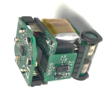
16 An inchworm-inspired motion strategy for robotic swarms

6.2. Swarm Motion Experiments
In the experiments detailed herein, a swarm of millirobots (mROBerTOs) is instructed to follow a
desired (swarm) trajectory – defined by a set of time-phased distinct configurations. Members of the
swarm individually translate and rotate along the given trajectory to achieve the desired
configurations, successively.
 mROBerTO 2.0, developed in our lab at the University of Toronto,12-14 is a millimeter-scale robot
with a swarm sensing module that allows it to accurately measure the relative proximity of nearby
robots through IR communication, Fig. 15 below.
 Front View

 10 mm
Fig. 15. mROBerTO 2.0.

 For swarm localization, inter-robot proximity measurements, obtained by all robots
individually in a decentralized manner, are sent to a host computer through ANT communication.
Here, they are used to estimate the configuration of the swarm through the process detailed in
Section 5. The central computer is also used to select the optimal anchors through the process
detailed in Section 4, and to provide updated motion commands for the mobile robots in each step
of the inchworm motion. The provided motion commands are executed by the robots in an open-
loop and decentralized manner without any intervention from the host computer.
 The specific experiments discussed herein were conducted with a swarm of = 6
mROBerTOs that were instructed to follow a trajectory with = 9 desired configurations. With
performance weights chosen as = 0.5, and = 0.5, the swarm used = 3 anchors to move
between all successive configurations.
 Fig. 16 below illustrates the swarm’s final desired (red), true (blue), and estimated (green)
configurations, once the trajectory is completed. Fig. 17(a)-(b) below are the corresponding plots
of the swarm localization and trajectory following errors versus the swarm’s average total motion
after reaching each successive configuration in the desired trajectory. One may note that the
swarm’s true configuration was measured using an external measurement device. As expected,
motion errors increase as the swarm travels away from its original configuration in open-loop
control. However, as claimed in this paper, the proposed inchworm motion strategy keeps these
errors at very manageable levels.

Fig. 16. Experimental results for swarm localization.

An inchworm-inspired motion strategy for robotic swarms 17

 (a) (b)
Fig. 17. Experimental results: (a) localization error, (b) trajectory-following error.

7. Comparative Analysis
The proposed inchworm sub-strategy is compared, herein, to an alternate anchor-based method
detailed in ref. [57]. The latter divides the swarm into two equal sized subgroups at deployment. The
subgroups remain constant as the swarm follows a trajectory, namely, their number and choice of
member robots do not change.
 The comparative analysis was conducted over a series of simulations. In each, a PTP swarm
trajectory, comprising = 100 desired configurations, was followed. The (cumulative) trajectory-
following performance was calculated as trajectory following error at the very last swarm
configuration (i.e., when the trajectory was completed):
 1
 ∑ 
 =1| − |
 = ̅
 , (24)
 
where and are, respectively, the final true and desired positions of Robot i at . The
trajectory-following performance metric is normalized with respect to the average total motion of all
robots, ̅:
 1 
 ̅ =∑
 ∑
 =1 ( =1 | − ( −1) |) (25)

where is the true position of Robot i once all intermediate steps to have been completed.

 The results of the simulations are detailed in Table I below. In these simulations, the desired swarm
trajectories for a swarm of = 10 robots were generated randomly, changing pose and topology at
each successive desired configuration. In the inchworm experiments, the optimal anchors were
selected through the proposed strategy detailed in Section 4, with = 0.5, and = 0.5. The anchor
robots for the method detailed in ref. [57], however, were selected randomly. Namely, the swarm was
randomly divided into two equal sized subgroups at deployment (i.e., = 5). All simulations were
subjected to random noise in motion command execution and sensing data, as detailed in Section 6
above.
 Table I. Comparative Analysis – Results.
 Trajectory Following Performance, 
 Strategy Sample-Mean Sample-Std-dev
 Ref. [57] 0.0673 0.0500
 Our Method 0.0477 0.0354

 Comparison of the results illustrates that the proposed inchworm sub-strategy is indeed superior
to the method detailed in ref. [57], with a confidence level of at least 97%, Table II below. Both
strategies traversed all desired trajectories with an average of = 5 anchors, illustrating that,
through dynamic anchor selection, the proposed inchworm sub-strategy achieves superior trajectory
following performance without suffering from reduced speed.

18 An inchworm-inspired motion strategy for robotic swarms

 Table II. Comparative Analysis – Confidence Interval.
 Strategy Population-Mean, , 97% Confidence Interval
 Ref. [57] [0.0564 - 0.0782]
 Our Method [0.0400 - 0.0564]

8. Conclusions
This paper presents an inchworm-inspired motion planning strategy developed for achieving accurate
swarm trajectory following. The proposed strategy divides the swarm into two subgroups of anchor
and mobile robots that take turns for incrementally moving towards their destination. Through inter-
robot sensing, the two subgroups cooperate and compensate for their motion uncertainty, thus,
allowing the swarm to achieve enhanced localization and trajectory following performance.
 The proposed inchworm strategy is novel as it dynamically selects the optimal number and choice
of anchor robots as the swarm travels through a series of desired configurations. This flexibility
feature is used to maximize the swarm’s overall motion performance, which consists of two
competing objectives – swarm localization and speed. As a result, the proposed strategy achieves
superior trajectory following performance, when compared to existing methods. Through dynamic
anchor selection, the proposed strategy could also consider other run-time practical constraints, such
as the finite sensing range between swarm robots. In doing so, the motion planning and localization
problems at hand are decoupled. This allows the proposed inchworm motion strategy to work with
any localization method considered.
 A complementary swarm localization method, which fuses inter-robot proximity
measurements and robot motion commands is also presented. This method is novel as it does not
require direct communication between anchor and mobile robots. The proposed localization
method is also applicable to non-anchor based swarm motion strategies, as long as the swarm is
equipped with the necessary sensing technology.
 The inchworm motion strategy was evaluated through a series of physical and simulated
experiments. The physical experiments, conducted with a swarm of mROBerTO millirobots,
illustrated the feasibility of the developed motion planning and localization strategies for real-
world applications, such as human swarm interactions. The performance of the developed
inchworm strategy was also compared to competing methods through extensive trajectory
following simulations. The results illustrate that the proposed strategy achieves significantly
superior trajectory following performance, without suffering from reduced swarm speed.

Acknowledgements
The authors would like to acknowledge the support received, in part, by the Natural Sciences and
Engineering Research Council of Canada (NSERC).

Competing Interests Declaration
Competing interests: The authors declare none.

References
1. E. Şahin, “Swarm Robotics: From Sources of Inspiration to Domains of Application,” In: Swarm
 Robotics (2005) pp. 10–20.
2. M. Brambilla, E. Ferrante, M. Birattari, and M. Dorigo, “Swarm robotics: a review from the swarm
 engineering perspective,” Swarm Intel. 7(1), 1–41 (2013).
3. N. Nedjah and L. S. Junior, “Review of methodologies and tasks in swarm robotics towards
 standardization,” Swarm Evol. Comp. 50, 100565 (2019).
4. M. S. Innocente and P. Grasso, “Self-organising swarms of firefighting drones: Harnessing the power
 of collective intelligence in decentralised multi-robot systems,” J. Comp. Sci. 34, 80–101 (2019).

An inchworm-inspired motion strategy for robotic swarms 19

 5. P. P. Neumann et al., “Indoor Air Quality Monitoring Using Flying Nanobots: Design and
 Experimental Study,” In: IEEE International Symposium on Olfaction and Electronic Nose (2019) pp.
 1-3.
 6. G. A. Cardona and J. M. Calderon, “Robot swarm navigation and victim detection using rendezvous
 consensus in search and rescue operations,” Applied Sciences 9(8), (2019).
 7. C. Eschke, M. K. Heinrich, M. Wahby, and H. Haman, “Self-Organized Adaptive Paths in Multi-Robot
 Manufacturing: Reconfigurable and Pattern-Independent Fibre Deployment,” In: IEEE/RSJ
 International Conference on Intelligent Robots and Systems (2019) pp. 4086–4091.
 8. M. Schranz, M. Umlauft, M. Sende, and W. Elmenreich, “Swarm robotic behaviors and current
 applications,” Front. Robot. AI. 7, (2020).
 9. Z. Kira and M. A. Potter, “Exerting Human Control Over Decentralized Robot Swarms,” In: 4th
 International Conference on Autonomous Robots and Agents (2009) pp. 566–571.
 10. P. Walker, S. A. Amraii, M. Lewis, N. Chakraborty, and K. Sycara, “Human Control of Leader-Based
 Swarms,” In: IEEE International Conference on Systems, Man, and Cybernetics (2013) pp. 2712–
 2717.
 11. S. Shahrokhi, L. Lin, C. Ertel, M. Wan, and A. T. Becker, “Steering a swarm of particles using global
 inputs and swarm statistics,” IEEE Trans. Robot. 34(1), 207–219 (2018).
 12. J. Y. Kim, Z. Kashino, T. Colaco, G. Nejat, and B. Benhabib, “Design and implementation of a
 millirobot for swarm studies – mROBerTO,” Robotica 36(11), 1591–1612 (2018).
 13. J. Y. Kim, T. Colaco, Z. Kashino, G. Nejat, and B. Benhabib, “mROBerTO: A Modular Millirobot for
 Swarm-Behavior Studies,” In: IEEE/RSJ International Conference on Intelligent Robots and Systems
 (2016) pp. 2109–2114.
 14. K. Eshaghi, Y. Li, Z. Kashino, G. Nejat, and B. Benhabib, “mROBerTO 2.0 – An autonomous
 millirobot with enhanced locomotion for swarm robotics,” Robotic. Automat. Let. 5(2), 962–969
 (2020).
 15. W. Ren and R. Beard, “A decentralized scheme for spacecraft formation flying via the virtual structure
 approach,” J. Guide., Control, Dyn. 27, 1746–1751 (2004).
 16. I. Vatamaniuk, G. Panina, A. Saveliev, and A. Ronzhin, “Convex Shape Generation by Robotic
 Swarm,” In: International Conference on Autonomous Robot Systems and Competitions (2016) pp.
 300–304.
 17. M. P. Vicmudo, E. P. Dadios, and R. R. P. Vicerra, “Path Planning of Underwater Swarm Robots Using
 Genetic Algorithm,” In: International Conference on Humanoid, Nanotechnology, Information
 Technology, Communication and Control, Environment and Management (2014) pp. 1-5.
 18. H.-X. Wei, Q. Mao, Y. Guan, and Y.-D. Li, “A centroidal Voronoi tessellation based intelligent control
 algorithm for the self-assembly path planning of swarm robots,” Exp. Syst. App. 85, 261–269 (2017).
 19. Y.-T. Lee, S.-F. Zeng, and C.-S. Chiu, “Distributed Path Planning of Swarm Mobile Robots,” In: 12th
 Asian Control Conference (2019) pp. 49–54.
 20. W. Hönig, J. A. Preiss, T. K. S. Kumar, G. S. Sukhatme, and N. Ayanian, “Trajectory planning for
 quadrotor swarms,” IEEE Trans. Robot. 34(4), 856–869 (2018).
 21. D. Izzo and Pettazzi, “Equilibrium Shaping: Distributed Motion Planning for Satellite Swarm,” In: 8th
 International Symposium on Artificial Intelligence, Robotics and Automation in Space (2005).
 22. V. Gazi, “Swarm aggregations using artificial potentials and sliding-mode control,” IEEE Trans.
 Robot. 21(6), 1208–1214 (2005).
 23. J. R. T. Lawton, R. W. Beard, and B. J. Young, “A decentralized approach to formation maneuvers,”
 IEEE Trans. Robot. Autom. 19(6), 933–941 (2003).
 24. D. Xu, X. Zhang, Z. Zhu, C. Chen, and P. Yang, “Behavior-based formation control of swarm robots,”
 Mathem. Prob. Eng. (2014).

20 An inchworm-inspired motion strategy for robotic swarms

25. C. Bentes and O. Saotome, “Dynamic Swarm Formation with Potential Fields and A* Path Planning
 in 3D Environment,” In: Brazilian Robotics Symposium and Latin American Robotics Symposium
 (2012) pp. 74–78.
26. T. Soleymani and F. Saghafi, “Behavior-Based Acceleration Commanded Formation Flight Control,”
 In: International Conference on Control, Automation and Systems (2010) pp. 1340–1345.
27. L. Consolini, F. Morbidi, D. Prattichizzo, and M. Tosques, “A Geometric Characterization of Leader-
 Follower Formation Control,” In: IEEE International Conference on Robotics and Automation (2007)
 pp. 2397–2402.
28. H. Wang, D. Guo, X. Liang, W. Chen, G. Hu, and K. K. Leang, “Adaptive vision-based leader–follower
 formation control of mobile robots,” Trans. Indust. Electron. 64(4), 2893–2902 (2017).
29. C.-C. Lin, K.-C. Chen, and W.-J. Chuang, “Motion planning using a memetic evolution algorithm for
 swarm robots,” Int. J. Adv. Rob. Syst. 9(1), 19 (2012).
30. K. D. Do and J. Pan, “Nonlinear formation control of unicycle-type mobile robots,” Rob. Auton. Syst.
 55(3), 191–204 (2007).
31. S. M. Ahmadi, H. Kebriaei, and H. Moradi, “Constrained coverage path planning: evolutionary and
 classical approaches,” Robotica 36(6), 904–924 (2018).
32. Y. Chen, S. Ren, Z. Chen, M. Chen, and H. Wu, “Path planning for vehicle-borne system consisting
 of multi air–ground robots,” Robotica 38(3), 493–511 (2020).
33. A. Ashraf, A. Majd, and E. Troubitsyna, “Online path generation and navigation for swarms of UAVs,”
 Sci. Program. 2020, e8530763 (2020).
34. A. Cornejo and R. Nagpal, “Distributed Range-Based Relative Localization of Robot Swarms,” In:
 Selected Contributions of the Eleventh International Workshop on the Algorithmic Foundations of
 Robotics. (2015) pp.107.
35. S. Zhang, E. Staudinger, S. Sand, R. Raulefs, and A. Dammann, “Anchor-Free Localization Using
 Round-Trip Delay Measurements for Martian Swarm Exploration,” In: IEEE/ION Position, Location
 and Navigation Symposium (2014) pp. 1130–1139.
36. M. Berger, L. M. Seversky, and D. S. Brown, “Classifying Swarm Behavior via Compressive Subspace
 Learning,” In: IEEE International Conference on Robotics and Automation (2016) pp. 5328–5335.
37. G. Wagner and H. Choset, “Gaussian Reconstruction of Swarm Behavior from Partial Data,” In: IEEE
 International Conference on Robotics and Automation (2015) pp. 5864–5870.
38. D. S. Brown and M. A. Goodrich, “Limited Bandwidth Recognition of Collective Behaviors in Bio-
 inspired swarms,” In: 13th International Conference on Autonomous Agents and Multiagent Systems
 (2015) pp. 405–412.
39. R. A. Freeman, Peng Yang, and K. M. Lynch, “Distributed Estimation and Control of Swarm Formation
 Statistics,” In: American Control Conference (2006) pp. 7.
40. J. Klingner, N. Ahmed, and N. Correll, “Fault-Tolerant Covariance Intersection for Localizing Robot
 Swarms,” In: Distributed Autonomous Robotic Systems (2019) pp. 485-497.
41. S. Mayya, P. Pierpaoli, G. Nair, and M. Egerstedt, “Localization in densely packed swarms using
 interrobot collisions as a sensing modality,” IEEE Trans. Robotic. 35(1), 21–34 (2019).
42. D. Ma, M. J. Er, B. Wang, and H. B. Lim, “Range-free wireless sensor networks localization based on
 hop-count quantization,” Telecomm. Syst. 50(3), 199–213 (2012).
43. S. Fukui and K. Naruse, “Swarm EKF Localization for a Multiple Robot System with Range-Only
 Measurements,” In: IEEE/SICE International Symposium on System Integration (2013) pp. 796–801.
44. D. Inoue, D. Murai, Y. Ikuta, and H. Yoshida, “Distributed Range-Based Localization for Swarm Robot
 Systems using Sensor-Fusion Technique,” In: 8th International Conference on Sensor Networks (2019)
 pp. 13–22.
45. J. Y. Kim et al., “A high-performance millirobot for swarm-behaviour studies: Swarm-topology
 estimation,” Int. J. Adv. Rob. Syst. 16(6), (2019).