In ation, Oil Price Volatility and Monetary Policy
←
→
Page content transcription
If your browser does not render page correctly, please read the page content below
In‡ation, Oil Price Volatility and Monetary Policy
                   Paul Castilloy           Carlos Montoroz              Vicente Tuestax

                                      First version, October 2005
                                      This version, January 2010

                                                  Abstract

          In a fully micro-founded New Keynesian framework, we characterize analytically the re-
      lation between average in‡ation and oil price volatility by solving the rational expectations
      equilibrium of the model up to second order of accuracy. Higher oil price volatility induces
      higher levels of average in‡ation. We also show that when oil has low substitutability and
      the central bank responds to output ‡uctuations, oil price volatility matters for the level
      of average in‡ation. The model shows that when oil price volatility increases, average in-
      ‡ation increases whereas average output falls: this implies a trade-o¤ also between average
      in‡ation and that of output. The analytical solution further indicates that for a given level
      of oil price volatility, average in‡ation is higher when marginal costs are convex in oil prices,
      the Phillips Curve is convex, and the degree of relative price dispersion is also higher. We
      perform a numerical exercise showing that the model with a empirically plausible Taylor
      rule can replicate the level of average in‡ation observed in the U.S. in 2000s.
          JEL Classi…cation: E52, E42, E12, C63
          Keywords: Oil price volatility, monetary policy, perturbation method, second order
      solution.

      We would like to thank Pierpaolo Benigno, Gianluca Benigno, Juan Dolado, John Dri¢ ll, Jordi Galí, Alberto
Humala, Chris Pissarides, Pau Rabanal, Hajime Tomura, Marco Vega and participants at the research workshop
at the Banco Central de Reserva del Perú, the First Research Workshop on Monetary Policy Asset Prices and Oil
Prices co-organized by the CCBS - Central Bank of Chile and the 12th International Conference on Computing
in Economics and Finance held in Cyprus for useful suggestions and comments. The views expressed herein are
those of the authors and do not necessarily re‡ect those of the Banco Central de Reserva del Perú.
    y
      Banco Central Reserva del Perú.
    z
      Banco Central Reserva del Perú and CENTRUM-Católica. Corresponding author: Carlos Montoro (Email:
carlos.montoro@bcrp.gob.pe), Jr. Miroquesada #441, Lima-Perú. (511)-6132060
    x
      CENTRUM-Católica.

                                                       1
1 Introduction
This paper o¤ers a closed-form solution for the link between in‡ation and oil price volatility:
higher oil price volatility induces higher levels of average in‡ation. This link shifts with several
factors. We show that when oil has low substitutability and monetary policy reacts more
aggressively towards output ‡uctuations, oil price volatility has a larger impact over average
in‡ation. Thus, both monetary policy and the properties of oil have important implications in
the determination of the link between oil price volatility and in‡ation.
Very well known empirical evidence motivates our work. The past forty years were char-
acterized by many periods of oil price shocks with di¤erent implications on both economic
activity and in‡ation. For instance, during the 1970s following the oil price shock (1973 and
1979), in‡ation peaked substantially and GDP declined as well. Nevertheless, in the most
recent period (2002 onwards) the USA economy has experienced an oil price shock of similar
magnitude comparable to that of the 1970s, however, in distinction with the previous episode
both GDP growth and in‡ation have remained relatively stable. Similarly, if we further explore
the link between oil price volatility (measured as the standard deviation of oil price) and both
average in‡ation and output, we attain that larger oil price volatility was associated to high
levels of in‡ation and low levels of output during the 1970s, whereas this link seems to be
broken down in the 2000s. These di¤erent episodes pose questions regarding the link between
oil price volatility and in‡ation: Does oil price volatility matters for the level of in‡ation?, why
the link between oil price volatility and in‡ation has changed recently?, if oil price matters
what would be the role of monetary policy?
Blanchard and Gali (BG, 2008) addressed some of the above questions using a log-linear
New Keynesian model that includes the role of oil as both a production factor and a component
of the consumer price index. BG show that a monetary policy improvement, good luck, more
‡exible labor markets and smaller share of oil in production have had an important role in
explaining the di¤erent macroeconomic performance between the 1970s and 2000s. The log-
linear approximation, however, might o¤er an inaccurate solution when shocks are relatively
large, substantially increasing the approximation error of the model´s solution. Indeed, as the
empirical evidence corroborates, oil price shocks are hefty compared to other shocks usually
appended in traditional new-Keynesian models (like monetary and productivity shocks). More
importantly, the log-linear solution misses crucial channels through which oil price a¤ect in‡a-
tion, such as its own volatility, the precautionary behavior of price setters and the convexity of
the Phillips Curve. In a nutshell, a log-linear solution is incapable to tell us something about
a link between oil price volatility and average in‡ation.
Thus, in this paper we complement BG work and deal with the aforementioned limitations
2arising from log-linear approximations by providing a tractable and uni…ed framework to ana-
lyze the e¤ects of oil price volatility on in‡ation. Our framework allows us to shed additional
light beyond those o¤ered by log-linear solutions on the nature of the apparent changes in the
macroeconomic e¤ects of oil prices. In essence, we establish the link between oil price volatility
and average in‡ation. In doing so, we use a standard New Keynesian micro-founded model
with staggered Calvo pricing where the central bank implements its policy following a Taylor
rule. We modify this simple framework considering oil as a production input for intermediate
good that is di¢ cult to substitute in production. Then, we solve up to second order of accuracy
the rational expectations equilibrium of this model using the perturbation method developed
by Schmitt-Grohé and Uribe (2004).
The second order solution has the advantage of incorporating the e¤ects of shocks volatility
in the equilibrium, which are absent in the linear solution. We implement this method both
analytically and numerically. As part of our contribution, we use an original strategy to obtain
an analytical solution. Thus, di¤erent from other papers in the literature such as Aruoba et.
al. (2006) and Schmitt-Grohé and Uribe (2005), in which the perturbation method is applied
directly to the non-linear system of equations, we …rst approximate the model up to second
order and then apply the perturbation method to the approximated model. This strategy
permits us to disentangle the key determinants of the relationship between oil price volatility
and in‡ation and to quantify the importance of each determinant in general equilibrium.
Our basic …nding indicates that the second order analytical solution - by relaxing certainty
equivalence- permits us establishing a link between oil price volatility and average in‡ation.
Just to highlight some parallelism, this level of in‡ation generated by oil price volatility is
similar to the e¤ect of consumption volatility on the level of average savings studied in the
literature of precautionary savings. Indeed, the solution up to second order shows that oil price
volatility produces an extra level of in‡ation by altering the way in which forward-looking …rms
set their prices. This mechanism is absent in log-linear solutions and the link arises from the
forward-looking behavior of the optimizing agents.
On the sources of the link between oil price volatility and in‡ation, the analytical solution
shows the following: …rst, when oil has low substitutability, marginal costs are convex in
oil price, hence, its price volatility raises the expected value of marginal costs. Second, oil
price volatility in itself generates in‡ation volatility, thus inducing price setters to be more
cautious to future expected marginal costs. In particular, producer relative prices become more
sensitive to marginal costs, amplifying the previous channel. Third, relative price dispersion,
by increasing the amount of labor required to produce a given level of output, increases average
wages, thus amplifying the e¤ect of expected marginal costs over average in‡ation. Fourth,
in general equilibrium, the weights that the central bank assigns on in‡ation and output
3are key determinants for the level of in‡ation induced by oil price volatility. As a result, our
model predicts that the smaller (larger) the endogenous responses of a central bank to in‡ation
(output) ‡uctuations, the greater the average in‡ation (smaller average output). Thus, changes
in the way monetary policy was conducted may explain di¤erent responses of the economy to
oil price volatility and oil shocks. This …nding is consistent with the fact that, in the model,
oil price generates a monetary policy trade-o¤ between stabilizing in‡ation and output, which
traduces to a policy trade-o¤ in means as well.
We also evaluate the implications of analytical results of the model by performing a …rst
pass numerical exercise calibrated for the U.S. economy. Overall, our results are broadly
consistent with predictions of the analytical solution. In addition, we are able to generate
a level of average in‡ation similar to the one observed during the 2000s. We show that the
commitment of U.S. central bank to maintain low and stable levels of in‡ation, helped to
improve the trade-o¤ between in‡ation and output in 2000s, despite oil price volatility was of
similar magnitude to that observed in the 1970s. We further …nd others factors important in
explaining the link between in‡ation and oil price volatility in the 2000s. For example, the
convexities of the Phillips curve and price dispersion explain 44 and 38 percent, respectively,
of the level of average in‡ation in the 2000s. Last but not least, we devote a section to analyze
the accuracy of the second order approximation showing the gains of it, relative to the linear
solution, in terms of errors of the in‡ation´s equation.
Other authors introduced the second order approach in closed and open economies; however,
most of the studies have mainly focused on welfare evaluations across di¤erent environments.
For example Benigno and Woodford (2003) implemented the second order solution to evaluate
optimal monetary and …scal policy in a closed economy. Benigno and Benigno (2005) used
the second order approach to evaluate the optimal policy in a two-country model with com-
plete markets. Two studies could be seen, methodologically, closer to our work. Evans and
Hnatkovska (2005) evaluated the role of uncertainty in explaining di¤erences in the holding of
assets in two-country models and Obstfeld and Rogo¤ (1998) developed an explicit stochastic
NOEM model relaxing the assumption of certainty equivalence. The latter authors, based on
simpli…ed assumptions, obtained an analytical solution for the level exchange rate premium.
Di¤erent from the aforementioned two studies, in this paper we obtain an analytical solu-
tion for the extra level of in‡ation arising from the second order approximation using a fully
micro-founded New Keynesian model with oil prices.
The rest of the paper is organized as follows. Section 2 presents some basic facts for the
US economy to motivate on the link between oil price volatility and in‡ation. In also provides
a simple model that supports the link. Section 3 presents the model. Section 4 explains the
mechanism at work in generating the link between oil prices and in‡ation. Section 5 uses the
4model to analyze the role of oil price volatility and monetary policy for the level of average
in‡ation and perform some numerical exercises. Section 6, for robustness, analyzes the degree
of accuracy of the second order solution. Finally section 7 concludes.
2 Motivation
2.1 Average in‡ation and oil price volatility
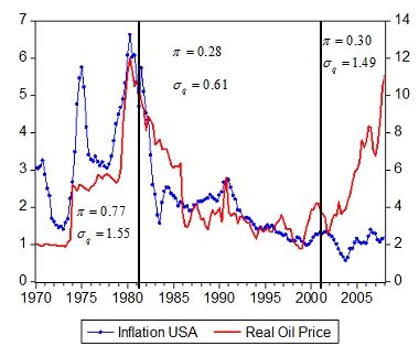
Inspection of US in‡ation and oil price data seems to suggest that both in‡ation rate and oil
prices have moved together from 1970 until 1999. However, from 2000 onwards this positive co-
movement has broken down. Figure 1 displays the evolution of the real price of oil and in‡ation
both in logs since 1970. We measure oil price as the log spot price West Texas Intermediate
minus log SA non-farm business sector de‡ator and our measure of in‡ation is the variation
of the consumer price index. The …gure shows that, from 1970 until the beginning of 2000s,
the dynamics of in‡ation evolves closely to that of oil price. Thus, for the period 1970-1980
we observe a persistent initial increase in in‡ation vis-à-vis a jump in oil price following the oil
price shock in 1974. From 1980 to 1999 we observe a steady decline in in‡ation accompanied
by a persistent drop in oil price. Unlike the …rst two sub-samples, from 2002 onwards the
Figure shows a markedly upward trend in oil price and a moderate increase in in‡ation. It
seems that the positive relationship between in‡ation and oil price became weaker during the
more recent period.
This di¤erent dynamics witnessed during the 2002s is also evident when comparing the
standard deviation of oil price with average in‡ation across the same sub-samples1 .Table 1
reports the standard deviations and averages levels of both oil price and in‡ation for the
three sub-samples, 1970-1983, 1984-2002 and 2002-2008. Again, by comparing the …rst and
second sub-samples, note that a high level of average in‡ation and high volatility of oil price
characterizes the …rst one, whereas a lower level of both average in‡ation and volatility of
oil price typi…es the second one. This very simple evidence indicates a positive relationship
between oil price volatility and average in‡ation during the two …rst sub-samples. Nevertheless,
in the 2000s this relation has changed dramatically. From 2002-2008, oil price volatility is as
large as the one reported in the …rst sub-sample (1.49 in 2000s versus 1.55 in 1970s), however,
the average level of in‡ation is three times smaller. The description of these stylized facts is
not altered if we use other measures of in‡ation and oil price.
1
BG identify four shocks using as a de…nition of oil shock as an episode involving a cumulative change in the
(log) price of oil above 50 percent, sustained for more than four quarters. Our two …rst sub-samples contain the
three …rst identi…ed shocks and the last sub-sample contains the fourth shock reported in BG.
5Figure 2.1: U.S. In‡ation and Real Oil Price
Table 1: In‡ation and Real Oil Price
(I) 1970-1983 (II) 1984-2002 (III) 2002-2008
S.D. In‡ation 0.77 0.28 0.30
S.D. Real Oil Price 1.55 0.61 1.49
Mean In‡ation 1.57 0.53 0.57
Mean Real Oil Price (1970=1) 2.87 2.17 4.30
We summarize the evidence reported above as follows: First, there is a positive link between
oil price volatility and average in‡ation rate during the …rst two sub-samples. Second, this
positive link has broken down from 2002 onwards. The above two pieces of evidence are the
main motivation of our paper. In the next sections, …rst we develop a new Keynesian model
that permits us to obtain, analytically, a positive link between oil price volatility and average
in‡ation. Second, with the model and the link at hand, we explore the reasons why this link
might have been broken down or has been less important during the 2000s.
2.2 The link in a simple model
Before moving to a general equilibrium analysis, in this section we use a simple model to
establish a link between average in‡ation and oil price volatility. Suppose that …rms produc-
ing di¤erentiated goods set prices one period in advance. They also face a downward sloping
6Pt (z) "
demand function of the type, Yt (z) = Pt Y; where " represents the elasticity of sub-
stitution across goods and Y aggregate output, which is …xed. Under these assumptions, the
optimal pricing decision of a particular …rm z for time t is given by a mark-up over the expected
next period marginal cost,
Pt (z)
= Et 1[ t M Ct ] (2.1)
Pt 1
"+1
where , M Ct and t = t
Et 1 "t denote the mark-up, …rm´s marginal costs and a measure of
the responsiveness of the optimal price to future marginal costs, respectively. The previous
arguments are standard in new Keynesian frameworks. A second order Taylor expansion of
the expected responsiveness to marginal cost, t; is given by:
1 2
Et 1[ t] = Et 1 t + (2" + 1) t (2.2)
2
From the above expression it is clear that Et 1 t is a convex function of expected in‡ation.
This convexity implies that in‡ation volatility increases the weight that a …rm assigns on
expected marginal costs. Thus, for the same level of marginal costs, an increase in in‡ation
volatility generates a rise in in‡ation.
To gain further insights, let us assume the following quadratic marginal cost function in
terms of oil prices (the only input for production is oil)
2 2
M Ct = 1 qt + qt (2.3)
2
where qt denotes the real price of oil, 1 > 0 measures the linear e¤ect of oil over the marginal
cost and 2 accounts for the impact of oil price volatility on marginal costs. When 2 > 0,
marginal costs are convex in oil prices, hence expected marginal costs become an increasing
function of oil price volatility.2
Di¤erent forms of aggregation of sticky prices in the literature show that the in‡ation rate is
proportional to the optimal relative price of …rms (equation (2.1)). Thus, when marginal costs
are convex, both the optimal relative price and in‡ation are increasing in oil price volatility.
More importantly, other channels amplify the previous e¤ect. To the extent that oil price
volatility induces an increase in in‡ation volatility, price setters react by augmenting the weight
on marginal costs, t, when setting their prices. As equation (2.2) indicates, up to second order,
the weight, t; depends not only on the level of expected in‡ation but also on its volatility.
Nevertheless, it is fair to raise the question whether or not those second order e¤ects are
2
In section 4 we show that when the production function is a CES with an elasticity of substitution between
labor and oil lower than one, marginal costs are convex in oil prices, that is 2 > 0.
7important. As it will become clearer later in the paper, two special features of oil prices are
crucial to make those second order e¤ects quantitative sizable: a) its high volatility and b) its
low substitutability with other production factors.
A linear approximation that omits the role of both oil price and in‡ation volatilities would
not capture the e¤ects of oil price volatility over average in‡ation. In contrast, the second order
solution of the rational expectations equilibrium of the model allows us to include volatility
terms as determinants of the level of average in‡ation.
So far we showed that a second order solution allows us to establish a positive link between
the volatility of oil prices and the average level of in‡ation. Indeed, this positive relationship
can potentially explain the empirical evidence during the 1970s, that is, the higher the volatility
of oil price the higher the average level of in‡ation.
Note also that in a micro-founded new Keynesian framework, 1 and 2 represent reduced
form parameters. For example, in such an environment, 2 measures the sensitivity of the
average level of in‡ation to oil price volatility, and it will depend on deep parameters, among
them, those associated with the conduct of monetary policy (reaction function). Thus as an
example, if 2 falls due to a change in the central bank reaction function (i.e. more aggressive
towards in‡ation), the e¤ect of oil price volatility, qt2 , can be dampened and even completely
o¤set. This is consistent with the hypothesis that monetary policy has been more aggressive
in the late 1990s than in the 1970s. In the next section we formalize this link by deriving
a second order rational expectations solution of a New Keynesian general equilibrium model
with oil prices.
3 A new Keynesian model with oil prices
The model economy corresponds to the standard New Keynesian model. We follow Blanchard
and Gali (2008) in introducing a non-produced input M , represented in this case by oil. Q
denotes the real price of oil which is exogenous.
3.1 Households
We assume the following utility function on consumption and labour of the representative
consumer
1
X
t to Ct1 L1+v
t
Uto = Eto ; (3.1)
t=to
1 1+v
where and represent the coe¢ cient of risk aversion and the inverse of the elasticity of labor
supply, respectively. The optimizer consumer takes decisions subject to a standard budget
8constraint which is given by
Wt Lt Bt 1 1 Bt t Tt
Ct = + + + ; (3.2)
Pt Pt R t Pt Pt Pt
where Wt is the nominal wage, Pt is the price of the consumption good, Bt is the end of
period nominal bond holdings, Rt is the nominal gross interest rate , t is the share of the
representative household on total nominal pro…ts, and Tt are transfers from the government.3
The …rst order conditions for the optimizing consumer´s problem are:
" #
Pt Ct+1
1 = E t Rt ; (3.3)
Pt+1 Ct
Wt
= Ct Lt = M RSt : (3.4)
Pt
Equation (3:3) is the standard Euler equation that determines the optimal path of consump-
tion. At the optimum the representative consumer is indi¤erent between consuming today or
tomorrow, whereas equation (3:4) describes the optimal labor supply decision. M RSt denotes
the marginal rate of substitution between labor and consumption. We assume that labor mar-
kets are competitive and also that individuals work in each sector z 2 [0; 1]. Therefore, L
corresponds to the aggregate labor supply:
Z 1
L= Lt (z)dz: (3.5)
0
3.2 Firms
3.2.1 Final goods producers
There is a continuum of …nal goods producers of mass one, indexed by f 2 [0; 1] that operate
in an environment of perfect competition. They use intermediate goods as inputs, indexed by
z 2 [0; 1] to produce …nal consumption goods using the following technology:
Z 1
"
" 1
" 1
Ytf = Yt (z) " dz ; (3.6)
0
where " is the elasticity of substitution between intermediate goods. Then the demand function
of each type of di¤erentiated good, is obtained by aggregating the input demand of …nal good
3
The government owns the oil´ s endowment which is produced in the economy at zero cost and sold to the
…rms at an exogenous price. The government transfers all the revenues generated by oil to consumers, that is:
Tt
Pt
= Qt Mt .
9producers
"
Pt (z)
Yt (z) = Yt ; (3.7)
Pt
where the price level is equal to the marginal cost of the …nal good producers and is given by:
Z 1
1
1 "
1 "
Pt = Pt (z) dz ; (3.8)
0
and Yt represents the aggregate level of output.
Z 1
Yt = Ytf df: (3.9)
0
3.2.2 Intermediate goods producers
There is a continuum of intermediate good producers indexed by z 2 [0; 1]. All of them have
the following CES production function
h 1 1 i 1
Yt (z) = (1 ) (Lt (z)) + (Mt (z)) ; (3.10)
where M is oil which enters as a non-produced input; represents the intratemporal elasticity
of substitution between labor-input and oil and denotes the share of oil in the production
function. We use this generic production function to account for the fact that oil has few
substitutes ( < 1). Since oil has few substitutes an appealing functional form to capture this
feature is the CES production function. This function o¤ers ‡exibility in the calibration of
the degree of substitution between oil and labor.4 The oil price shock, Qt , follows an AR(1)
process in logs,
log Qt = (1 ) log Q + log Qt 1 + "t ; (3.11)
where Q is the steady state level of oil price. From the cost minimization problem of the …rm
we obtain an expression for the real marginal cost given by:
" # 1
1 1
Wt
M Ct (z) = (1 ) + (Qt )1 ; (3.12)
Pt
4
Some authors that have included oil in the analysis of RBC models and monetary policy, have omitted
this feature. For example, Kim and Loungani (1992) assume for the U.S. a Cobb-Douglas production function
between labor and a composite of capital and energy. Given that they calibrate their model considering that
oil has a small share on output, they found that the impact of oil in the U.S. business cycle is small. Notice
that when = 1; the production function collapses to the standard Cobb-Douglas function as the one used by
Blanchard and Gali (2006): Yt (z) = (Lt (z))1 (Mt (z)) :
10where M Ct (z) ; Wt and Pt represents the real marginal cost, nominal wages and the consumer
price index, respectively. Note that since technology has constant returns to scale and factor
markets are competitive, marginal costs are the same for all intermediate …rms, i.e. M Ct (z) =
M Ct . The individual …rm´s labor demand is given by:
1 Wt =Pt
Ldt (z) = Yt (z): (3.13)
1 M Ct
Intermediate producers set prices following a staggered pricing mechanism a la Calvo. Each
…rm faces an exogenous probability of changing prices given by (1 ). The optimal price that
solves the …rm’s problem is given by
P
1
k "+1
Et t;t+k M Ct+k Ft;t+k Yt+k
Pt (z) k=0
= ; (3.14)
Pt P
1
k "
Et t;t+k Ft;t+k Yt+k
k=0
" k Ct+k Pt
where " 1 is the price markup, t;t+k = Ct Pt+k is the stochastic discount factor,
P
Pt (z) is the optimal price level chosen by the …rm, Ft;t+k = Pt+k
t
denotes the cumulative level
of in‡ation and Yt+k is the aggregate level of output. Since only a fraction (1 ) of …rms
changes prices every period and the remaining share keeps its price …xed, thus the aggregate
price level -the price of the …nal good that minimize the cost of the …nal goods producers- is
given by the following equation:
Pt1 "
= Pt1 1
"
+ (1 ) (Pt (z))1 "
: (3.15)
Following Benigno and Woodford (2005), equations (3:14) and (3.15) can be written recursively
introducing the auxiliary variables Nt and Dt (see appendix B:1 for details):
1 "
" 1 Nt
( t) =1 (1 ) ; (3.16)
Dt
h i
" 1
Dt = Yt (Ct ) + Et ( t+1 ) Dt+1 ; (3.17)
"
Nt = Yt (Ct ) M Ct + Et [( t+1 ) Nt+1 ] : (3.18)
Equation (3:16) comes from the aggregation of individual …rms prices. The ratio Nt =Dt repre-
sents the optimal relative price Pt (z) =Pt : Equations (3.16), (3.17) and (3.18) summarize the
recursive representation of the non- linear Phillips curve. Writing the optimal price setting
11in a recursive way is necessary in order to implement both numerically and algebraically the
perturbation method.
3.3 Monetary policy
The central bank conducts monetary policy by targeting the nominal interest rate according
to the following Taylor-type rule
" #1 r
r
Et t+1 Yt y
Rt = Rt 1 R ; (3.19)
Y
where, > 1 and y > 0 measure the response of the nominal interest rate to expected future
in‡ation and current output, respectively. The degree of interest rate smoothing is measured
by 0 r 1: The steady state values are expressed without time subscript and with and
upper bar.
3.4 Market clearing
Labor, intermediate and …nal goods markets clear. Since there is neither capital accumulation
nor government sector, the economy-wide resource constraint is given by
Yt = Ct : (3.20)
The labor market clearing condition is given by:
Lt = Ldt : (3.21)
Where the demand for labor comes from the aggregation of individual intermediate producers
in the same way as the labor supply:
Z 1 Z 1
1 Wt =Pt
Ld = Ldt (z)dz = Yt (z)dz; (3.22)
0 1 M Ct 0
1 Wt =Pt
Ld = Yt t;
1 M Ct
R1 Pt (z)
"
where t = 0 Pt dz is a measure of price dispersion. Since relative prices di¤er across
…rms due to staggered price setting, input usage will di¤er as well. Thus, it is not possible to use
the usual representative …rm assumption. Therefore, the price dispersion factor, t; appears
in the aggregate labor demand equation. From (3.22) note that higher the price dispersion the
12larger the labor amount necessary to produce a given level of output.
4 The second order representation
4.1 The second-order Taylor expansion
As previously mentioned, the special features of oil, such as its high price volatility and its low
substitutability in production, imply that oil prices can have meaningful second-order e¤ects on
in‡ation in addition to those usually shown to be important in log-linear models. In log-linear
representations certainty equivalence holds, thus uncertainty does not play any role. Thus,
to gauge the link between oil prices and in‡ation, a second-order solution is required. To
characterize this solution, we present a log-quadratic Taylor approximation of equations (3.3),
(3.4),(3.12), (3.16), (3.17), (3.18), (3.19 ) and (3.22) around the deterministic steady-state.5
The second-order Taylor-series expansion serves to compute the equilibrium ‡uctuations of
2
the endogenous variables of the model up to a residual of order O kqt ; qk where q is the
standard deviation of the real oil price and kqt ; q k denotes a bound on both the deviation
of oil price from its steady state and its 6
volatility. We denote variables in steady state with
upper bar (i.e. X) and their log deviations around the steady state with lower case letters
(i.e. x = log( X
X )). After imposing the goods and labor market clearing conditions to eliminate
t
real wages and labor from the system, the dynamics of the economy is given by the following
equations:
5
Appendix B:2 provides a detailed derivation of the log-quadratic Taylor approximations. See appendix A
for the derivation of the steady-state of the economy.
6
Since we want to make explicit the e¤ects of changes in oil price volatility over the equilibrium of the
endogenous variables, we solve the policy functions as in Schmitt-Grohe and Uribe (2004) in terms of the shocks
(qt ) and its volatility, ( q ). This approach is di¤erent to the one undertook by Benigno and Woodford (2003),
for example, who considers a policy function in terms of the shocks only (et ).
13Table 2: Second order Taylor expansion of the equations of the model
Marginal Costs
mct = ( + ) yt + (1 ) qt + 12 (1 ) 2 11 (( + ) yt qt )2 + v b t + O kqt ; qk
3
(i)
where the price dispersion is de…ned by:
bt = bt 1 + 1" 2
t + O kqt ; q k
3
(ii)
2 1
Phillips Curve
1
t = mct + 2 mct (2 (1 ) yt + mct ) + 12 " 2t + Et t+1 + O kqt ; q k3 (iii)
where we have de…ned the auxiliary variables:
1 " 1 2 1
t t + 2 1
+" t + 2
(1 ) t zt (iv)
2" 1 2
zt 2 (1 ) yt + mct + Et 1 t+1 + zt+1 + O kqt ; qk (v)
Aggregate Demand
2 3
yt = Et yt+1 1 (rt Et t+1 ) 12 Et (yt yt+1 ) 1
(rt t+1 ) + kqt ; qk (vi)
Policy Rule
rt = r rt 1 + (1 r) Et t+1 + y yt (vii)
Oil process
qt = qt 1 + q et (viii)
1
1 Q 1
where 1+v , MC
, (1 ), and Q, and M C denote the
steady-state value of oil price and marginal costs, respectively. The …rst …ve equations of table
2 summarize the second-order expansion of the aggregate supply curve, whereas the sixth
equation is the second-order expansion of the aggregate demand. We obtained equation (i) by
taking a second-order Taylor-series expansion to the real marginal cost equation after replacing
real wages with its equilibrium determinants. The term b t , equation (ii), is the log-deviation
of the measure of price dispersion t, which is a second order function of in‡ation. Overall,
these equations indicate that in an economy with volatile oil prices, not only expected marginal
costs, expected oil price, and expected future in‡ation matter for in‡ation dynamics but also
their second moments. For instance, the second order approximation adds two new ingredients
to the determination of the marginal cost. The …rst one is related to the convexity of marginal
costs with respect to oil price. From equation (i) note that, when oil is di¢ cult to substitute,
< 1, the marginal cost becomes a convex function of oil price, hence, oil price volatility
induces an increase in the expected marginal cost. This is an important channel through
which oil price generates higher in‡ation rates absent when using Cobb-Douglas production
function : When = 1; the marginal cost equation boils down to
mct = ( + ) yt + (1 ) qt + v b t
Note that, in the above equation, the marginal cost does not depend directly on the volatility
of oil prices q 2 , but only indirectly through its e¤ects on relative price dispersion term, b t .
t
14The second new ingredient in equation (i) is the price dispersion term b t . It is clear that
as price dispersion increases, the required number of hours to produce a given level of output
also increases. The higher labor demand further increases real wages and therefore marginal
1
cost also increase. This e¤ect is higher the lower the elasticity of labor supply, v; and the
higher the share of oil in production.
The second order representation of the aggregate demand considers also the e¤ect of growth
rate of consumption volatility on savings. Thus, when the volatility of consumption increases,
consumption falls, since households increase their savings for precautionary reasons.
4.2 The canonical representation
Next we further simplify the model by plugging equations (i),(ii),(iv) and (v) in equation (iii),
and the policy rule of the central bank (vii) in equation (vi). To make the analysis analytically
tractable, we set the smoothing parameter in the Taylor rule equal to zero. Similarly, we
assume an small initial price dispersion such that b to 1 0 up to second order.7 Thus,
the model collapses to a second- order system of two-equations as a function of in‡ation and
output: an aggregate supply equation (4.1) and an aggregate demand equation (4.2) )
1 2 1 3
t = y yt + q qt + Et t+1 + ! q + ( mc + + ) qt2 + O kqt ; qk (4.1)
2 2
1 1 2 3
yt = Et (yt+1 ) ( 1) Et t+1 + y yt + !y q + O kqt ; qk (4.2)
2
where y ( + ) , and q (1 ) . To get the above two equations, we write the
second-order terms of the endogenous variables as functions of 2 and qt2 , using the …rst-order
q
solution of the model as in Sutherland (2002). As equation (4.1) shows, both the conditional
and unconditional variances of oil price are relevant for the determination of average in‡ation.
The magnitude of the impact of these second moments on average in‡ation depends on the
following “omegas” coe¢ cients: mc measures the impact of qt2 on marginal costs, , on 2
t ,
on , similarly, ! and ! y measure the impact of 2 on in‡ation and output, respectively.
t q
Those coe¢ cients are derived in appendix B. Note that if the aforementioned coe¢ cients were
equal to zero the model would collapse to a standard version of a New Keynesian model
in log linear form. In the next section, we obtain the link between in‡ation and oil price
volatility by solving the rational expectations equilibrium for f t g and fyt g using (4.1) and
(4.2). Yet, before moving to the analytical solution we perform some simulations showing how
7
This notwithstanding, the numerical exercises consider the more general speci…cation of the model and
qualitatively results are broadly the same.
15the “omegas” coe¢ cients depend upon deep parameters. To perform the simulation we use
the benchmark parameterization of section 5.3.
mc coe¢ cient measures both the direct e¤ect of oil price volatility on marginal costs and
its indirect e¤ect through the labor market. Let’s …rst consider the direct e¤ect. When oil has
few substitutes, < 1, the …rm´s marginal cost is convex in oil prices, hence, the expected
marginal cost becomes an increasing function of oil price volatility. To compensate any increase
in expected marginal costs triggered by oil price volatility, a forward looking …rm reacts by
optimally charging a higher price. In turn, this …rm´s response leads to higher aggregate
in‡ation when prices are sticky.8 Interestingly, the smaller the elasticity of substitution between
oil and labor inputs, the larger the increase in both marginal costs and in‡ation in response
to oil price volatility. Oil price volatility further a¤ects the marginal cost indirectly, through
its e¤ects on the labor market. Since oil price volatility generates in‡ation volatility, which
is costly because it increases relative price distortions, e¢ ciency in production falls as the
volatility of oil prices rises. In particular, …rms require, at the aggregate level, more hours of
work to produce the same amount of output. Hence, the demand for labor rises, making labor
more expensive and consequently the marginal cost and in‡ation augment even further.
Panels (a) and (b) in …gure 4.1 depict the relation between mc and the elasticity of substi-
tution between oil and labor inputs, ; and the steady state level of oil prices, Q; respectively.
As shown in panel (a), the lower the elasticity of substitution, ; the higher the direct e¤ect
of oil price volatility over marginal costs. Moreover, the higher the steady state level of oil
price, ceteris paribus, the higher the e¤ect of oil price volatility on marginal costs. Overall
these simulations suggest that economies where oil has less substitutes or oil price is large, oil
price volatility in itself would have a larger impact on average in‡ation.
Coe¢ cient accounts for the e¤ects of oil price volatility on the weight …rms assign
to movements in future marginal costs. When prices are sticky and …rms face a positive
probability of not being able to change prices, as in the Calvo price-setting model, the weight
that …rms assign to future marginal cost depends on both expected in‡ation and in‡ation’s
volatility. Thus, oil price volatility by raising in‡ation volatility induces price-setters to put
a higher weight on future marginal costs. In a nutshell, oil price volatility not only increases
expected marginal costs but also it makes the …rms´ relative prices to be more sensitive to
future marginal costs. In fact, panel (c) in …gure 2 shows that the lower the degree of price
stickiness, ; the larger the e¤ect of oil price volatility over in‡ation volatility, . The previous
8 @ 2 mct 21
This mechanism can be understood by observing equation (i), where @qt2
= (1 ) 1
. When <
2
@ mct
1( > 1), @qt2
> 0(< 0)
16Figure 4.1: Average in‡ation components.
17relation comes from the fact that lower price rigidity makes the Phillips curve steeper and more
convex, making the e¤ect of in‡ation volatility larger. Panel (d) shows that when the elasticity
of substitution of goods, "; increases, the e¤ect of in‡ation volatility on the individual price of
…rms, ; increases.
Coe¢ cients and ! account for the time variant and constant e¤ects of in‡ation volatil-
ity on the composite of in‡ation t, respectively. Both mechanisms are similar to the ones
associated to , however, both coe¢ cients are quantitatively small. Finally, the coe¢ cient
! y is negative and accounts for the standard precautionary savings e¤ect, by which oil price
volatility induces households to increase their savings to bu¤er future states of the nature when
income is low.
5 Oil price volatility and in‡ation in general equilibrium
5.1 The equilibrium level of average in‡ation
We use the perturbation method to obtain the second order rational expectations solution of
the model.9 Di¤erent from other papers which apply perturbation methods directly to the
non-linear system of equations, we …rst approximate the model up to second order and then
implement the perturbation method.10 Our approach has the advantage that makes it easier to
obtain clear analytical results for the link between the level of in‡ation and oil price volatility.
We write the rational expectations second order solution of output and in‡ation, in log-
deviations from the steady state, as quadratic polynomials in both the level and the standard
deviation of oil price shock:
1 1
yt = ao 2
q + a1 qt + a2 (qt )2 + O kqt ; q k3 (5.1)
2 2
1 2 1 2 3
t = bo q + b1 qt + b2 (qt ) + O kqt ; q k (5.2)
2 2
3
where the as and bs are the unknown coe¢ cients that we need to solve for and O kqt ; qk
9
We implement the perturbation proposed by Schmitt-Grohe and Uribe (2004). This method was originally
developed by Judd (1998) and Collard and Julliard (2001). The …xed point algorithm proposed by Collard and
Julliard introduces a dependence of the coe¢ cients of the linear and quadratic terms of the solution with the
volatility of the shocks. In contrast, the advantage of the algorithm proposed by Schmitt-Grohe and Uribe is
that the coe¢ cients of the policy are invariant to the volatility of the shocks and the corresponding ones to the
linear part of the solution are the same as those obtained solving a log linear approximated model, which makes
both techniques comparable.
10
Since a second order Taylor expansion is an exact approximation up to second order of any non-linear
equation, having the system expressed in this way will give us the same solution as the system in its non-linear
form.
18denotes terms on q and q of order equal or higher than three.11 Notice that the linear terms
a1 qt and b1 qt correspond to the policy functions that we would obtain using any standard
method for linear models (i.e. undetermined coe¢ cients), whereas the additional elements
ao ; b0 ; a2 and b2 ; account for the e¤ects of second moments. The quadratic terms in the policy
1 2 1 2
function of in‡ation have two components: 2 bo q , which is constant and 2 b2 (qt ) ; which is
time varying. Taking the unconditional expectation to equation (5:1) we obtain the level of
average in‡ation as a function of oil price shock volatility and deep parameters
1 2
E( )= (bo + b2 ) q
2
The perturbation method helps us to recover parameters bo and b2 ; thus allowing us to get an
expression for the level of average in‡ation which reads as follows:
1 1 2
E( )= y ( mc + + ) (1 + ) + y! + y !y q (5.3)
2 0
where 0 ( 1) y + (1 ) y > 0: Equation (5.3) indicates that not only the …rst
moments of oil price a¤ect in‡ation but also its volatility. According to the above equation, the
link between average in‡ation and oil price volatility depends crucially on how monetary policy
is conducted and on the “omegas” coe¢ cients, where the latter are linked to the convexity of
both marginal costs and the Phillips curve. In Appendix B.4 we show that the parameter
is positive. Thus, if 0 > 0; average in‡ation is always positive, when it holds that
y > !y y = [! +( mc + + ) (1 + )] > 0 (5.4)
since ! y is negative, the right hand side is positive. In this case, average in‡ation is increasing
on the “omegas” coe¢ cients.
5.2 The role of monetary policy
The way the central bank implements its monetary policy plays a crucial role on the positive
link between oil price volatility and average in‡ation. First, a necessary condition for this link
to exist is that the central bank rises interest rates in response to output ‡uctuations, y > 0.
This is so because in this case, a sharp increase in oil prices does not lead the central bank to
raise interest rates by so much, implicitly allowing the oil price shock to generate higher and
more volatile in‡ation levels, which, as we described before, generates higher average in‡ation.
Yet, if the central bank cares only about in‡ation and does not react to output ‡uctuations,
11
Schmitt-Grohe and Uribe (2004) show that the quadratic solution does not depend neither on q nor on
qt q . That is, they show that the coe¢ cients in the solution for those terms are zero.
19that is y = 0, the model predicts that average in‡ation would be negative and small even if
oil prices are very volatile. In this case, the oil price shock generates a sharp fall in output
triggered by the precautionary savings behavior of households, which more than compensate
the impact of oil prices on in‡ation through a fall in labor costs. This restriction, however is
weaken when households do not exhibit precautionary savings, ! y = 0: In this case, the link
between oil price volatility and average in‡ation is positive even when, y = 0: Moreover, as
it is shown in Montoro (2010), in this setup it is optimal for the central bank to react both
to in‡ation and output ‡uctuations, since oil prices generate an endogenous trade-o¤ between
stabilizing in‡ation and the e¢ cient output gap. This endogenous trade o¤ emerges from the
combination of a distorted steady state and a CES production function.12
Second, there exist an interesting association between the size of average in‡ation and the
well known Taylor principle. Note that the denominator of expression (5:3) ; 0; is not other
thing that the condition that guarantees uniqueness of the rational expectations equilibrium
in the canonical new Keynesian model, known as the Taylor principle. To the extent that
y > 0 and above the small threshold needed for having positive average in‡ation, the larger
the reaction to in‡ation, ; the larger 0; and consequently the smaller the level of average
in‡ation. While the degree of average in‡ation is larger when y is larger, this relation weakens
when the central bank reacts more aggressively to in‡ation (larger ). Note also that for small
values of there are meaningful di¤erences in the levels of average in‡ation when changing
the reaction to output ‡uctuations.
A fundamental implication of this analysis is that monetary policy can mitigate the e¤ects
of oil price volatility on in‡ation by reacting more strongly to changes in expected in‡ation,
but at the cost of lower average output. This result re‡ects the existence of a trade-o¤ between
average in‡ation and average output.
All in all, our exercise shows that a di¤erent response of monetary policy could explain
di¤erent responses of in‡ation to oil price volatility and, in particular, it could also help to
explain why the positive link between oil price volatility and in‡ation has weaken from 2002
onwards. Clarida, Gali and Gertler (2000) provided evidence of a stronger interest rate response
to variations in in‡ation over the 1990s and 2000s, relative to 1970s. Thus, our analytical
framework supports the idea that the improvement of the conduct of monetary policy has
played a crucial role in explaining the broken link between oil price volatility and in‡ation in
12
Benigno and Woodford (2005) in a similar model but without oil price shocks have found an endogenous
trade-o¤ by combining a distorted steady state with a government expenditure shock. In their framework, is the
combination of a distorted steady state along with a non-linear aggregate budget constraint due to government
expenditure crucial for the existence of this endogenous trade-o¤. Analogous, in our paper, is the combination
of the distorted steady state and the non-linearity of the CES production function what delivers the endogenous
trade-o¤.
20the more recent period.
5.3 Some numerical experiments
In this section we perform some numerical exercises aimed at evaluating the ability of the model
to at least qualitatively account for the level of in‡ation in 2000s. An extensive quantitatively
analysis is beyond the scope of the paper, we rather focus on the implication of monetary policy
and some properties of oil prices in shifting the link between average in‡ation an oil prices. In
the model, we interpret oil price shocks as the main driven force of in‡ation, although we are
aware that in order to closely match the moments of other macro variables, additional shocks
might be necessary.
Table 3 below summarizes the benchmark parameters values. We estimate an oil demand
equation for the U.S. to recover both the steady state share of oil prices in marginal costs
( = 0:02875) and the elasticity of substitution between oil and labor ( = 0:02). See appendix
C for details on the calculations.13 The steady state level of oil price over marginal costs,
Q=M C; is set equal to :14 We estimate the AR(1) process for the log of real oil prices during
the sample 2002 to 2008. The implied standard deviation of the oil price is equal to q = 1:49:
Table 3: Benchmark parameterization
Technology Oil Taylor Rule Preferences Other
0.02875 Q=M C 0.02875 ' 1.54 0.99 0.66
0.02 0.951 'y 0.99 1 " 7.88
e 0.097 'r 0.72 v 0.5
We parameterize the Taylor rule according to Judd-Rudebush (1998). We set a quarterly
discount factor, , equal to 0:99 which implies an annualized rate of interest of 4%. For
the coe¢ cient of risk aversion parameter, , we choose a value of 1 and the inverse of the
elasticity of labor supply, v, is calibrated to be equal to 0:5, similar to those values used in
the RBC literature. The probability of the Calvo lottery is set equal to 0:66 which implies
that …rms adjust prices, on average, every three quarters. We choose a degree of monopolistic
competition, ", equal to 7:88; which implies a …rm mark-up of 15% over the marginal cost.
Table 4 below reports the mean of in‡ation and output and their corresponding volatilities
13
Other authors considered a larger share of oil in production or costs. For example, Atkeson and Kehoe
(1999) use a share of energy in production of 0.043 and Rotemberg and Woodford (1996) a share of energy equal
to 5.5% of the labour costs.
14
We choose Q=M C = because we cannot estimate directly Q=M C and neither we can disentangle the
composition of between and Q=M C. Changing Q=M C while maintaining constant does barely change
the results.
21and for comparison we also report the values observed in the data.15 The second column of
table 4 reports the simulated values under the baseline parameterization. Note that the model
delivers a positive level of average in‡ation similar to that observed in the data ( 0.50 versus
0.57) whereas a negative value of output, -0.27 in the model versus -0.20 in the data. Thus, our
baseline model does a reasonable job in getting close to the data. The third and fourth columns
illustrate the implications of changes in the properties of oil prices over in‡ation and output.
As the third column shows, when the steady-state oil price doubles, average in‡ation rises more
than three times, and average output also declines in similar proportion. Likewise, the fourth
column indicates that when oil price volatility increases from 0.1 to 0.4 (four times), average
in‡ation (average output) increases (decreases) above …ve times compared to the baseline case.
These results are consistent with the analytical results and intuition explained in section 5.
Finally, columns 5 and 6 evaluates how average in‡ation changes when monetary policy varies.
Overall the results demonstrate that the way in which monetary policy is conducted is crucial
to explain not only the cyclical behavior of in‡ation and output but also its average levels.
Indeed, when rises from 1.2 to 2 average in‡ation falls by 92 percent where as average output
moves from -0.47 to -0.18. The contrary occurs when y falls. All in all, these results indicate
that the more aggressive towards in‡ation the central banks is, the smaller the impact of oil
price volatility over in‡ation and the larger the impact over output. Thus, the model predicts a
policy trade-o¤ in means similar to the traditional trade-o¤ that arises in the log-linear model.
Table 4: Unconditional Moments - Risk Analysis Exercise
Data (2002-2008) Model Q" q " =1.2 =2.0
Mean In‡ation 0.57 0.50 1.62 2.83 2.33 0.18
Mean Output -0.20 -0.27 -0.89 -1.55 -0.47 -0.18
S.D. In‡ation 0.30 0.91 1.80 2.30 1.44 0.60
S.D. Output 0.98 0.47 0.93 1.23 0.44 0.53
To illustrate the importance of the di¤erent mechanisms that are behind the level of average
in‡ation, table 5 reports the decomposition of average in‡ation in terms of the “omegas”
parameters de…ned in the previous section. As previously stated, the determinants of average
in‡ation, in general equilibrium, can be de-composed in four components: those arising from
the non-linearity (convexity) of the Phillips curve ( ), the non-linearity of the marginal costs
( ), the auxiliary variable t (! and ) and the precautionary savings e¤ect (! y ). Worth
15
We use the data from the Haver USECON database (mnemonics are in parentheses). Our measure of the
price level is the non-farm business sector de‡ator (LXNFI), the measure of GDP corresponds to the non-farm
business sector output (LXNFO) and our measure of oil prices is the Spot Oil Prices West Texas Intermediate
(PZTEXP). We express output in per-capita terms by dividing LXNFO by a measure of civilian non-institutional
population aged above 16 (LNN) and oil prices are de‡ated by the non-farm business sector de‡ator.
22noting is that the convexity of the marginal cost with respect to oil accounts for 59 percent.
Out of this e¤ect, the level of average in‡ation attributed to price distortions represents about
38 percent. The second determinant in importance is the convexity of the Phillips curve with
respect to oil prices accounting for 43 percent of average in‡ation. Finally, the precautionary
savings e¤ect is negative and almost negligible.
Table 5: Average in‡ation - E¤ects decomposition (benchmark parameterization)
Average in‡ation Percentage
Convexity of the Phillips curve ( ) 0.2164 43.6
Marginal costs ( mc ) 0.2952 59.5
Indirect e¤ect: price dispersion 0.1845 38.2
Direct e¤ect: convexity respect to oil prices 0.1057 21.3
Auxiliary variable t (! and ) -0.00 -0.3
Precautionary savings (! y ) -0.014 -2.8
Total 0.495 100.0
6 Accuracy
To evaluate the statistical importance of using a second order solution we perform some ac-
curacy analysis. Following Judd (1992) we determine the quality of the solution method
de…ning normalized in‡ation equation errors. In the model the state variables are given by
st = [qt ; t 1 ; Rt 1 ]. Then, the solution of a endogenous variable xt in terms of the state
variables st is xt = x (st ). Because in‡ation is the variable of interest of the paper, we focus
on the residuals of the Phillips curve. We test the accuracy of a transformation of equation
(3.16) evaluated at di¤erent values of the state variables:
1
err (s) = ln[(1 (1 ) exp ((1 ") (n (s) d (s))))= ] (s) (6.1)
(" 1)
If the approximated solution of the model is accurate, then err (s) should be equal (or close
enough) to zero for any value of s. The main advantage of considering an expression like (6.1)
is that it does not have units and the errors are expressed in terms of in‡ation. We calculate
err (s) for di¤erent values of s using both the linear and quadratic solutions of the model. For
comparative purposes we use log 10 jerr (s)j, which indicates the number of decimals of the
error. The more negative this number the lower the residual and as a result the better the …t
of the approximation of the model.
23Figure 6.1: Approximation Errors on in‡ation equation
24Figure 6.1 reproduces the residual term (6.1) on a grid of qt for di¤erent values of t 1
and Rt 1 …xed at 0. We use the benchmark calibration, where the standard deviation of oil
shocks, ", is 0:10. The graph shows that the quadratic solution of the model gives a better
…t in terms of in‡ation when the oil price is away from the steady state. However, the …t with
the linear solution is better around the steady state.
Figure 6.2 : Log 10 mean error of in‡ation equation
Figure 6.2 plots the mean value of log 10 jerr (s)j for a grid over s as a a global measure of
accuracy. We calculate this indicator for di¤erent values of the standard deviation of oil price
shocks, ": Overall, results on accuracy support the second order approximation implemented
in the paper to attain the link between average in‡ation and oil price volatility.
7 Conclusions
This paper provides an analytical relationship between oil price volatility and in‡ation that
shows that when the central bank responds to output ‡uctuations, larger oil price volatility
generates higher average in‡ation. This relationship is stronger when oil has few substitutes
and when the convexity of the Phillips curve, the convexity of marginal costs respect to oil and
the initial level of relative price dispersion are larger. A fundamental implication of this result
is that monetary policy can mitigate the e¤ects of oil price volatility on in‡ation by reacting
25You can also read