Robustness of Yu-Shiba-Rusinov resonances in presence of a complex superconducting order parameter
←
→
Page content transcription
If your browser does not render page correctly, please read the page content below
Robustness of Yu-Shiba-Rusinov resonances in presence of a complex superconducting order
                                                                                           parameter

                                                                Jacob Senkpiel,1 Carmen Rubio-Verdú,1, 2 Markus Etzkorn,1 Robert Drost,1 Leslie M. Schoop,3 Simon
                                                              Dambach,4 Ciprian Padurariu,4 Björn Kubala,4 Joachim Ankerhold,4 Christian R. Ast,1, ∗ and Klaus Kern1, 5
                                                                                1 Max-Planck-Institut für Festkörperforschung, Heisenbergstraße 1, 70569 Stuttgart, Germany
                                                                                                   2 CIC nanoGUNE, 20018 Donostia-San Sebastián, Spain
                                                                                        3 Department of Chemistry, Princeton University, Princeton, NJ 08544, USA
                                                                  4 Institut   für Komplexe Quantensysteme and IQST, Universität Ulm, Albert-Einstein-Allee 11, 89069 Ulm, Germany
arXiv:1803.08726v2 [cond-mat.supr-con] 20 Jun 2018

                                                                                 5 Institut de Physique, Ecole Polytechnique Fédérale de Lausanne, 1015 Lausanne, Switzerland
                                                                                                                      (Dated: June 21, 2018)
                                                                      Robust quantum systems rely on having a protective environment with minimized relaxation channels.
                                                                   Superconducting gaps play an important role in the design of such environments. The interaction of local-
                                                                   ized single spins with a conventional superconductor generally leads to intrinsically extremely narrow Yu-
                                                                   Shiba-Rusinov (YSR) resonances protected inside the superconducting gap. However, this may not apply to
                                                                   superconductors with more complex, energy dependent order parameters. Exploiting the Fe-doped two-band
                                                                   superconductor NbSe2 , we show that due to the nontrivial relation between its complex valued and energy
                                                                   dependent order parameters, YSR states are no longer restricted to be inside the gap. They can appear outside
                                                                   the gap (i. e. inside the coherence peaks), where they can also acquire a substantial intrinsic lifetime broad-
                                                                   ening. T -matrix scattering calculations show excellent agreement with the experimental data and relate the
                                                                   intrinsic YSR state broadening to the imaginary part of the host’s order parameters. Our results suggest that
                                                                   non-thermal relaxation mechanisms contribute to the finite lifetime of the YSR states, even within the super-
                                                                   conducting gap, making them less protected against residual interactions than previously assumed. YSR states
                                                                   may serve as valuable probes for nontrivial order parameters promoting a judicious selection of protective
                                                                   superconductors.

                                                                   PACS numbers: 74.55.+v, 74.25.-q, 74.25.F-, 74.45.+c

                                                                                  Introduction                                   imaginary parts in the order parameters, which cannot be
                                                                                                                                 trivially removed by a gauge transformation. Effectively, in-
                                                         For the past decades, YSR states [1–3] have been used                   trinsic decay channels for YSR states emerge. Hence, the in-
                                                     as local probes to study superconductivity [4], adsorbate-                  terplay between interband coupling and YSR states reveals
                                                     substrate interaction [5], their interplay with the Kondo ef-               fundamental properties of superconductors that may be of
                                                     fect [6] as well as the properties of the impurity spin states              relevance for other unconventional materials.
                                                     themselves [7]. The interest in YSR states has intensified                     We explore YSR states in the Fe-doped two-band super-
                                                     in recent years as they play a vital role in engineering Ma-                conductor NbSe2 , which has been well studied in the past
                                                     jorana bound states [8–10] as well as in studying topo-                     [21–34]. Due to interband coupling, a BCS-type band in-
                                                     logical superconductors [11]. In a simple Bardeen-Cooper-                   duces superconductivity also in a second band (proximity ef-
                                                     Schrieffer (BCS)-type s-wave superconductor with a real-                    fect), so that the individual order parameters turn out to be
                                                     valued energy-independent order parameter [12], YSR states                  strongly energy dependent. The Fe-doping gives rise to YSR
                                                     can only exist inside the superconducting gap, which protects               states that can be directly observed with STM for impurities
                                                     them from interacting with, and decaying into, the quasipar-                near the surface. In this way, we demonstrate that in this
                                                     ticle continuum [13]. If this gap is void of quasiparticles,                two-band superconductor, the energy of YSR states are no
                                                     only a thermally induced decay into the quasiparticle con-                  longer restricted to inside the gap, but are also found within
                                                     tinuum is possible [14]. Residual quasiparticle interactions                the quasi-particle continuum. More specifically, those YSR
                                                     could slightly broaden the YSR state [15, 16]. The situation                states with stronger magnetic exchange coupling are located
                                                     is different in a d-wave superconductor, where the YSR state                within the superconducting gap and have a very small in-
                                                     is intrinsically expected to have a non-zero lifetime broad-                trinsic lifetime broadening due to a reduced relaxation. We
                                                     ening inside the gap owing to its nontrivial order parameter                can also safely neglect thermally activated relaxation pro-
                                                     [5, 17]. However, as we will show here, the behavior of YSR                 cesses for YSR states within the gap [14], as we operate at
                                                     states changes dramatically even for s-wave superconductors                 a base temperature of 15 mK, which is more than two orders
                                                     if they feature a nontrivial order parameter.                               of magnitude below the superconducting transition temper-
                                                         We choose an s-wave two-band superconductor with finite                 ature. For a weaker exchange coupling, the YSR states are
                                                     interband coupling resulting in complex-valued and energy-                  located outside of the superconducting gap within the co-
                                                     dependent order parameters [18, 19]. This leads not only to a               herence peaks, where they broaden substantially with strong
                                                     nontrivial relation between the order parameter and the po-                 intrinsic relaxation channels to the superconducting host.
                                                     sition of the gap edge, but, due to causality [20], also implies            We demonstrate that the enhanced lifetime broadening is di-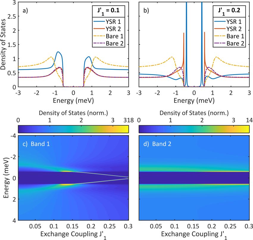
2
contrast to the real-valued energy independent BCS-type or-
der parameter.
In order to induce YSR states in the NbSe2 host, we have
doped the crystal with about 0.55% Fe [36]. Dopants that are
close to the surface can be directly seen in the topographic
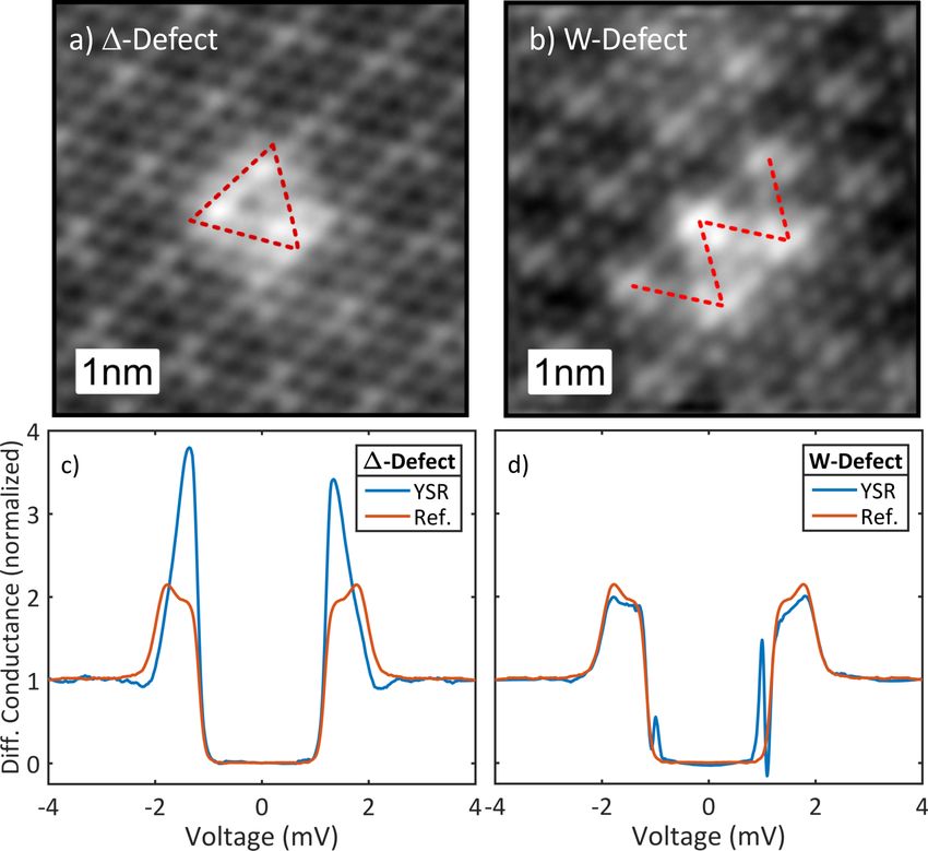
image shown in Fig. 1. We find two characteristic types of
impurities in our samples, which we attribute to Fe-defects:
one with a triangular (∆) shape (Fig. 1a) and one with a W-
shape (Fig. 1b). Both give rise to strong YSR states as can be
seen in the differential conductance spectra measured with a
superconducting vanadium tip in Fig. 1 c) and d), respectively.
However, the ∆-defect shows the YSR state inside the coher-
ence peaks (Fig. 1 c)), as can be seen by comparison with the
spectrum on the bare surface (red line). Indeed, the asymme-
try of the peak heights suggests the existence of YSR states
as opposed to a change of the local tunneling probability into
the two different bands. By contrast, the YSR state in Fig. 1d
appears close to the gap edge, but clearly inside the gap. Ev-
idently, these two types of YSR states substantially differ in
line width. The in-gap line width (Fig. 1d)) is much narrower
FIG. 1: Topography and differential conductance spectra of than the line width outside the gap (Fig. 1c)). These exper-
Fe in NbSe2 : Topographies of the two most common Fe impurities
having a triangular shape (∆) (a) and a W-shape (W) (b). The trian-
imental results present quite a different appearance of YSR
gular defect typically has a smaller exchange coupling so that the states than the “conventional” extremely narrow features oc-
YSR states appear within the coherence peaks (c). The W-defect has curring only inside the superconducting gap [37]. In the fol-
typically a higher exchange coupling and the YSR states commonly lowing, we will demonstrate that this is a direct consequence
appear inside the gap. An unperturbed reference spectrum with no of the energy dependent order parameter.
Fe impurity in the vicinity is shown in red. The current setpoint for Both topographic images in Fig. 1 show a rather regular,
the topography was 20 pA at a bias voltage of 100 mV, the setpoint
continuous lattice corrugation only modulated by a stronger
for the spectra was 200 pA at 4 mV.
density of states at the defect positions suggesting that the
impurities are buried very close to the surface, but not di-
rectly at or on the surface. For further analysis, we subtract
rectly related to the proximity-induced complex order pa-
an unperturbed reference spectrum of the bare surface, i. e.
rameters. Their imaginary parts are associated with relax-
with no impurities in the close vicinity of the YSR state, in
ation processes within the superconductor. The interaction
order to isolate the YSR states.
of an impurity with the individual bands in the bulk makes
these decay channels available to the YSR states. In this way,
we do not only demonstrate the relevance of intrinsic relax- The Order Parameters in Fe-doped NbSe2
ation channels for a certain class of robust quantum states,
but also establish YSR states as a probe for the imaginary part
In order to find a simple yet appropriate theoretical model,
of a complex-valued and energy dependent order parameter.
we need a detailed description of the order parameter in Fe-
doped NbSe2 . The doping of 0.55% of Fe atoms is already
strong enough to reduce the transition temperature from
Characterizing Fe-doped NbSe2 about 7.2 K [23, 38, 39] to 6.1 K [36], so that the effects of
the magnetic impurities on the bulk superconductor cannot
Layered NbSe2 is a two-band superconductor, whose bands be neglected. In order to theoretically describe the supercon-
interact via electron hopping between states near the Fermi ducting order parameter, we have to include the interaction
edge [18, 19, 23, 24, 28, 29, 31, 34, 35]. We follow the descrip- between the two bands [18, 19], as well as the interaction
tion by McMillan to model this mechanism [19]. Without the with a small but finite concentration of magnetic impurities
interband coupling, the first band is commonly assumed to [2, 40]. As we are analyzing density of states measurements
be superconducting, while the second is not [28]. Only the with no momentum information on the band structure nor on
interband coupling induces superconductivity in the second the order parameter, we refrain from employing models in-
band, which in turn reduces the order parameter in the first volving momentum dependent order parameters [22, 29, 33],
band. As a result, two energy dependent order parameters but instead focus on an effective description of the order pa-
emerge, which are complex-valued due to causality [20]. The rameter (for details, see the Supporting Information [36]). We
imaginary part can be interpreted as an intrinsic inverse life- add the selfenergies of the two interactions to the bare order
time due to the hopping between the bands. This stands in parameter ∆BCS1,2 for the first and second band, respectively.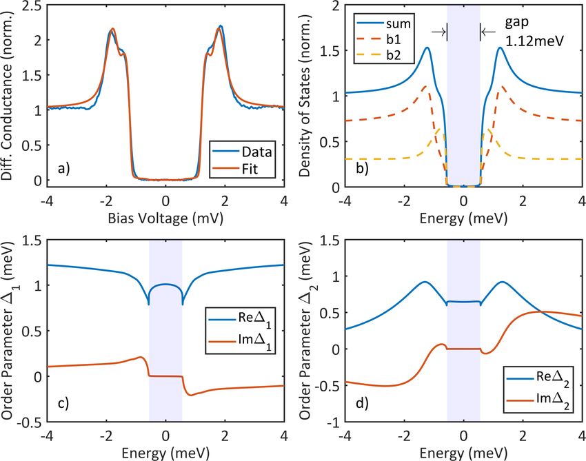
3
We find two coupled equations for the two order parameters
∆1,2 (ω) [41, 42]:
∆1 (ω) − ∆2 (ω) ∆1 (ω)
∆1 (ω) = ∆BCS
1 − Γ12 q − ζ1 q
∆22 (ω) − ω 2 ∆21 (ω) − ω 2
(1)
∆2 (ω) − ∆1 (ω) ∆2 (ω)
∆2 (ω) = ∆BCS
2 − Γ21 q − ζ2 q .
∆21 (ω) − ω 2 ∆22 (ω) − ω 2
Here, ω is the energy, Γ12 and Γ21 are the coupling param-
eters between the two bands and ζ 1,2 are the coupling con-
stants of the first and second band to the finite concentration
of magnetic impurities. The interband hopping as well as the
impurity interaction are proportional to the density of states
n 1,2 at the Fermi level of each band, so that the parameters in
Eq. 1 are related in the following way:
FIG. 2: Extracting the order parameters of Fe-doped NbSe2 : (a)
Γ21 ζ 1 n 1 Fit of the interband-impurity model to an unperturbed conductance
= = . (2) spectrum. The extracted fit parameters provide the input values for
Γ12 ζ 2 n 2
the subsequent analysis. (b) Calculated total density of states of the
superconducting substrate from the extracted fit parameters (sum).
Eq. 1 can be solved numerically using a multi-dimensional
The weighted density of states for band 1 (b1) and band 2 (b2) are
Newton-Raphson method. A more detailed discussion of shown as dashed lines. Note that the gap edges of both bands are
these equations is given in the Supporting Information [36]. at the same energy. (c) Resulting order parameter ∆1 (ω) of the first
The resulting normalized density of states ρ i (ω) of the i-th band. (d) Resulting order parameter ∆2 (ω) of the second band. The
band is blue shaded region indicates the gap.
ω
ρ i (ω) = Re q , (3) shown as dashed lines. Their gap edges lie at the same energy.
ω 2 − ∆i (ω)
2 The total density of states (solid line) features rather blunt co-
herence peaks, where shoulders indicate the coherence peaks
so that the total normalized density of states can be written of the second band. The gap itself is substantially narrower
as: (1.12 meV) than the bare BCS gap (2∆BCS 1 = 2.54 meV) (see
Supporting Information [36]). The corresponding order pa-
1+η 1−η
ρ(ω) = ρ 1 (ω) + ρ 2 (ω), (4) rameters are plotted in Fig. 2c) and d). For large energies the
2 2 real part of the order parameter for the first band shows an
where η is a ratio that accounts for the different densities of asymptotic approach to the ∆BCS 1 value of 1.27 meV, while the
states as well as the different tunneling probabilities into the imaginary part approaches zero. Inside the gap, the order pa-
two bands. Using the total density of states convolved with rameter is entirely real valued. In the vicinity of the coher-
the superconducting density of states of the V tip and with ence peaks, however, a strong energy dependence is visible.
the energy resolution function [43], we can fit the model to The order parameter of the second band approaches zero for
our experimental data. For details, see the Supporting Infor- large energies.
mation [36]. As a consequence, it becomes clear that for energies below
The resulting fit captures the experimental differential con- and around the coherence peaks, the real parts of the order
ductance quite accurately as shown in Fig. 2a). Following a parameters shown in Fig. 2c) and d) are larger than the energy
previous analysis [28], we have assumed a second band that of the gap edge (±0.55 meV). Because the energy position of
is intrinsically normal conducting, ∆BCS 2 = 0. The best fits the YSR state is directly related to the value of the order pa-
are obtained for a density of states ratio of n 1 /n 2 = 5, in rameter, we can already anticipate unconventional locations
agreement with previous assessments [28]. The unperturbed of the YSR states [17, 44].
order parameter for the first band ∆BCS1 = 1.27 meV is some-
what smaller than what has been reported for undoped NbSe2
(∆BCS,lit
1 = 1.4 meV, see Ref. 28 and references therein), but Magnetic impurity scattering of Fe in NbSe2
corresponds to roughly the same ratio as the reduction in the
transition temperature from 7.2 K to 6.1 K. For the coupling We now turn to the impurity scattering and calculate the
terms, we find Γ12 = 0.36 meV, ζ 1 = 57 µeV, and η = 0.38. YSR spectra following a simple T-matrix scattering formal-
The extracted density of states of Fe-doped NbSe2 is plotted ism [17]. In this approach, the superconducting host is de-
in Fig. 2b). The weighted individual densities of states are scribed by the normalized Green’s function for the two bands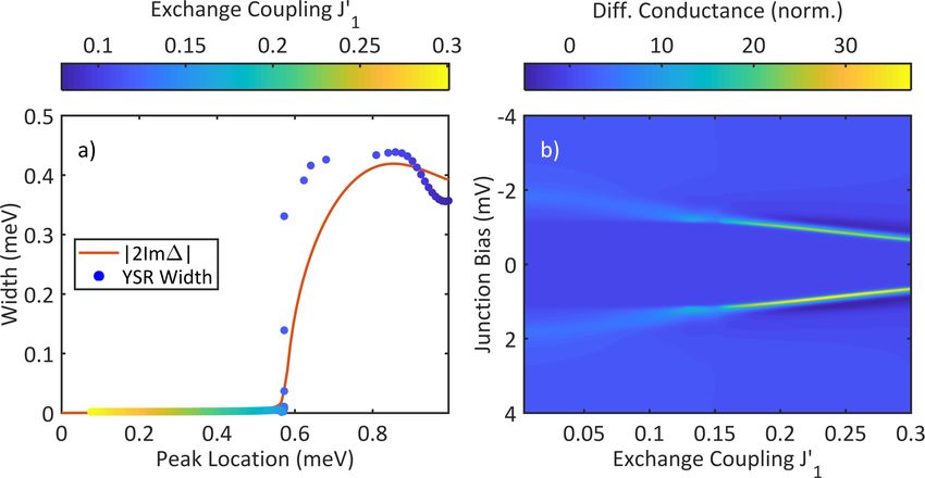
4

G 1,2 (ω):

                              1 ± η (ω + iΓ )σ0 − ∆1,2 (ω)σ1
             G 1,2 (ω) = −π                                  .    (5)
                                2
                                     q
                                       ∆2 (ω) − (ω + iΓ )2
                                         1,2

Here, the σi are the Pauli matrices in Nambu space with σ0
being the identity matrix. We add a Dynes-type parameter
Γ ≤ 5 µeV as a phenomenological lifetime broadening [15].
Larger values of Γ fill the gap, which is not observed in the
experiment. The T-matrix for the ith band can be written as

       Ti (ω) = Vi (1 − G i (ω)Vi )−1 with Vi = Ji0σ0 + Ui0σ3 ,   (6)

where Vi is the scattering potential with Ji0 = 12 JSni as
the dimensionless, effective magnetic exchange coupling and
Ui0 = U ni as the dimensionless, effective local Coulomb scat-
tering. Furthermore, 12 JS is the exchange coupling of a clas-
sical spin, U is the local Coulomb potential, and ni is the
density of states of the ith band at the Fermi level. The to-
tal Green’s function G iYSR (ω) can be written as:
                                                                        FIG. 3: Calculated YSR states: The solid lines correspond to the
                G iYSR (ω) = G i (ω) + G i (ω)Ti (ω)G i (ω).      (7)   YSR spectra coupling to band 1 (YSR 1) and band 2 (YSR 2), while the
                                                                        dashed lines represent the unperturbed spectra for the first (Bare 1)
For simplicity we only consider the total Green’s function              and second band (Bare 2), respectively. The ratio between the spec-
at the position of the impurity. Inserting the energy depen-            tra of the two bands correspond to the typical ratio η observed in the
                                                                        experiment. A small value for the Coulomb interaction U10 = 0.05
dent order parameters into Eq. 5, we can calculate the spectral
                                                                        and U20 = 0.01 = U10n 2 /n 1 has been chosen to make the spectrum
function Ai (ω) = − π1 tr{Im[G iYSR (ω)]} and thus the density of       asymmetric. (a) YSR spectrum for weak exchange coupling. The
states of the YSR resonances for different exchange couplings           YSR state is broad and within the region of the coherence peaks. (b)
Ji0.                                                                    Stronger coupling than (a), but still before the zero bias crossing. The
    The calculated YSR resonances for different exchange cou-           YSR state resides within the gap and has become extremely sharp.
plings J10 = (n 1 /n 2 )J20 are plotted in Fig. 3. For weak exchange    (c) and (d) YSR spectra vs. exchange coupling in band 1 and band 2,
coupling, the YSR state interacting with the first band can be          respectively. The color scaling is adapted to show the weaker fea-
                                                                        tures; it is non-linear for values larger than 3.5. The sharpening of
found within the coherence peaks (cf. Fig. 3a)). For stronger
                                                                        the peak as it enters the gap is clearly visible. In (d) the YSR peak
exchange coupling (but still below the zero energy crossing             develops much slower due to the reduced density of states in band
[6]), the YSR state for the first band moves into the gap and           2. For all panels, J10 /J20 = n 1 /n 2 .
becomes extremely sharp, as can be seen in Fig. 3b). Inside
the gap, the width of the YSR state is given by the parameter
Γ . In Fig. 3c) and d), the YSR spectra are shown as a func-            values are displayed in Fig. 4a) where the color coding repre-
tion of exchange coupling J 0 for the first and second band,            sents the strength of the exchange coupling J 0. The red line
respectively. With increasing coupling to the first band, the           in Fig. 4a) shows twice the imaginary part of the order pa-
YSR peaks shift towards zero energy and become extremely                rameter of the first band |2Im∆1 (ω)|.
narrow when entering the gap region.                                       We observe a clear correlation between the broadening of
    Apparently, the second band affects the YSR states much             the peak and the emergence of a finite Im∆1 (ω) as calculated
less, as can be seen in Figs. 3c) and d). Both bands have pre-          from Eq. 1. When the YSR peak position approaches the
dominantly Nb-d character [29, 31]. However, as the effective           coherence peaks, where |Im∆1 (ω)| increases abruptly, their
exchange coupling between the impurity and the supercon-                width increases abruptly as well. Thus, there is a clear indi-
ductor is proportional to the density of states in the supercon-        cation that the width of a YSR peak is related to the imaginary
ductor, i. e. J10/J20 = n 1 /n 2 , we may assume a strongly reduced     part of the superconducting order parameter.
impact of the second band. We, therefore, consider in leading
order only the YSR resonances in the first band.
    Due to the complicated shape of the YSR spectra, we re-                                          Discussion
strict the following analysis of the peaks to the peak position
and full width at half maximum. These quantities provide di-               In order to correlate the experimentally observed broad-
rect insight into the nature of the YSR state-bulk interaction.         ening of the YSR peak and its position with theory, we cal-
Keeping in mind that the peak position directly depends on              culate the differential conductance from the density of states
the strength of the exchange coupling (Fig. 3), the extracted           following Eq. 7. The resulting spectra are shown in Fig. 4b)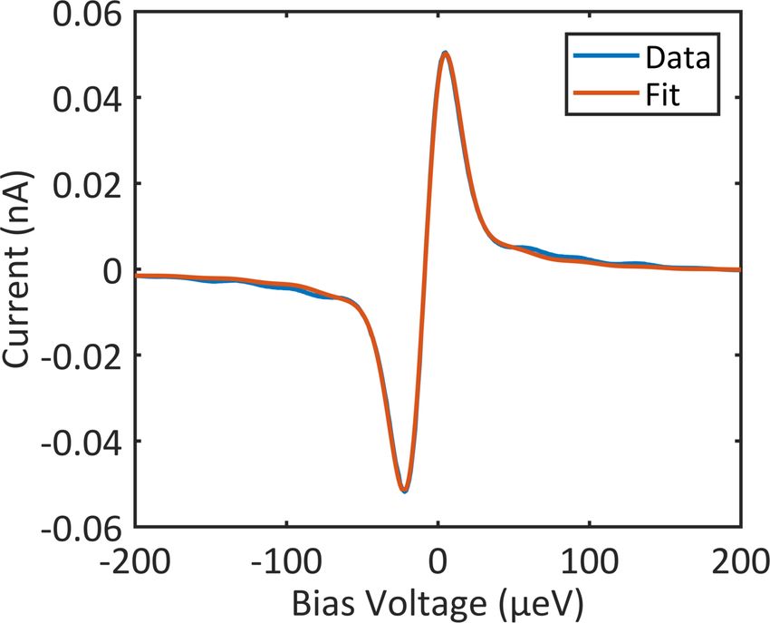
5

                                                                       as a function of exchange coupling J10. The sharpening of the
                                                                       peaks when entering the region of the gap is still clearly visi-
                                                                       ble even though now the width of the YSR peaks is limited
                                                                       by the energy resolution of the STM [43]. Two represen-
                                                                       tative spectra of YSR states outside and inside the gap are
                                                                       plotted in Fig. 5a) and b), respectively. An unperturbed, aver-
                                                                       aged reference spectrum was subtracted to better isolate the
                                                                       YSR states. These experimental spectra can be compared to
                                                                       Fig. 5c) and d) showing two slices from Fig. 4b) with similar
                                                                       peak positions as in Fig. 5a) and b), respectively. The calcu-
                                                                       lated spectra are normalized to the normal state conductance
                                                                       and scaled with the ratio η (cf. Eq. 4). The substraction of an
FIG. 4: Evolution of the YSR peak width: (a) YSR peak width
vs. peak location. The width becomes extremely narrow in the re-       unperturbed reference spectrum is not necessary in the cal-
gion of the superconducting gap. The color coding represents the       culated spectra, because the coherence peaks are suppressed
strength of the exchange coupling. The red line is twice the imag-     on the impurity site. Selecting theory spectra with match-
inary part of the order parameter ∆1 (ω) of the first band. We see     ing peak positions, we observe good agreement between the
a clear correlation between the peak width and the imaginary part.     corresponding panels concerning the width of the YSR peaks
(b) Differential conductance calculated from the YSR spectral func-    as well as their overall shape. We find, however, a reduced
tion and the density of states of the superconducting V tip as well
                                                                       height in the experimental peaks, which we attribute to the
as finite energy resolution. The sharpening of the YSR state when
entering the gap, is clearly visible.                                  measurement slightly above the (subsurface) impurity. Away
                                                                       from the scattering center of the impurity, intensity modula-
                                                                       tions can strongly reduce the peak height [30]. We assume
                                                                       that they do not affect the peak position nor their width. In-
                                                                       terestingly, the asymmetry of the YSR peaks is different in
                                                                       Fig. 5a) and b), which indicates a different Coulomb scatter-
                                                                       ing potential U 0 (assuming that the particle-hole asymmetry
                                                                       in the lattice Green’s function does not change significantly
                                                                       between the impurities).
                                                                          From each of the experimental and theoretical spectra, we
                                                                       extract the YSR peak widths and positions as indicated in Fig.
                                                                       5a)-d) and display them in Fig. 5e). Excellent agreement is
                                                                       seen between the experimentally extracted values and the
                                                                       calculated spectra, indicating that there is indeed a strong
                                                                       correlation between the shape and position of the YSR states
                                                                       and the details of the underlying order parameter. Although
                                                                       W-defects seem to couple stronger than ∆-defects, both de-
                                                                       fects can be found in a range of exchange couplings (probably
                                                                       due to slightly different local environments), such that either
                                                                       defect can be used independently to infer the relation of the
                                                                       width to the imaginary part of the order parameter.
                                                                          We establish a nontrivial relation between the order pa-
                                                                       rameter and the energy position of YSR states in Fe-doped
                                                                       NbSe2 . In contrast, for an energy independent BCS order pa-
                                                                       rameter (which by causality carries at most a constant imagi-
                                                                       nary part [20]), the YSR state always lies within the supercon-
                                                                       ducting gap, because the order parameter in this case defines
                                                                       the position of the gap edge. However, interband coupling
FIG. 5: Comparison of experiment with theory: Peak positions
and widths indicated for YSR states outside the gap in (a) and in-
                                                                       induces energy dependent order parameters. As a result, the
side the gap in (b), where an unperturbed reference spectrum was       actual edges of the superconducting gaps are at a smaller en-
subtracted. In (c) and (d), the corresponding calculated spectra are   ergy than the values of the order parameters. Consequently,
given. (e) Experimental YSR peak widths vs. peak position in com-      YSR resonances may appear at energies outside the gap and
parison with the extracted YSR peak widths from the calculated dif-    inside the coherence peaks. If the exchange coupling is too
ferential conductance spectra. The W-shaped defect and the trian-      small, then the YSR state cannot be distinguished from the
gular defect (∆) are color coded in blue and red, respectively. The    unperturbed coherence peaks anymore and are experimen-
blue shaded region indicates the sample gap.
                                                                       tally inaccessible.
                                                                          The spectral functions on which these arguments are
6
based, result from the imaginary parts of respective Green’s as a “rephrased” selfenergy, where its imaginary part is con-
functions. They are commonly interpreted as single particle nected to lifetime broadening. In this way, we have shown
excitation spectra with widths associated with relaxation into that YSR states may couple to intrinsic relaxation channels.
ground states. Here, the imaginary part of the order param- While we have analyzed this behavior on a simple, well-
eter can be interpreted as a measure for the effective lifetime known s-wave superconductor, we expect similar or even
of YSR resonances, not to be mistaken for its phase. In fact, more complex interactions of YSR states with unconventional
the imaginary part considered here renders the Green’s func- (d-wave, p-wave), proximity-induced, and/or topological su-
tion non-Hermitian, thus indicating effectively energy dissi- perconductors. At the same time, we have demonstrated that
pation. In the case of NbSe2 , these relaxation processes must YSR states may serve as sensitive probes for the complex-
be attributed to hopping between the two bands in the bulk valued order parameter, which opens up new possibilities for
material that participate in the superconductivity. The Fe- understanding the intricacies of multi-band superconductiv-
doping additionally contributes to the relaxation with hop- ity as well as unconventional superconductors.
ping to the small concentration of impurities. These relax-
ation processes are, of course, strongest when the YSR state is
located within the coherence peaks where the order parame- Acknowledgements
ter has a finite imaginary part. They sharpen up considerably
within the superconducting gap, where the order parameter We gratefully acknowledge stimulating discussions with
becomes (almost) real and there are (almost) no relaxation Wolfgang Belzig, Hans Boschker, Carlos Cuevas, Reinhard
channels. In this regime, the experimental width is limited Kremer, Bettina Lotsch, Jochen Mannhart, Fabian Pauly, and
by the resolution of our STM, which is determined by the in- Markus Ternes. This work was funded in part by the ERC
teraction of the tunneling quasiparticles with the local elec- Consolidator Grant AbsoluteSpin and by the Center for In-
tromagnetic environment according to the P(E)-description tegrated Quantum Science and Technology (IQST ). CRV ac-
[43, 45, 46]. knowledges funding from the COST Action ECOST-STSM-
This finite energy resolution of the STM obscures a direct CA15128-010217-082276. SD acknowledges financial support
observation of the peak width inside the superconducting from the Carl-Zeiss-Stiftung.
gap. The full width at half maximum of the energy resolution
function is dominated by the fluctuations of single charges at
the junction capacitance [43] and is usually much broader
than the intrinsic peak width of just a few µeV. Nevertheless,
∗ Corresponding author; electronic address: c.ast@fkf.mpg.de
we surmise that even in the gap, there can be weak couplings
to inelastic relaxation processes, which may be modeled ef- [1] Yu, L. Acta Phys. Sin. 21, 75 (1965).
fectively by a generic imaginary constant selfenergy, such as [2] Shiba, H. Prog. Theor. Phys. 40, 435 (1968).
[3] Rusinov, A. I. JETP Lett. 9, 85 (1969).
the Dynes parameter [15]. [4] Yazdani, A., Jones, B. A., Lutz, C. P., Crommie, M. F., and Eigler,
Turning the argument around, we find that the YSR states D. M. Science 275, 1767 (1997).
can be exploited as probes of complex-valued order parame- [5] Hudson, E. W., Lang, K. M., Madhavan, V., Pan, S. H., Eisaki,
ters in the range where they can exist. For a deeper quan- H., Uchida, S., and Davis, J. C. Nature 411, 920 (2001).
titative analysis, one has to consider also the (weak) local [6] Franke, K. J., Schulze, G., and Pascual, J. I. Science 332, 940
modifications of the order parameter induced by the YSR (2011).
[7] Ruby, M., Peng, Y., von Oppen, F., Heinrich, B. W., and Franke,
states themselves [17, 47]. Thus, using YSR states as probes
K. J. Phys. Rev. Lett. 117, 186801 (2016).
for the complex part of the superconducting order parame- [8] Nadj-Perge, S., Drozdov, I. K., Bernevig, B. A., and Yazdani, A.
ter could give valuable insight into the superconductivity of Phys. Rev. B 88, 020407 (2013).
other non-trivial materials, especially those of an unconven- [9] Nadj-Perge, S., Drozdov, I. K., Li, J., Chen, H., Jeon, S., Seo, J.,
tional, proximity-induced, or topological nature. MacDonald, A. H., Bernevig, B. A., and Yazdani, A. Science 346,
602 (2014).
[10] Ruby, M., Pientka, F., Peng, Y., von Oppen, F., Heinrich, B. W.,
Conclusion and Franke, K. J. Phys. Rev. Lett. 115, 197204 (2015).
[11] Ménard, G. C., Guissart, S., Brun, C., Leriche, R. T., Trif, M.,
Debontridder, F., Demaille, D., Roditchev, D., Simon, P., and
In summary, we have shown that complex-valued en- Cren, T. Nature Commun. 8, 2040 (2017).
ergy dependent order parameters as they can result from [12] Balatsky, A. V., Vekhter, I., and Zhu, J.-X. Rev. Mod. Phys. 78,
multi-band superconductivity give rise to nontrivial inter- 373 (2006).
actions with local pair-breaking potentials. The resulting [13] Heinrich, B. W., Braun, L., Pascual, J. I., and Franke, K. J. Nat.
YSR states may not just exist in the superconducting gap, Phys. 9, 765 (2013).
[14] Ruby, M., Pientka, F., Peng, Y., von Oppen, F., Heinrich, B. W.,
but also inside the coherence peaks (outside the gap), where and Franke, K. J. Phys. Rev. Lett. 115, 087001 (2015).
they acquire a substantial broadening due to dissipative re- [15] Dynes, R. C., Narayanamurti, V., and Garno, J. P. Phys. Rev.
laxation processes into the continuum. These processes are Lett. 41, 1509 (1978).
expressed in the order parameter, which can be interpreted [16] Martin, I. and Mozyrsky, D. Phys. Rev. B 90, 100508 (2014).7
[17] Salkola, M. I., Balatsky, A. V., and Schrieffer, J. R. Phys. Rev. B Pons, S., Debontridder, F., Roditchev, D., Sacks, W., Cario, L.,
55, 12648 (1997). Ordejón, P., Garcı́a, A., and Canadell, E. Phys. Rev. B 92, 134510
[18] Suhl, H., Matthias, B. T., and Walker, L. R. Phys. Rev. Lett. 3, (2015).
552 (1959). [32] Ptok, A., G lodzik, S., and Domański, T. Phys. Rev. B 96, 184425
[19] McMillan, W. L. Phys. Rev. 175, 537 (1968). (2017).
[20] Toll, J. S. Phys. Rev. 104, 1760 (1956). [33] Galvis, J.A., Herrera, E., Berthod, C., Vieira, S., Guillamón, I.,
[21] Hess, H. F., Robinson, R. B., and Waszczak, J. V. Phys. Rev. Lett. and Suderow, H. arXiv:1711.09269 (2017).
64, 2711 (1990). [34] Dvir, T., Massee, F., Attias, L., Khodas, M., Aprili, M., Quay, C.
[22] Hayashi, N., Ichioka, M., Machida, K. Phys. Rev. B 56, 9052 H. L., and Steinberg, H. Nature Commun. 9, 598 (2018).
(1997). [35] Machida, K. and Shibata, F. Prog. Theor. Phys. 47, 1817 (1972).
[23] Yokoya, T., Kiss, T., Chainani, A., Shin, S., Nohara, M., and Tak- [36] see Supporting Information.
agi, H. Science 294, 2518 (2001). [37] Heinrich, B. W., Pascual, J. I., and Franke, K. J. arXiv:1705.03672
[24] Rodrigo, J. and Vieira, S. Physica C: Supercond. 404, 306 (2004). (2017).
[25] Kohen, A., Proslier, T., Cren, T., Noat, Y., Sacks, W., Berger, H., [38] Frindt, R. F. Phys. Rev. Lett. 28, 299 (1972).
and Roditchev, D. Phys. Rev. Lett. 97, 027001 (2006). [39] Revolinsky, E., Spiering, G. A., and Beerntsen, D. J. J. Phys.
[26] Guillamon, I., Suderow, H., Guinea, F., and Vieira, S. Phys. Rev. Chem. Solids 26, 1029 (1965).
B 77, 134505 (2008). [40] Maki, K. Prog. Theor. Phys. 32, 29 (1964).
[27] Kimura, H., Barber, R. P., Ono, S., Ando, Y., and Dynes, R. C. [41] Zarate, H. G. and Carbotte, J. P. J. Low Temp. Phys. 59, 19 (1985).
Phys. Rev. B 80, 144506 (2009). [42] Golubov, A. A. and Mazin, I. I. Phys. Rev. B 55, 15146 (1997).
[28] Noat, Y., Cren, T., Debontridder, F., Roditchev, D., Sacks, W., [43] Ast, C. R., Jäck, B., Senkpiel, J., Eltschka, M., Etzkorn, M.,
Toulemonde, P., and San Miguel, A. Phys. Rev. B 82, 014531 Ankerhold, J., and Kern, K. Nature Commun. 7, 13009 (2016).
(2010). [44] Flatté, M. E. and Byers, J. M. Phys. Rev. B 56, 11213 (1997).
[29] Rahn, D. J., Hellmann, S., Kalläne, M., Sohrt, C., Kim, T. K., [45] Devoret, M. H., Esteve, D., Grabert, H., Ingold, G., Pothier, H.,
Kipp, L., and Rossnagel, K. Phys. Rev. B 85, 224532 (2012). and Urbina, C. Phys. Rev. Lett. 64, 1824 (1990).
[30] Ménard, G. C., Guissart, S., Brun, C., Pons, S., Stolyarov, V. S., [46] Averin, D., Nazarov, Y., and Odintsov, A. Physica B: Cond. Matt.
Debontridder, F., Leclerc, M. V., Janod, E., Cario, L., Roditchev, 165-166, 945 (1990).
D., Simon, P., and Cren, T. Nature Phys. 11, 1013 (2015). [47] Flatté, M. E. and Byers, J. M. Phys. Rev. Lett. 78, 3761 (1997).
[31] Noat, Y., Silva-Guillén, J. A., Cren, T., Cherkez, V., Brun, C.,8
Supplementary Information
Tip and Sample Preparation of the crystals was confirmed with X-ray diffraction and EDX,
respectively. The Fe content was too low to be detected in the
The experiments were carried out in a scanning tunneling EDX. The magnetic properties were measured on a MPMS
microscope (STM) operating at a base temperature of 15 mK (magnetic properties measurements system) from Quantum
[1]. The sample that was used was an 0.55% Fe-doped NbSe2 Design. From the MPMS measurements, we find an onset
single crystal. To obtain a clean surface, the sample was transition temperature TC = 6.1 K (see Fig. S1).
cleaved with scotch tape in ultrahigh vacuum. The tip ma- A topographic overview map of the Fe-doped NbSe2
terial was a polycrystalline vanadium wire, which was cut in surface can be seen in Fig. S2. A statistical distribution of
air and prepared in ultrahigh vacuum by sputtering and field subsurface Fe atoms is visible. The YSR spectra were taken
emission. at the geometric center of the defect.
Fe-doped NbSe2
Calculating the differential Conductance
Single crystals of Fe-doped NbSe2 were grown with chem-
ical vapor transport. Powders of Nb and Fe in a ratio The differential conductance dI /dV was calculated from
of 99.45:0.55 were mixed well and then placed in a quartz the tunneling current
tube. Se chips were added in a stoichiometric ratio to yield
Nb0.9945 Fe0.055 Se2 . Iodine was used as the transport agent. I (V ) = e Γ(V ® ) ,
® ) − Γ(V (8)
The sealed tube was heated to 900◦ C with a temperature gra-
dient of 75◦ C for three weeks. The structure and composition with the tunneling probability from tip to sample
∫∞ ∫∞
® )= 1
Γ(V dEdE 0 ρ t (E)ρ s (E 0 + eV )f (E)[1 − f (E 0 + eV )]P(E − E 0). (9)
e 2R T
−∞ −∞
The other tunneling direction Γ(V ® ) from sample to tip can be blockade and as such can be well described by the P(E)-
obtained by exchanging electrons and holes in Eq. 9. Here, theory [4–6]. The current-voltage characteristics I (V ) for the
R T is the tunneling resistance, f (E) = 1/(1 + exp(E/k BT )) is Josephson effect is given by
the Fermi function, and ρ t , ρ s are the densities of states of tip
and sample, respectively. The P(E)-function describes the ex-
change of energy with the environment during the tunneling πeE J2
I (V ) = [P(2eV ) − P(−2eV )] , (10)
process and is interpreted as the energy resolution function ~
of the STM [2].
The parameter η introduced in the main text weighs the where E J is the Josephson coupling energy and e is the electric
density of states of the two bands in NbSe2 as they appear charge. The experimental data and the corresponding fit are
in the experimental differential conductance spectra. It in- shown in Fig. S3. The details of the P(E)-function pertaining
cludes both the density of states for each band as well as the to the tunnel junction of a scanning tunneling microscope are
tunneling probability into each band. As it is not necessary given elsewhere [3]. The relevant fitting parameters for the
to separate these contributions in this analysis, we have com- P(E)-function are the tunnel junction capacitance C J = 9.5 fF
bined them with the density of states. This allows us to use and an effective temperature T = 100 mK. The environmental
Eq. 9 with an overall tunneling resistance R T , which can be impedance is modeled by a finite transmission line having an
directly determined from the experimental data. environmental resistance of R env = 377 Ω, a tip resonance
energy of ~ωres = 45 µeV, and a resonance broadening factor
For the parameters in the P(E)-function, we perform an in-
α = 0.7. With these parameters, we can use the P(E)-function
dependent fit of a Josephson spectrum with the same macro-
as the energy resolution function.
scopic tip as used for the other spectra presented here [3]. The
Josephson effect in a scanning tunneling microscope at very The density of states of the tip ρ t was modeled by the Maki
low temperatures is governed by the dynamical Coulomb equation [8, 9] because of the intrinsic magnetic impurities in9
vanadium:
ω + iΓt
ρ t (ω) = Re q , (11)
(ω + iΓt )2 − ∆t (ω)
2
with
∆t (ω)
∆t (ω) = ∆BCS
t − ζt q . (12)
∆2t (ω) − ω 2
Here, Γt is a phenomenological broadening term and ζ t is a
depairing parameter due to the interaction with a small con-
centration of magnetic impurities. For the vanadium tip, we
FIG. S1: Zero-field cooled (ZFC) and field cooled (FC) susceptibility
curves of the Fe-doped NbSe2 . The onset transition temperature is find ∆BCS
t = 710 µeV, Γt = 5 µeV and ζ t = 33 µeV. Note that
about 6.1 K. The field cooled values are higher than the zero-field due to the magnetic interaction modeled by the Maki equa-
cooled values indicating a type-II superconductor. tion, the tip gap (2 × 550 µeV) is smaller than twice the order
parameter of vanadium (2 × 710 µeV).
Differential conductance spectra were recorded with a
lock-in amplifier having a modulation amplitude of 20 µV and
a modulation frequency of 793 Hz. The resulting broadening
is also included in the analysis and enters the calculated dif-
ferential conductance spectra through an additional convo-
lution.
Momentum dependent vs. energy dependent order
parameters
At the heart of BCS theory, lies a potentially momentum
dependent order parameter ∆k , which appears in the mo-
mentum and energy dependent Green’s function [10]:
1
G(ω, k) = (13)
ωσ0 − εk σ3 − ∆k σ1
FIG. S2: Topographic overview map of the Fe-doped NbSe2 surface.
A statistical distribution of subsurface Fe atoms is visible. The cur- Integrating over momentum space yields a momentum inde-
rent setpoint was 20 pA at a bias voltage of 100 mV. pendent Green’s function, where the functional dependence
of the order parameter is projected onto an energy scale re-
sulting in an energy dependent order parameter ∆(ω) [7, 10],
ωσ0 − ∆(ω)σ1
G(ω) = −π p , (14)
∆2 (ω) − ω 2
which has been used in the main text. In this sense, the mo-
mentum dependent order parameter ∆k is related to the en-
ergy dependent order parameter ∆(ω) like the band structure
εk is related to the density of states n(ω). As such, using an
energy dependent order parameter does not ultimately ex-
clude a momentum dependence, it even implies it. In our
STM measurements, we are dealing with density of states
measurements having no direct information of the momen-
tum dependence. We, therefore, have chosen the simplest,
FIG. S3: Current-voltage characteristics of the Josephson effect (blue suitable model to describe our experimental data since the
curve) fitted with the P(E)-theory (red curve) to extract the parame- extended complexity of employing a momentum dependent
ters describing the P(E)-function. The spectrum was measured with
order parameter may change some details [11–13], but not
a current setpoint of 15 nA at a bias voltage of 4 mV.
the general message of the manuscript.10
Numerical Solution for ∆1 (ω) and ∆2 (ω) where J (®
y) is the Jacobian matrix of f (®
y) with
∂ fi
For a numerical solution at arbitrary energies, it is conve- J (®
y)i j = (23)
∂y j
nient to work with dimensionless quantities. We define
The next iteration value is then
ω ω
u1 = u2 = . (15) y®n+1 = y®n + ∆y®n . (24)
∆1 (ω) ∆2 (ω)
When calculating the values y® as function of energy ω, the
Using also the dimensionless abbreviations best starting point is ω = 0 and then to use the previous
ω Γ12 Γ21 value as the starting point for the next value of ω. A universal
ω̃ = ; Γ˜12 = BCS ; Γ˜21 = BCS ; starting point for ω = 0 is y® = (0, 1, 0, 1), which works well
∆BCS
1 ∆ 1 ∆ 1 for a broad set of parameters.
ζ1 ζ2 ∆BCS
ζ˜1 = BCS ; ζ˜2 = BCS ; δ = 2BCS , (16) Analysis of the coupled two-band superconductivity
∆1 ∆1 ∆1
Eq. 1 transforms into We start from McMillan’s coupled equations for a two-
band superconductor with bare (energy independent and
u2 − u1 u1 real-valued) BCS gaps ∆BCS ≡ ∆0 , 0 and ∆BCS = 0, re-
ω̃ = u 1 − Γ˜12 q − ζ˜1 q (17) 1 2
1 − u 22 1 − u 12 spectively, i.e.
u1 − u2 u2 ∆1 (ω) − ∆2 (ω)
ω̃ = u 2δ − Γ˜21 q − ζ˜2 q . (18) ∆1 (ω) = ∆0 − Γ12 q (25)
1 − u 12 1 − u 22 ∆22 − ω 2
∆2 (ω) − ∆1 (ω)
We have referenced all variables to ∆BCS ∆2 (ω) = −Γ21 . (26)
1 , because if we were
q
to reference each equation to its own order parameter, the ∆21 − ω 2
problem becomes ill-defined, if ∆BCS
2 = 0. Avoiding this prob- Here Γ12 , Γ21 denote interband coupling rates. The second
lem allows us to work with dimensionless quantities. For the equation can be easily solved to read
Newton-Raphson method, we have to cast the above equa-
tions into a different form defining Γ21 ∆1
∆2 = q (27)
u1 1 u2 1 Γ21 + ∆21 − ω 2
y1 = q ; y2 = q ; y3 = q ; y4 = q
1 − u 12 1 − u 12 1 − u 22 1 − u 22 which means that a complex-valued ∆1 implies a complex-
valued ∆2 and vice versa.
(19)
Now, in case of NbSe2 one may approximately assume
We find
Γ12
Γ21 ∼ ∆0 which means that ∆0 ∼ ∆1 ∼ ∆2 as long
y1 − Γ˜12 (y3y2 − y1y4 ) − ζ˜1y1y2 − ω̃y2 = 0 as only orders of magnitude are concerned. Accordingly, one
writes ∆1 = ∆0 + δ 1 with |δ 1 | ∼ Γ12
∆0 and solves the first
δy3 − Γ˜21 (y1y4 − y3y2 ) − ζ˜2y3y4 − ω̃y4 = 0
equation in (26) for δ 1 , i.e.,
y22 − y12 − 1 = 0
∆0 − ∆2
y42 − y32 − 1 = 0 (20) δ 1 = −Γ12 q (28)
Γ12 + ∆22 − ω 2
These equations can be easily solved using a multi-
dimensional Newton-Raphson method [15, 16]. while for (27) one obtains by putting ∆1 ≈ ∆0
To solve the system of equations in Eq. 20, we de- Γ21 ∆0
∆2 = . (29)
fine a multi-valued function f (® y), whose input is a four-
q
Γ21 + ∆20 − ω 2
dimensional vector y® = (y1 , y2 , y3 , y4 ) and whose output are
the values of the four quantities on the left hand sides in Eq. Using this latter result, one finds the explicit expression for
20. With the Newton-Raphson method, we seek a physical the correction to ∆1 to read
solution to the equation q
∆0 Γ12 ∆20 − ω 2
f (®
y) = 0. (21) δ1 = − q r q .
Γ12 (Γ21 + ∆20 − ω 2 ) + Γ21
2 ∆2 − ω 2 (Γ +
0 21 ∆20 − ω 2 )2
This is done iteratively by calculating the next value from the
equation (30)
One can now distinguish three regions in frequency
f (®
yn ) + J (®
yn ) · ∆y®n = 0 ⇒ ∆y®n = −J (®
yn )−1 f (®
yn ) (22) space:11
1. |ω| < ωc
Here, ωc = α ∆0 , where α < 1 is the√positive solution of α 3 +
α 2 +ϵ 2 α −ϵ 2 = 0 with ϵ = Γ21 /∆0 ≈ 2. The only real solution ∗ Corresponding author; electronic address: c.ast@fkf.mpg.de
is α ≈ 0.65. In this regime, ∆1 , ∆2 are both real-valued with [1] M. Assig, et al., Rev. Sci. Instr. 84, 033903 (2013).
∆1 , ∆2 > 0. The energy ωc defines the threshold, below which [2] Ast, C. R., et al., Nature Communications 7, 13009 (2016).
imaginary parts in both order parameters are absent. Thus ωc [3] Jäck, B., et al., Appl. Phys. Lett. 106, 013109 (2015).
determines the width of the superconducting gap. Note that [4] Devoret, M. H., Esteve, D., Grabert, H., Ingold, G., Pothier, H.,
the gap widths for both bands are identical as an imaginary and Urbina, C. Phys. Rev. Lett. 64, 1824 (1990).
part in one order parameter induces an imaginary part in the [5] Averin, D. V., Nazarov, Yu. V., and Odintsov, A. A., Physica B:
Cond. Mat. 165, 945 (1990).
other one and vice versa.
[6] Ingold, G., Grabert, H., and Eberhardt, U. Phys. Rev. B 50, 395
2. ωc < |ω| . ∆0 (1994).
In this regime, δ 1 is complex-valued so that also ∆2 ac- [7] W. L. McMillan, Phys. Rev. 175, 537 (1968).
quires a small imaginary part. The root is taken according to [8] K. Maki, Prog. Theor. Phys., 32, 29 (1964).
√ √
ωc − ω → −i ω − ωc . Accordingly, Im{δ 1 (ω > 0)} < 0 so [9] H. Shiba, Progress of Theoretical Physics, 40, 435 (1968).
that Im{∆2 (ω > 0)} < q0. In particular, ∆2 (ωq [10] J. R. Schrieffer, “Theory of Superconductivity”, Advances Book
c ) ≈ −0.65 ∆0
Classics, Perseus Books (1999).
while δ 1 (ωc )/∆0 = − ∆20 − ωc2 /[Γ12 (Γ21 + ∆20 − ωc2 )] ≈ [11] Hayashi, N., Ichioka, M., Machida, K. Phys. Rev. B 56, 9052
−0.349 ∆0 . Note that this perturbative treatment is less ac- (1997).
curate near the boundaries of their respective frequency do- [12] Rahn, D. J., Hellmann, S., Kalläne, M., Sohrt, C., Kim, T. K.,
Kipp, L., and Rossnagel, K. Phys. Rev. B 85, 224532 (2012).
mains.
[13] Galvis, J.A., Herrera, E., Berthod, C., Vieira, S., Guillamón, I.,
3. ∆0 . |ω| and Suderow, H. arXiv:1711.09269 (2017).
In this regime, Im{δ 1 } and ∆2 approach zero and Im{∆2 (ω > [14] R. C. Dynes, V. Narayanamurti, and J. P. Garno, Phys. Rev. Lett.
0)} > 0 meaning that Im{∆2 } = 0 at a frequency near ∆0 . 41, 1509 (1978).
The above treatment can be refined by replacing ∆0 → [15] D. C. Worledge and T. H. Geballe, Phys. Rev. B 62, 447 (2000).
∆0 + δ 1 in (29) and using the expression (30). One then finds [16] F. S. Action, “Numerical Methods That Work”, Washington:
Mathematical Association of America (1979).
∆2 (ωc ) ≈ ∆1 (ωc ) in agreement with the full numerical solu-
tion (see Fig. 2).You can also read