A Gaussian-Process-Based Global Sensitivity Analysis of Cultivar Trait Parameters in APSIM-Sugar Model: Special Reference to Environmental and ...
←
→
Page content transcription
If your browser does not render page correctly, please read the page content below
agronomy
Article
A Gaussian-Process-Based Global Sensitivity
Analysis of Cultivar Trait Parameters in APSIM-Sugar
Model: Special Reference to Environmental and
Management Conditions in Thailand
W. B. M. A. C. Bandara 1,2, * , Kazuhito Sakai 1,3, *, Tamotsu Nakandakari 1,3 , Preecha Kapetch 4
and R. H. K. Rathnappriya 1
 1   Faculty of Agriculture, University of the Ryukyus, 1 Senbaru, Nishihara-cho, Okinawa 903-0213, Japan;
     zhunai@agr.u-ryukyu.ac.jp (T.N.); himashakithminir@gmail.com (R.H.K.R.)
 2   Department of Agricultural Engineering, Faculty of Agriculture, University of Ruhuna,
     Kamburupitiya 81100, Sri Lanka
 3   United Graduate School of Agricultural Sciences, Kagoshima University, 1-21-24 Korimoto, Kagoshima-shi,
     Kagoshima 890-0065, Japan
 4   Nakhon Sawan Agricultural Research and Development Center, Moo 2, Udomthanya, Takfa 60190, Thailand;
     p.kapetch@gmail.com
 *   Correspondence: chathu.anushk@gmail.com or cbandara@ageng.ruh.ac.lk (W.B.M.A.C.B.);
     ksakai@agr.u-ryukyu.ac.jp (K.S.)

 Received: 22 June 2020; Accepted: 7 July 2020; Published: 9 July 2020

 Abstract: Process-based crop models are advantageous for the identification of management strategies
 to cope with both temporal and spatial variability of sugarcane yield. However, global optimization
 of such models is often computationally expensive. Therefore, we performed global sensitivity
 analysis based on Gaussian process emulation to evaluate the sensitivity of cane dry weight to trait
 parameters implemented in the Agricultural Productions System Simulator (APSIM)-Sugar model
 under selected environmental and management conditions in Khon Kaen (KK), Thailand. Emulators
 modeled 30 years, three soil types and irrigated or rainfed conditions, and emulator performance was
 investigated. rue, green_leaf_no, transp_eff_cf, tt_emerg_to_begcane and cane_fraction were identified
 as the most influential parameters and together they explained more than 90% of total variance on
 the simulator output. Moreover, results indicate that the sensitivity of sugarcane yield to the most
 influential parameters is affected by water stress conditions and nitrogen stress. Our findings can be
 used to improve the efficiency and accuracy of modeling and to identify appropriate management
 strategies to address temporal and spatial variability of sugarcane yield in KK.

 Keywords: APSIM; Gaussian process emulation; global sensitivity analysis; sugarcane

1. Introduction
     Sugarcane plays a critical role in Thailand’s economy and has become one of the most important
agricultural crops of the country [1]. Being the major sugarcane production region of Thailand, the
Northeast is responsible for 43.2% of the total produced sugarcane and 44.2% of the total sugarcane
harvesting area [2]. Recently, paddy fields that produce lower net value per hectare in the Khon Kaen
(KK) area of the Northeast have been converted into sugarcane fields [3]. Increasing evidence indicates
that global climate change could reduce sugarcane production. According to Preecha et al. [4], climate
change is the most obvious factor responsible for spatial and temporal yield variability in the Northeast
of Thailand. Thus, identification of suitable management strategies to cope with both temporal and

Agronomy 2020, 10, 984; doi:10.3390/agronomy10070984                         www.mdpi.com/journal/agronomy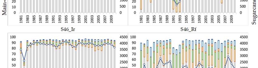
Agronomy 2020, 10, 984                                                                             2 of 16

spatial variability is of a paramount importance. For instance, sugar mills require forecasting and
estimation of cane yield to manage their strategies.
     In this respect, it is advantageous to study how different cultivars perform under different
environmental and management conditions. Process-based crop models that can simulate cultivar
differences are used by researchers to simulate how the cultivars perform under various production
environments and to identify advantageous traits in defined environments [5]. However, recent
advances in crop models for cultivar–environment interaction studies have created a requirement for
quantifying and analyzing uncertainty in crop models. For instance, Ojeda et al. [6] has quantified
the input uncertainty for their study on assessing effect of data aggregation in regional scale crop
modeling. Sensitivity analysis (SA) is useful in studying how the uncertainty of the model input
affects the uncertainty of the model output and to what extent model outputs are sensitive to model
parameters [7].
     Song et al. [8] suggested a way of dividing SA into local and global SA. Local one-at-a-time
sensitivity indices are efficient if linear output responses are produced by all the factors in a model.
In general, as explained by Ewert et al. [9] variations in input factors generate non-linear model output
responses. Therefore, an alternative global SA (GSA) approach is required, in which the whole model
parameter space is analyzed for all input factors at once [10]. In comparison with local SA, GSA
can provide a better understanding of how cultivar parameters influence the simulated output [11],
because GSA ranks parameters according to their importance, and generate information about main
and interaction effects of individual parameters on output [12].
     Various GSA methods have been used for process-based crop models (e.g., Fourier amplitude
sensitivity test (FAST) [13], random-based-design FAST and extended FAST [14], Sobol method [15–17]),
which all operate by separating the variance of the model output into different groups according to
sources of input variation. However, because process-based crop models are often computationally
expensive, carrying out the required number of simulations may not be feasible and SA may be
extremely time consuming [18,19]. A widely used solution is the statistical approximation of a
simulator by generating a meta-model [20,21], which is called an emulator [22]. Running the emulator
is computationally less expensive because it is simplified relative to the actual simulator. The original
simulator can be substituted by an emulator of sufficient accuracy (cross-validated root-mean-squared
standardized error (RMSSE) close to 1.0), and SAs can be based on the emulator [20,23].
     Emulators are usually implemented as Gaussian process (GP) regression models that use a finite
set of design points to approximate the simulator mapping [24]. GP emulators are a category of
surrogate models, and a detailed discussion of the theory and implementation of GP emulation can
be found in Kennedy and O’Hagan [7] and Rasmussen and Williams [25]. Sexton et al. [11,26] and
Gunarathna et al. [27] have used GP for GSA of trait parameters used in the Agricultural Productions
System Simulator (APSIM)-Sugar model. These studies have emphasized the need to study the
influence of sugarcane cultivar parameters under various environmental and management conditions.
     Here, we assessed the sensitivity of the model output (cane dry weight, CDW) to trait parameters
used in the APSIM-Sugar model under different environmental and management conditions in KK
(three soil types, and irrigated (Ir) or rainfed (Rf) conditions) using emulator-based GSA. As suggested
by Sexton et al. [11], we considered the effect of soil and climate interactions on trait parameters.

2. Materials and Methods

2.1. Study Field
     KK, northeast Thailand (16.48◦ N 102.82◦ E; 181 m elevation), was selected for the study. Climate
in KK is classified as Aw (tropical wet-dry climate) by the Köppen-Geiger system [28]. Study was
conducted based on crop performance of sugarcane under different environmental and management
conditions in KK in years between 1980 and 2010. Figure 1 shows average, mean monthly rainfall, mean
daily maximum and minimum temperatures and mean daily solar radiation of each month between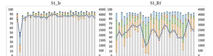
Agronomy 2020, 10, x FOR PEER REVIEW 3 of 17
Agronomy 2020, 10, 984 3 of 16
mean daily maximum and minimum temperatures and mean daily solar radiation of each month
between 1980–2010 in KK. We observed similar values of mean daily maximum and minimum
1980–2010 in KK.and
temperatures We observed
mean dailysimilar
solarvalues of mean
radiation daily
among themaximum and minimum
years. However, temperatures
mean monthly rainfall
andvalues
mean were
daily highly
solar radiation among years.
varied among the years. However,
Textural mean
classes andmonthly
physicalrainfall values were
and chemical highly of
properties
varied
eachamong years.
selected Textural
soil type classesin
are shown and physical
Table and chemical
1. Available properties
water content of each
varies selected
as; S1 > S46 >soil
S44type
(Table
shown in Table 1. Available water content varies as; S1 > S46 > S44 (Table 1).
are1).
40 250
Maximum and minimum temperature (oC)
35
200
30
Solar radiation (MJ/m2)
Rainfall (mm)
25 150
20
15 100
10
50
5
0 0
Jan Feb Mar Apr May Jun Jul Aug Sep Oct Nov Dec
Rain Radn Maxt Mint
Figure
Figure 1. Average
1. Average monthly
monthly climatic
climatic data
data of Khon
of Khon Kaen
Kaen (KK) (KK) between
between 1980–2010;
1980–2010; Rain:
Rain: mean
mean monthly
monthly
rainfall
rainfall (mm);
(mm); Radn:
Radn: mean
mean daily
daily solar
solar radiation
radiation (MJ/m 2
(MJ/m 2 ); Maxt:
); Maxt: mean
mean daily
daily maximum
maximum temperature
temperature
(◦ C);
(°C); Mint:
Mint: mean
mean daily
daily minimum
minimum (◦ C).
temperature
temperature (°C).
Table 1. Physical and chemical properties of selected soil types of KK [4].
Table 1. Physical and chemical properties of selected soil types of KK [4].
Soil Wilting Field Hydraulic Bulk
Soil Soil Texture Wilting Capacity
FieldConductivity
Hydraulic Clay
Bulk Silt Sand
Depth Point Density pH
Soil
Group Texture
Class * % %Clay %
Silt Sand
Depth
(cm) Point (mm/mm)
(mm/mm) Capacity (cm/h) (g/cm3 )
Conductivity Density pH
Group Class * % % %
S1 (cm) Clay soil
0–100 (mm/mm)
0.328 (mm/mm) 0.06
0.461 (cm/h)1.44 (g/cm
68.0 3) 29.0 3 5.4
S44 0–100 Sandy soil 0.038 0.120 13.34 1.7 1 9.5 89.5 5.6
S1
S46
0–100
0–100
Clay soil
Clay loam
0.328
0.133 0.231
0.461 0.36 0.06 1.52 1.44 2968.0 41.8
29.2
29.0 5.1
3 5.4
Sandy
* Soil texture classes
S44 0.038 according0.120
0–100 to the USDA Soil 13.34
textural triangle [29].
1.7 1 9.5 89.5 5.6
soil
Clay
S46 Simulation
2.2. APSIM 0–100 0.133 0.231 0.36 1.52 29.2 29 41.8 5.1
loam
APSIM [30] is a modeling platform
* Soil texture classesthat can beto
according used to simulate
the USDA the performance
Soil textural of a single crop or
triangle [29].
a cropping system under different soil and climatic conditions and permits evaluation of management
2.2. APSIMvia
interventions Simulation
tillage, fertilization, irrigation and selection, timing and crop sequencing (in fixed or
flexible APSIM
rotations) [30][31].
is a For instance,
modeling Ojeda that
platform et al.can
[32]behas
usedused APSIM for
to simulate theforage crop byof
performance considering
a single crop
crop sequences.
or a cropping system under different soil and climatic conditions and permits evaluation of
The APSIM interventions
management 7.10 Sugar model via was usedfertilization,
tillage, for the simulations.
irrigationAPSIM-Sugar
and selection, usestiming
radiation
andusecrop
efficiency (rue) to simulate CDW accumulation by converting intercepted
sequencing (in fixed or flexible rotations) [31]. For instance, Ojeda et al. [32] has used APSIM forradiation into biomass [11].
Onforage
the basis
crop ofby
theconsidering
crop phenological stage, biomass is partitioned among different plant components
crop sequences.
(sucrose,The
leaf,APSIM
structural
7.10stem,
Sugar cabbage
modeland wasroots).
used Itforuses
thesix different crop
simulations. phenologicaluses
APSIM‐Sugar stages to defineuse
radiation
sugarcane growth, i.e., “sowing (from sowing to sprouting), sprouting (from
efficiency (rue) to simulate CDW accumulation by converting intercepted radiation into biomass [11]. sprouting to emergence),
emergence (from
On the basis ofemergence to the beginning
the crop phenological stage,ofbiomass
cane growth), begin cane
is partitioned among (from the beginning
different of cane
plant components
growth to flowering),
(sucrose, flowering
leaf, structural stem,(from flowering
cabbage to the end
and roots). of the
It uses sixcrop) and the
different cropendphenological
of the crop (crop is to
stages
notdefine
currently in the simulated system)” [30]. The model is designed for
sugarcane growth, i.e., “sowing (from sowing to sprouting), sprouting (from sprouting to the simulation of a uniform
cane field usingemergence
emergence), daily time-steps, and predicts
(from emergence tocane yield, cropof
the beginning biomass, sucrosebegin
cane growth), yield, cane
commercial
(from the
sucrose concentration, water use and crop nitrogen uptake on an area basis [33]. Cultivar-specificity,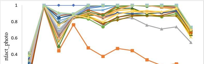
Agronomy 2020, 10, 984                                                                                               4 of 16

plant/ratoon and environmental conditions (climate and soil) are the factors that control this simulation
process [27,33,34].
     CDW of sugarcane plant-crop at harvest was simulated for 30 years (1980–2010) for three
selected soil types under Ir or Rf conditions to study soil and climate interactions on trait parameters.
Management criteria used for the APSIM simulation setup are indicated in Table 2. Planting date was
selected as 28 November of each year in accordance with the previous simulation study [4] to represent
realistic management practices in the region. Soil data (Table 1) and daily weather data for KK from
1980 to 2010 collected by Preecha et al. [4] were used for the simulations.

     Table 2. Management conditions used for the Agricultural Productions System Simulator (APSIM)
     simulations.

                         Criteria                                                 Value
    Planting date                                   November 28
    Crop duration                                   360 days
    Stalk density                                   6.8 stalks/m2
    Planting depth                                  100 mm
    Fertilizer application
                        Fertilization at planting   Urea_N—46.75 kg/ha
        Fertilization at 100 days after planting    Urea_N—46.75 kg/ha
    Water supply by irrigation *
                          Rainfed condition (Rf)    24 mm of irrigation at 7, 14, 21 and 28 days after planting a
                        Irrigation condition (Ir)   24 mm of irrigation with 7 days’ time interval from planting to
                                                    end date of the simulation b
     * The irrigation schedule was manually induced; a to ensuring the crop establishment, b based on the actual
     management practices. The amount of irrigation (24 mm) was assumed with the purpose of avoiding water stress
     and to confirm the difference between Ir and Rf conditions in the simulation. Therefore, Irrigation efficiency is
     considered as one.

2.3. Sensitivity Analysis

2.3.1. Preparation of Training Design Points
      Parameters which control the underlying biophysical process of sugarcane growth in APSIM-Sugar
are categorized into cultivar specific parameters, plant and ratoon class parameters and soil and climate
parameters [11]. Table 3 shows the cultivar-specific parameters implemented in APSIM-Sugar which we
used in this study. Leaf development (leaf size, green_leaf_no, tiller leaf size), phenological development
based on thermal time (tt_emerge_to_begcane, tt_begcane_to_flowering, tt_flowering_to_crop_end) and
partitioning of assimilates (cane_fraction, sucrose_fraction_stalk, stress_factor_stalk, sucrose_delay,
min_sstem_sucrose, min_sstem_sucrose_redn) are controlled by cultivar specific parameters. Parameters
such as green_leaf_no are directly related to express the cultivar traits [11]. Some of the traits are expressed
via a parameter combination. For instance, parameters such as leaf_size and leaf_size_no (position of the
leaf along stalk) together control canopy development [35]. Although, parameters which are related
to later phenological development stages such as tt_begcane_to_flowering and tt_flowering_to_crop_end
included in APSIM-sugar, they remain deactivated until a better physiological basis for prediction
is available [33,35]. Both rue and transp_eff_cf are not considered as cultivar specific parameters in
APSIM-Sugar [11]. However, rue and transp_eff_cf were included in the analysis. In APSIM, dry
matter assimilation is governed by radiation interception and rue in the conditions which soil water
availability is not limited. If the soil water supply is not enough to meet the transpiration demand,
dry matter assimilation is governed by water supply, transp_eff_cf and the vapor pressure deficit.
Moreover, results of SA studies conducted by Sexton et al. [11,35], Gunarathna et al. [27] and Sexton
and Everingham [26] have indicated that both rue and transp_eff_cf may improve simulations based on
cultivar differences.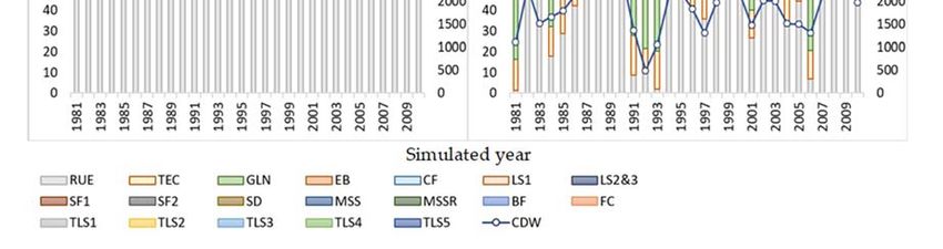
Agronomy 2020, 10, 984                                                                                                5 of 16

                            Table 3. Description of the trait parameters and parameter space [36].

      Parameter Name                    Description                 Level           Code     Units         Range
                                      Leaf area of the         leaf _size_no = 1     LS1      mm2         500–2000
            leaf_size
                                      respective leaf         leaf _size_no = 14    LS2&3     mm2       25,000–70,000
                                                                     and 20
         cane_fraction            Fraction of accumulated                            CF        g/g        0.65–0.80
                                   biomass partitioned to
                                              cane
     sucrose_fraction_stalk       Fraction of accumulated                            SF1       g/g        0.50–0.70
                                   biomass partitioned to
                                            sucrose
       stress_factor_stalk        Stress factor for sucrose                          SF2       n/a         0.2–1.0
                                         accumulation
         sucrose_delay              Sucrose accumulation                             SD       g/m2         0–600
                                              delay
      min_sstem_sucrose           Minimum stem biomass                              MSS       g/m2        450–1500
                                    before partitioning to
                                     sucrose commences
    min_sstem_sucrose_redn        Reduction to minimum                              MSSR      g/m2          0–20
                                     stem sucrose under
                                             stress
     tt_emerg_to_begcane            Accumulated thermal                              EB      ◦C   day    1200–1900
                                  time from emergence to
                                      beginning of cane
    tt_begcane_to_flowering         Accumulated thermal                              BF      ◦C   day    5500–6500
                                  time from beginning of
                                      cane to flowering
    tt_flowering_to_crop_end        Accumulated thermal                              FC      ◦C   day    1750–2250
                                   time from flowering to
                                        end of the crop
         green_leaf_no              Maximum number of                               GLN       No.           9–14
                                    fully expanded green
                                             leaves
                                                              Tiller_leaf_size_no   TLS1    mm2 /mm2        1–6
                                      Tillering factors               =1
        tillerf_leaf_size           according to the leaf     Tiller_leaf_size_no   TLS2    mm2 /mm2        1–6
                                          numbers                     =4
                                                              Tiller_leaf_size_no   TLS3    mm2 /mm2        1–6
                                                                      = 10
                                                              Tiller_leaf_size_no   TLS4    mm2 /mm2        1–6
                                                                      = 16
                                                              Tiller_leaf_size_no   TLS5    mm2 /mm2        1–6
                                                                      = 26
         transp_eff_cf            Transpiration efficiency                          TEC     kg kPa/kg    0.008–0.014
                                        coefficient
              rue                 Radiation use efficiency                          RUE       g/MJ         1.2–2.5

      Initially, 500 parameter combinations were generated based on the parameter ranges indicated in
Table 3 using APSIM package [37] of R software [38]. These training design points were generated as
uniform random numbers distributed between the minimum and maximum values of selected cultivar
trait input parameters (listed in Table 3). Minimum and maximum values of parameters were selected
based on available literature on previous research and APSIM-Sugar documentation (Table 3).
      The ranges for leaf_size, cane_fraction, sucrose_fraction_stalk, stress_factor_stalk, sucrose_delay
min_sstem_sucrose,        min_sstem_sucrose_redn,       tt_emerg_to_begcane,     tt_begcane_to_flowering,
tt_flowering_to_crop_end, green_leaf_no and tillerf_leaf_size were selected based on APSIM-Sugar
documentation [36], Sexton and Everingham [26] and Sexton et al. [11,35].
      According to Sinclair [39], transp_eff_cf ranges between 0.009–0.010 kg kPa/kg for C4 plants like
sugarcane. A recent research conducted by Jackson et al. [40] has reported that under water stressed
conditions, higher transpiration efficiency could be identified for sugarcane cultivars. Therefore, in
order to represent the response of sugarcane to water stressed conditions, the present study has used
the range of transp_eff_cf as 0.008–0.014 kg kPa/kg following Gunarathna et al. [27].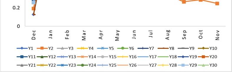
Agronomy 2020, 10, 984                                                                                  6 of 16

     In the APSIM-Sugar model, rue parameter is fixed as 1.8 g/MJ for plant crops and 1.65 g/MJ
for ratoon crops [36]. It is reported that a considerable variation in rue could be occurred due to
temperature variations, soil water deficit or excess [33], crop class and age, lodging, soil fertility
(Nitrogen deficit) and culm death [41]. Considering the intercepted photosynthetically active radiation,
Ferreira et al. [42] have found that rue of sugarcane in single and combined spacing as 2.73 (±0.09) and
2.78 (±0.25) g/MJ, respectively. Further, Olivier et al. [43] have reported rue value of 1.75 g/MJ for N19
sugarcane variety. Meki et al. [44] have obtained rue value of 2.06 g/MJ for their study on modeling of
specific crop parameter attributes of two-year sugarcane growth cycle. Hence, by considering values
of previous studies, we have used 1.2–2.5 g/MJ as the range for rue.
     Above mentioned parameter combinations were then simulated in APSIM-Sugar for 30 years
under three selected soil types and Ir or Rf conditions (described in Section 2.2). APSIM output values
(CDW) corresponding to each parameter combination and environmental and management condition
(180 APSIM output files and each file including 500 outputs) were obtained from the simulations.
Both parameter combination files and corresponding APSIM output files were used as training design
points for emulator generation and validation during the GSA.

2.3.2. Gaussian-Process-Based Global Sensitivity Analysis
      To conduct SA for complex simulation models, an increasing number of studies have focused on
model emulation. According to Villa-Vialaneix et al. [45], it is a common approach to use GP when
generating emulators [20,46], even though other options are available as well. GP can be defined as a
distribution for a function. According to O’Hagan et al. [46], each value of a function has a normal
distribution, and a set of function values has a multivariate normal distribution. Therefore, GPs and the
normal distribution both have equal mathematically convenient properties. During emulator building,
the original model is described by assigning a GP prior, and then the prior is updated using a series of
model runs by applying the Bayes theorem. The emulator is the resulting posterior distribution [47].
      SA was conducted by using GP-based emulation implemented in the Gaussian emulation machine
for sensitivity analysis (GEM-SA) software package [47]. A more detailed description of the mathematics
underlying GEM-SA can be found in Kennedy and O’Hagan [7] and Oakley and O’Hagan [22].
The GEM-SA package calculates two variance-based sensitivity indices, the main-effect index (Si ) and
the total-effect index (STi ).
      Equation (1) defines the main-effect index as:
                                                   n              o
                                                Var E( f (X) xi )
                                           Si =                                                           (1)
                                                  Var f (X)

where “Var{f (X)} is the total variance in the output given variations of all parameters and Var{E(f (X)|xi )}
is the variance in the expected output of f (X) given xi . Therefore, Si represents the expected reduction
in output variance if parameter xi is known” [22].
      Equation (2) defines the total-effect index as:
                                                     n              o
                                                  Var E( f (X) xi )
                                        TSi = 1 −                                                         (2)
                                                    Var f (X)

where “Var{E(f (X)|xi )} is the variance in the expected output of f (X) if all parameters except xi are known.
Therefore, TSi represents the total effect of the parameter xi and all its interactions. If parameters are
linearly additive (i.e., no strong interactions), Si and STi should be equal” [22].
     Prepared training design points for the outputs of the APSIM-Sugar and the parameter
combinations (described in Section 2.3.1) were run in GEM-SA. 300 training points of APSIM outputs
and corresponding parameter combinations were used to generate emulators. 180 emulators (30 × 3 × 2)
for combinations of each year (30), each soil type (3) and Ir or Rf condition were generated. While
developing the emulators, remaining 200 parameter combinations were used in GEM-SA to obtain
Agronomy 2020, 10, 984 7 of 16
emulator predictions (emulator predicted CDW). These predictions were graphed with remaining
APSIM-output training design points and coefficient of determination (R2 ) were calculated to evaluate
how well emulator can predict the APSIM simulator outputs. R2 range between 1 to 0 and emulators
with higher accuracy can be identified with R2 values close to one.
When running the GEM-SA, linear term for each input was set as the prior mean option for the
outputs, as it allows us to observe the output trend in response to input changes. Leave-one-out
cross-validation was selected to evaluate the accuracy of emulators built by GEM-SA. GEM-SA
calculated Si and TSi values for each parameter corresponding to each emulator were recorded. Further,
GEM-SA calculates leave-one-out cross-validated RMSSE (Equation (3)) and sigma-squared value (σ2 )
for each emulator [48]; these values were used to represent the performance of model emulators with
reference to environmental and management conditions in addition to R2 .
Equation (3) defines cross-validated RMSSE as:
s
− ŷ)/si )2
Pn
i=1 (( yi
C VRMSSE = (3)
n
where, “yi is the true output for the ith training run, ŷ is the corresponding emulator approximation,
si is the standard deviation calculated with the ith training point removed and n is the number of
runs” [48].
The cross-validated RMSSE is close to 1 if the actual error variance is accurately estimated by the
emulator variance [49], while lower and higher values indicate overestimation and underestimation,
respectively [50].
The σ2 value is an effective measure that indicates an emulator’s non-linearity by expressing
emulator variance after output standardization [51]. The values of σ2 ranges near 0 for a linear model
and has greater values (without a defined cutoff value) for moderately to highly nonlinear models [49].
The sensitivity of the model outputs to cultivar parameters was explored using stacked column
bar chart with Si indices. Parameters with the strongest effects on simulated CDW were identified from
Si values and were further examined with reference to environmental and management conditions in
KK by using main effect plots.
3. Results and Discussion
3.1. Emulator Accuracy
R2 calculated by using the APSIM simulated CDW and emulator predicted CDW, and GEM-SA
internally calculated σ2 and cross-validated RMSSE values were used to evaluate the performances
of generated emulators. Scatter plots of Figure 2 indicate the linear relationship between the APSIM
simulated CDW and emulator predicted CDW. As it is complicated to show all the graphs, here we
present only some examples to represent all the conditions. However, calculated R2 for all conditions
were ranged between 0.85 to 0.99 and closer to one indicating that all emulators can successfully
approximate the APSIM simulators.
The calculated σ2 values of all emulators ranged between 0.08 and 0.89 (Figure 3a).
Petropoulos et al. [51] obtained σ2 values ranging from 0.13 to 1.6 for their emulators and concluded
that their parameters deviated only moderately from linearity. Gunarathna et al. [27] obtained
σ2 values ranging from 0.10 to 1.43 and concluded that their models showed good to moderate
linearity. Hence, we can conclude that our emulators showed good linearity in each environmental
and management condition.internally calculated σ2 and cross-validated RMSSE values were used to evaluate the performances of
generated emulators. Scatter plots of Figure 2 indicate the linear relationship between the APSIM
simulated CDW and emulator predicted CDW. As it is complicated to show all the graphs, here we
present only some examples to represent all the conditions. However, calculated R2 for all conditions
were ranged
Agronomy between
2020, 10, 984 0.85 to 0.99 and closer to one indicating that all emulators can successfully
8 of 16
approximate the APSIM simulators.
S1_Ir_Y 10 S1_Ir_Y 20 S1_Rf _Y 10 S1_Rf _Y 20
6000
4000
Emulator predicted sugarcane dry weight (g/m )
2
2000
2 2 2 2
R = 0.96 R = 0.98 R = 0.99 R = 0.99
0
S44_Ir_Y 10 S44_Ir_Y 20 S44_Rf _Y 10 S44_Rf _Y 20
6000
4000
2000
2 2 2 2
R = 0.99 R = 0.99 R = 0.99 R = 0.99
0
S46_Ir_Y 10 S46_Ir_Y 20 S46_Rf _Y 10 S46_Rf _Y 20
6000
4000
2000
2 2 2 2
R = 0.99 R = 0.99 R = 0.99 R = 0.98
0
2000
4000
6000
2000
4000
6000
2000
4000
6000
2000
4000
6000
0
0
0
0
2
APSIM simulated sugarcane dry weight (g/m )
Figure 2. Relationship
Figure 2. Relationship between APSIM simulated cane dry weight weight (CDW)
(CDW) and and emulator
emulator predicted
predicted
CDW
CDW of of year
year (Y)
(Y) 10
10 and
and year
year (Y)
(Y) 20
20 between
between (1980–2010)
(1980–2010) under
under three
three soil
soil types
types (S1,
(S1, S44
S44 and
and S46)
S46) and
and
irrigated
irrigated (Ir)
(Ir) and
and rainfed
rainfed
Agronomy 2020, 10, x FOR PEER REVIEW(Rf)
(Rf) conditions.
conditions. Solid red lines indicate linear fit to
to the
the APSIM
APSIM simulated
simulated 9 of 17
CDW
CDW andand emulator
emulator predicted
predicted CDW
CDW values.
values.
The 1.4
1.00calculated σ2 values of all emulators ranged between 0.08 and 0.89 (Figure 3a). Petropoulos
et al. [51] obtained σ values ranging from 0.13 to 1.6 for their emulators and concluded that their
2
Cross‐Validated RMSSE values
parameters deviated only moderately from linearity. Gunarathna et al. [27] obtained σ2 values
0.75
Sigma‐squired values
ranging from 0.10 to 1.43 and concluded that their models 1.2 showed good to moderate linearity. Hence,
we can conclude that our emulators showed good linearity in each environmental and management
condition.
0.50
1.0
0.25
0.8
0.00
Rf
Rf
Ir
Ir
f
f
f
_Ir
Ir
Ir
_R
f
R
R
_I r
4_
6_
_R
4_
6_
4_
6_
4_
6_
S1
S1
S4
S4
S1
S4
S4
S1
S4
S4
S4
S4
(a) (b)
Box plots of (a) σ22 and
Figure 3. Box and (b) cross‐validated
cross-validated root‐mean‐squared
root-mean-squared standardized
standardized error
error (RMSSE)
(RMSSE)
values of the emulator
emulator build
build for
for three
three soil
soil types
types (S1,
(S1, S44
S44 and
and S46)
S46) and
and irrigated
irrigated (Ir)
(Ir) and
and rainfed
rainfed (Rf)
(Rf)
The thick
condition: The thick black
black lines
lines indicate
indicate the
the median,
median, the
the boxes
boxes indicate
indicate the
the interquartile
interquartile range
range (IQR),
(IQR),
the whiskers
whiskers indicate
indicate1.5
1.5times
timesthetheIQR
IQRand
andthethe
black points
black indicate
points outliers
indicate beyond
outliers 1.5 times
beyond the IQR.
1.5 times the
IQR.
Computed cross-validated RMSSE values of emulators ranged between 0.82 and 1.21 (Figure 3b).
These values were
Computed lower than the
cross‐validated valuesvalues
RMSSE reported by Kennedy
of emulators et al. [47]
ranged and Petropoulos
between et (Figure
0.82 and 1.21 al. [51],
3b). These values were lower than the values reported by Kennedy et al. [47] and Petropoulos et al.
[51], and were close to one in all the SA experiments, suggesting that the true model can be well
represented by the generated emulators.
3.2. Determination of Parameter SensitivityAgronomy 2020, 10, 984 9 of 16
and were close to one in all the SA experiments, suggesting that the true model can be well represented
by the generated emulators.
3.2. Determination of Parameter Sensitivity
Studying the sensitivity of model outputs to cultivar parameters under different environmental
and management conditions would help to improve the calibration efficiency of the model. Moreover,
when determining the appropriate management practices for sugarcane cultivation, it is important to
consider parameters that strongly affect sugarcane yield. Therefore, to determine parameter sensitivity
across environmental and management conditions, we examined Si and STi computed by GEM-SA.
However, we disregard the STi values because of the observation of less difference among Si and STi
values and a greater fraction of variability being explained by Si . The Si values of each parameter for
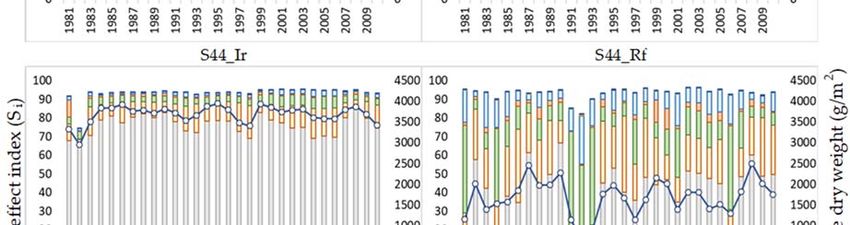
all simulated conditions are shown in Figure 4. In order to explain the differences of Si among each
condition APSIM simulated CDW was included (Figure 4).
Agronomy 2020, 10, x FOR PEER REVIEW 10 of 17
Figure
Figure ParameterSSi ivalues
4.4.Parameter values and CDW of
of soil
soiltype
typeS1,
S1,S44
S44and
andS46,
S46,under
underIr Ir
andand
Rf Rf conditions
conditions across
across
3030
simulated
simulatedyears
yearsfrom
from1980–2010.
1980–2010.
Based on the Si values of 30 years of each soil type under Ir or Rf conditions, rue (RUE),
green_leaf_no (GLN), transp_eff_cf (TEC), tt_emerg_to_begcane (EB) and cane_fraction (CF) were
identified as the most influential parameters on CDW (these parameters together explained >90% of
the variability of CDW) while, TLS5, LS2 and 3, TLS4, SF1, BF, MSSR, MSS, FC, SD, TLS2, TLS1, TLS3,
LS1, SF2 were identified as the insensitive parameters (each parameter explainedAgronomy 2020, 10, 984 10 of 16
Based on the Si values of 30 years of each soil type under Ir or Rf conditions, rue (RUE), green_leaf_no
(GLN), transp_eff_cf (TEC), tt_emerg_to_begcane (EB) and cane_fraction (CF) were identified as the most
influential parameters on CDW (these parameters together explained >90% of the variability of CDW)
while, TLS5, LS2 and 3, TLS4, SF1, BF, MSSR, MSS, FC, SD, TLS2, TLS1, TLS3, LS1, SF2 were identified
as the insensitive parameters (each parameter explained > S46
sand 3%) S46 (clay
(clay 29.2%,
29.2%, silt
silt 29%,
29%, sand
sand
41.8%) > S44 (clay 1%, silt 9.5%, sand 89.5%) (Table 1). As indicated in Figure 4 this will largely
41.8%) > S44 (clay 1%, silt 9.5%, sand 89.5%) (Table 1). As indicated in Figure 4 this will largely reduce reduce
the CDW and therefore it is crucial to manage nitrogen application when molding higher rainfall
periods to reduce the nitrogen stress specially in S1 soil type.
It is observed that sensitivity of RUE reduced with available water content. Sensitivity of RUE
became lower in Rf condition than in Ir condition (Figure 4). Under Rf, sensitivity of RUE was the
highest in S1 and weakened in S46 and S44 soils. This is because the available soil water content inAgronomy 2020, 10, 984 11 of 16
the CDW and therefore it is crucial to manage nitrogen application when molding higher rainfall
periods to reduce the nitrogen stress specially in S1 soil type.
It is observed that sensitivity of RUE reduced with available water content. Sensitivity of RUE
became lower in Rf condition than in Ir condition (Figure 4). Under Rf, sensitivity of RUE was the
highest in S1 and weakened in S46 and S44 soils. This is because the available soil water content in
selected soil types are varied; S1 > S46 > S44 (Table 1). This was more evident in years which represent
lower annual rainfall (year: 1981, 1984, 1991, 1992, 1993 and 2006 in Figure 4) than the other years
during the study period.
For CDW, TEC was the second most influential parameter under each environmental and
management condition in KK based on average S1 values across study period. However, the sensitivity
of TEC is higher in Rf than Ir (Figure 4) indicating that TEC is highly sensitive to water stressed
conditions. Sexton and Everingham [26] has also found similar results for their study. This is because
in APSIM, dry matter assimilation is governed by radiation interception and RUE in the conditions
which soil water availability is not limited. However, in case the soil water supply is not enough to
meet the transpiration demand, dry matter assimilation is governed by water supply, TEC and the
vapor pressure deficit.
GLN is highly influential under water stressed conditions. GLN indicated higher Si under Rf than
Ir. Although GLN was the third most influential parameter based on the average Si values, it became
the second most influential one in the year of 1981, 1984, 1991, 1992, 1993 and 2006 (Figure 4). These
years indicated lower rainfall compared to other years and under Rf condition water stress becomes
more sever. Higher water stresses may create leaf emergence rate reduction and leaf senescence rate
increment, causing significant reduction in GLN and reduce CDW [53]. This was more evident in our
results of year 1991, 1992 and 1993 (the years with lowest rainfall) (Figure 4) under S44 (soil type with
lowest water availability) and Rf.
For CDW, CF was the fourth most influential parameter and EB was the fifth most influential
parameter. Both indicated higher Si values for Rf than Ir indicating high sensitivity for water stresses
(Figure 4). In addition, they indicated high sensitivity for year 1982 under S1 and Ir which we previously
identified as nitrogen stressed condition. This is not surprisingly because in APSIM, water deficit and
nitrogen deficit both cause for limiting the biomass partitioning in the stem (CF) and phenological
development based on thermal time (EB).
Computed Si indicated that sensitivity of RUE, GLN, TEC, EB and CF explains more than 90% of
total variance for most of the simulator outputs across all simulated years, while other parameters had
much weaker effects (Figure 4). Similar studies on cultivar-by-environment interactions conducted
by Sexton et al. [11] and Gunarathna et al. [27] also found these parameters among highly influential
parameters under their selected environmental and management conditions. Therefore, when modeling
CDW using APSIM-Sugar those influential parameters can be used to calibrate the model. When
such calibrations are streamlined, non-influential (low Si ) parameters could be fixed to default values.
Parameters such as RUE and TEC are ideal for statistical calibration of APSIM-Sugar as they are
difficult in measuring. By measuring comparatively simple-to-obtain parameters like GLN, it can be
reduced the number of parameters used for calibration.
3.3. Sensitivity of Highly Influential Parameters
Knowledge of sensitive parameters is needed for the improvement of simulations of sugarcane
growth under various environmental and management conditions. Therefore, we further analyzed the
response of outputs to selected environmental and management conditions. The response of CDW to
the highly influential parameters (CF, EB, GLN, TEC and RUE) was visualized by plotting the mean of
the emulator’s main effects from 6000 randomly selected iterations (Figure 6).Agronomy 2020, 10, 984 12 of 16
Agronomy 2020, 10, x FOR PEER REVIEW 13 of 17
Figure 6.
Figure Parameter main effect
6. Parameter effectof
ofhighly
highlyinfluential
influentialparameters
parametersunder soilsoil
under types (S1,(S1,
types S44S44
andand
S46),S46),
and
Ir (blue)
and and and
Ir (blue) Rf (orange) conditions
Rf (orange) for CDW.
conditions for CDW.
Statistical calibration
Statistical calibration ofof RUE
RUE and and TECTEC parameters
parameters wouldwould improve
improve the the simulation
simulation of of cultivar
cultivar
differences in CDW. When parameter value of RUE increased from
differences in CDW. When parameter value of RUE increased from 1.2 g/MJ to 2.5 g/MJ we could 1.2 g/MJ to 2.5 g/MJ we could
observe high
observe high increment
increment in in CDW
CDW (Figure
(Figure 6).6). This
This relationship
relationshipwas was stronger
stronger in in Ir
Ir condition
condition when
when
compared with Rf condition and the strongest in soil types with the highest
compared with Rf condition and the strongest in soil types with the highest available water content available water content
(S1, S46)
(S1, S46) and
and weakened
weakened withwith the
the lowest
lowest available
available water
water content (S1 >
content (S1 S46 >>S44).
> S46 S44).These
Theseresults
resultsconfirm
confirm
thatCDW
that CDWisishighly
highlysensitive
sensitivetotoRUE,RUE, which
which is directly
is directly connected
connected with
with thethe availability
availability of moisture
of moisture for
for plants. In addition, when increasing the TEC parameter value from
plants. In addition, when increasing the TEC parameter value from 0.008–0.014 kg kPa/kg, CDW 0.008–0.014 kg kPa/kg, CDW
tendsto
tends toincrease
increaseslightly
slightlyininall
allconditions,
conditions,however
howeverthis thiswas
was more
more evident
evident in in
RfRf conditions
conditions than
than in
in Ir
Ir conditions (Figure 6). In APSIM, both RUE and TEC do not differ
conditions (Figure 6). In APSIM, both RUE and TEC do not differ by default [36,54]. Therefore, by default [36,54]. Therefore,
statistical calibration
statistical calibration of of highly
highly influential
influential RUE RUE andand TECTEC parameters
parameters are are crucial
crucial to to achieve
achieve higher
higher
accuracy when
accuracy when modeling
modeling thethe CDW
CDW in in KK.
KK.
Cultivars with higher GLN
Cultivars with higher GLN and lower CFand lower CF values
valueswill
will be
be more
more beneficial
beneficial whenwhen modeling
modeling CDWCDW
under any of the environmental and management conditions in KK. This
under any of the environmental and management conditions in KK. This is because under all is because under all simulated
conditions,conditions,
simulated the influencetheofinfluence
GLN on of CDWGLN shows
on CDWan increasing
shows antrend while CF
increasing trendindicting
while CFthe indicting
declining
trend when increasing the parameter values from 9 to 14 and 0.65 to 0.8 g/g,
the declining trend when increasing the parameter values from 9 to 14 and 0.65 to 0.8 g/g, respectively respectively (Figure 6).
However, ◦
(Figure 6).itHowever,
seems thatitincreasing
seems that the parameterthe
increasing value from 1200
parameter to 1900
value fromC1200day of to EB
1900may°Ccause
day oflower
EB
increment in CDW compared to other parameters (Figure 6). These results
may cause lower increment in CDW compared to other parameters (Figure 6). These results are very are very important when
parameterizing
important whenthe crop model forthe
parameterizing KKcropbecause
model theyforareKK
useful in reducing
because they are theuseful
number in of parameters
reducing the
to be calibrated
number and avoiding
of parameters over-parameterization.
to be calibrated and avoiding over‐parameterization.
We could study the sensitivity of model outputs to cultivar parameters under different
environmental conditions of tropical sugarcane production in KK, Thailand. Determination ofAgronomy 2020, 10, 984 13 of 16
We could study the sensitivity of model outputs to cultivar parameters under different
environmental conditions of tropical sugarcane production in KK, Thailand. Determination of
variability in the influence of model input parameters on model output could have a considerable
impact on studies of cultivar-by-environment interactions. Such studies would improve the efficiency
and accuracy of crop modeling, which is computationally expensive, and will be ultimately important
for identification of appropriate management strategies to cope with both temporal and spatial
variability of crop yield. Therefore, we encourage future research focused on a range of soil types,
climate interactions and different water regimes.
4. Conclusions
Our study focused on the use of GP-based emulators to analyze parameter sensitivity in the
APSIM-Sugar model under different environmental and management conditions in KK, Thailand.
The emulators we obtained, which corresponded to each environmental and management condition
across simulated years showed satisfactory results, as evidenced by R2 , σ2 and cross-validated RMSSE
values, indicate that these emulators can successfully replace the simulators. rue (RUE), green_leaf_no
(GLN), transp_eff_cf (TEC), tt_emerg_to_begcane (EB) and cane_fraction (CF) were the most influential
parameters regardless of soil type, Ir or Rf conditions. Other analyzed parameters had little influence
on the simulator output. Outcomes of our study are beneficial in enhancing the efficiency and accuracy
of crop modeling. Further, findings can be used to identify appropriate management strategies to
address temporal and spatial variability of sugarcane yield in KK.
Author Contributions: Conceptualization, methodology and formal analysis, W.B.M.A.C.B and K.S.; investigation
and writing—Original draft preparation, W.B.M.A.C.B; writing—Review and editing, W.B.M.A.C.B and R.H.K.R.;
supervision, K.S., P.K. and T.N. All authors have read and agreed to the published version of the manuscript.
Funding: This research received no external funding.
Conflicts of Interest: The authors declare no conflict of interest.
References
1. Manivong, P.; Bourgois, E. White Paper: Thai Sugarcane Sector and Sustainability; FairAgora Asia Co. Ltd.:
Bangkok, Thailand, 2017.
2. Hongthong, P.; Patanothai, A. Variations in Sugarcane Yield among Farmers’ Fields and Their Causal Factors
in Northeast Thailand. Int. J. Plant Prod. 2017, 11, 533–548. [CrossRef]
3. Rambo, A.T. The Agrarian Transformation in Northeastern Thailand: A Review of Recent Research. Southeast
Asian Stud. 2017, 6, 211–245. [CrossRef]
4. Preecha, K.; Sakai, K.; Pisanjaroen, K.; Sansayawichai, T.; Cho, T.; Nakamura, S.; Nakandakari, T. Calibration
and Validation of Two Crop Models for Estimating Sugarcane Yield in Northeast Thailand. Trop. Agric. Dev.
2016, 60, 31–39. [CrossRef]
5. Jeuffroy, M.H.; Barbottin, A.; Jones, J.W.; Lecoeur, J. Crop Models with Genotype Parameters. In Working with
Crop Models, 1st ed.; Wallach, D., Makowski, D., Jones, J.W., Eds.; Elsevier: Amsterdam, The Netherlands,
2006; pp. 281–308.
6. Ojeda, J.J.; Rezaei, E.E.; Remenyi, T.A.; Webb, M.A.; Webber, H.A.; Kamali, B.; Harris, R.M.B.; Brown, J.N.;
Kidd, D.B.; Mohammed, C.L.; et al. Effects of Soil and Climate Data Aggregation on Simulated Potato Yield
and Irrigation Water Requirement. Sci. Total Environ. 2020, 710, 135589. [CrossRef]
7. Kennedy, M.C.; O’Hagan, A. Bayesian Calibration of Computer Models. J. R. Stat. Soc. Ser. B (Stat. Methodol.)
2001, 63, 425–464. [CrossRef]
8. Song, X.; Zhan, C.; Kong, F.; Xia, J. Advances in the Study of Uncertainty Quantification of Large-Scale
Hydrological Modeling System. J. Geogr. Sci. 2011, 21, 801–819. [CrossRef]
9. Ewert, F.; van Ittersum, M.K.; Heckelei, T.; Therond, O.; Bezlepkina, I.; Andersen, E. Scale Changes and
Model Linking Methods for Integrated Assessment of Agri-Environmental Systems. Agric. Ecosyst. Environ.
2011, 142, 6–17. [CrossRef]Agronomy 2020, 10, 984 14 of 16
10. Song, X.M.; Kong, F.Z.; Zhan, C.S.; Han, J.W.; Zhang, X.H. Parameter Identification and Global Sensitivity
Analysis of Xin’anjiang Model Using Meta-Modeling Approach. Water Sci. Eng. 2013, 6, 1–17. [CrossRef]
11. Sexton, J.; Everingham, Y.L.; Inman-Bamber, G. A Global Sensitivity Analysis of Cultivar Trait Parameters
in a Sugarcane Growth Model for Contrasting Production Environments in Queensland, Australia. Eur. J.
Agron. 2017, 88, 96–105. [CrossRef]
12. Muñoz-Carpena, R.; Zajac, Z.; Kuo, Y.M. Global Sensitivity and Uncertainty Analyses of the Water Quality
Model VFSMOD-W. Trans. ASABE 2007, 50, 1719–1732. [CrossRef]
13. Cukier, R.I.; Fortuin, C.M.; Shuler, K.E.; Petschek, A.G.; Schaibly, J.H. Study of the Sensitivity of Coupled
Reaction Systems to Uncertainties in Rate Coefficients. I Theory. J. Chem. Phys. 1973, 59, 3873–3878.
[CrossRef]
14. Mara, T.A.; Tarantola, S. Application of Global Sensitivity Analysis of Model Output to Building Thermal
Simulations. Build. Simul. 2008, 1, 290–302. [CrossRef]
15. Saltelli, A. Making Best Use of Model Evaluations to Compute Sensitivity Indices. Comput. Phys. Commun.
2002, 145, 280–297. [CrossRef]
16. Homma, T.; Saltelli, A. Importance Measures in Global Sensitivity Analysis of Nonlinear Models. Reliab. Eng.
Syst. Saf. 1996, 52, 1–17. [CrossRef]
17. Sobol’, I.M. On Sensitivity Estimation for Nonlinear Mathematical Models. Matem. Mod. 1990, 2, 112–118.
18. Saltelli, A.; Chan, K.; Scott, M. Sensitivity Analysis; Probability and Statistics Series; John Wiley Sons:
Chichester, UK, 2000.
19. Specka, X.; Nendel, C.; Wieland, R. Temporal Sensitivity Analysis of the MONICA Model: Application of
Two Global Approaches to Analyze the Dynamics of Parameter Sensitivity. Agriculture 2019, 9, 37. [CrossRef]
20. O’Hagan, A. Bayesian Analysis of Computer Code Outputs: A Tutorial. Reliab. Eng. Syst. Saf. 2006, 91,
1290–1300. [CrossRef]
21. Sacks, J.; Welch, W.J.; Mitchell, T.J.; Wynn, H.P. Design and Analysis of Computer Experiments. Stat. Sci.
1989, 4, 409–423. [CrossRef]
22. Oakley, J.E.; O’Hagan, A. Probabilistic Sensitivity Analysis of Complex Models: A Bayesian Approach. J. R.
Stat. Soc. Ser. B Stat. Methodol. 2004, 66, 751–769. [CrossRef]
23. Uusitalo, L.; Lehikoinen, A.; Helle, I.; Myrberg, K. An Overview of Methods to Evaluate Uncertainty of
Deterministic Models in Decision Support. Environ. Model. Softw. 2015, 63, 24–31. [CrossRef]
24. Boukouvalas, A.; Cornford, D.; Maniyar, D.; Singer, A. Gaussian Process Emulation of Stochastic Models:
Developments and Application to Rabies Modelling. In Proceedings of the RSS 2008 Conference, Nottingham,
UK, 1–5 September 2008.
25. Rasmussen, C.E.; Williams, C.K.I. Gaussian Processes for Machine Learning Cambridge; MIT Press: Cambridge,
MA, USA, 2006.
26. Sexton, J.; Everingham, Y. Global Sensitivity Analysis of Key Parameters in A Process-Based Sugarcane
Growth Model—A Bayesian Approach. In Proceedings of the 7th International Congress on Environmental
Modelling and Software, San Diego, CA, USA, 15–19 June 2014.
27. Gunarathna, M.H.J.P.; Sakai, K.; Nakandakari, T.; Momii, K.; Kumari, M.K.N. Sensitivity Analysis of Plant
and Cultivar-Specific Parameters of APSIM-Sugar Model: Variation between Climates and Management
Conditions. Agronomy 2019, 9, 242. [CrossRef]
28. Khon Kaen Climate. Available online: https://en.climate-data.org/asia/thailand/khon-kaen-province/khon-
kaen-4291/ (accessed on 19 November 2019).
29. USDA. Soil Texture Calculator. Available online: https://www.nrcs.usda.gov (accessed on 15 November 2019).
30. Holzworth, D.P.; Huth, N.I.; de Voil, P.G.; Zurcher, E.J.; Herrmann, N.I.; McLean, G.; Chenu, K.;
van Oosterom, E.J.; Snow, V.; Murphy, C.; et al. APSIM–evolution towards a new generation of agricultural
systems simulation. Environ. Model. Softw. 2014, 62, 327–350. [CrossRef]
31. Wang, E.; Robertson, M.J.; Hammer, G.L.; Carberry, P.S.; Holzworth, D.; Meinke, H.; Chapman, S.C.;
Hargreaves, J.N.G.; Huth, N.I.; McLean, G. Development of a Generic Crop Model Template in the Cropping
System Model APSIM. Eur. J. Agron. 2002, 18, 121–140. [CrossRef]
32. Ojeda, J.J.; Pembleton, K.G.; Caviglia, O.P.; Islam, M.R.; Agnusdei, M.G.; Garcia, S.C. Modelling Forage Yield
and Water Productivity of Continuous Crop Sequences in the Argentinian Pampas. Eur. J. Agron. 2018, 92,
84–96. [CrossRef]Agronomy 2020, 10, 984 15 of 16
33. Keating, B.A.; Robertson, M.J.; Muchow, R.C.; Huth, N.I. Modelling sugarcane production systems. I.
Description and validation of the sugarcane module. F. Crop. Res. 1999, 61, 253–271. [CrossRef]
34. Dias, H.B.; Inman-Bamber, G.; Bermejo, R.; Sentelhas, P.C.; Christodoulou, D. New APSIM-Sugar Features
and Parameters Required to Account for High Sugarcane Yields in Tropical Environments. F. Crop. Res. 2019,
235, 38–53. [CrossRef]
35. Sexton, J.; Everingham, Y.; Inman-Bamber, G. A Theoretical and Real-World Evaluation of Two Bayesian
Techniques for the Calibration of Variety Parameters in a Sugarcane Crop Model. Environ. Model. Softw.
2016, 83, 126–142. [CrossRef]
36. Keating, B. The APSIM Sugar Model. Available online: http://apsrunet.apsim.info/svn/development/trunk/
apsim/sugar/docs/sugar_pseudo.html#sugar_dm_partition_pot (accessed on 23 November 2019).
37. Stanfill, B. Apsimr: Edit, Run and Evaluate APSIM Simulations Easily Using R. Available online:
https://cran.r-project.org/web/packages/apsimr/index.html (accessed on 23 November 2019).
38. R Core Team. R: A Language and Environment for Statistical Computing; R Foundation for Statistical Computing:
Vienna, Austria. Available online: https://www.R-project.org/ (accessed on 25 November 2019).
39. Sinclair, T.R. Is Transpiration Efficiency a Viable Plant Trait in Breeding for Crop Improvement?
Funct. Plant Biol. 2012, 39, 359–365. [CrossRef]
40. Jackson, P.A.; Basnayake, J.; Inman-Bamber, G.; Lakshmanan, P. Selecting Sugarcane Varieties with Higher
Transpiration Efficiency. In Proceedings of the Australian Society of Sugar Cane Technologists, Broadbeach,
Australia, 28 April–1 May 2014; Volume 36.
41. Park, S.E.; Robertson, M.; Inman-Bamber, N.G. Decline in the Growth of a Sugarcane Crop with Age under
High Input Conditions. F. Crop. Res. 2005, 92, 305–320. [CrossRef]
42. Ferreira, R.A.; de Souza, J.L.; Lyra, G.B.; Escobedo, J.F.; Santos, M.V.C. Energy Conversion Efficiency in
Sugarcane under Two Row Spacings in Northeast of Brazil. Rev. Bras. Eng. Agrícola e Ambient. 2015, 19,
741–747. [CrossRef]
43. Olivier, F.C.; Singels, A.; Eksteen, A.B. Water and Radiation Use Efficiency of Sugarcane for Bioethanol
Production in South Africa, Benchmarked against Other Selected Crops. S. Afr. J. Plant Soil 2016, 33, 1–11.
[CrossRef]
44. Meki, M.N.; Kiniry, J.R.; Youkhana, A.H.; Crow, S.E.; Ogoshi, R.M.; Nakahata, M.H.; Tirado-Corbalá, R.;
Anderson, R.G.; Osorio, J.; Jeong, J. Two-Year Growth Cycle Sugarcane Crop Parameter Attributes and Their
Application in Modeling. Agron. J. 2015, 107, 1310–1320. [CrossRef]
45. Villa-Vialaneix, N.; Follador, M.; Ratto, M.; Leip, A. A Comparison of Eight Metamodeling Techniques for
the Simulation of N2 O Fluxes and N Leaching from Corn Crops. Environ. Model. Softw. 2012, 34, 51–66.
[CrossRef]
46. O’Hagan, A. Probabilistic Uncertainty Specification: Overview, Elaboration Techniques and Their Application
to a Mechanistic Model of Carbon Flux. Environ. Model. Softw. 2012, 36, 35–48. [CrossRef]
47. Kennedy, M.C.; Anderson, C.W.; Conti, S.; O’Hagan, A. Case Studies in Gaussian Process Modelling of
Computer Codes. Reliab. Eng. Syst. Saf. 2006, 91, 1301–1309. [CrossRef]
48. Kennedy, M.C.; Petropoulos, G.P. GEM-SA: The Gaussian Emulation Machine for Sensitivity Analysis.
In Sensitivity Analysis in Earth Observation Modelling; George, P.P., Prashant, K.S., Eds.; Elsevier: Amsterdam,
The Netherlands, 2017; pp. 341–361. ISBN 978-0-12-803011-0.
49. Qin, X.; Wang, H.; Li, Y.; Li, Y.; McConkey, B.; Lemke, R.; Li, C.; Brandt, K.; Gao, Q.; Wan, Y.; et al. A Long-Term
Sensitivity Analysis of the Denitrification and Decomposition Model. Environ. Model. Softw. 2013, 43, 26–36.
[CrossRef]
50. Sexton, J. Bayesian Statistical Calibration of Variety Parameters in Asugarcane Crop Model. Master’s Thesis,
James Cook University, Townsville, Australia, April 2015.
51. Petropoulos, G.; Wooster, M.J.; Carlson, T.N.; Kennedy, M.C.; Scholze, M. A Global Bayesian Sensitivity
Analysis of the 1d SimSphere Soil-Vegetation-Atmospheric Transfer (SVAT) Model Using Gaussian Model
Emulation. Ecol. Modell. 2009, 220, 2427–2440. [CrossRef]
52. Ojeda, J.J.; Volenec, J.J.; Brouder, S.M.; Caviglia, O.P.; Agnusdei, M.G. Evaluation of Agricultural Production
Systems Simulator as Yield Predictor of Panicum Virgatum and Miscanthus x Giganteus in Several US
Environments. GCB Bioenergy 2017, 9, 796–816. [CrossRef]Agronomy 2020, 10, 984 16 of 16
53. Smit, M.A.; Singels, A.; van Antwerpen, A. Differences in Canopy Development of Two Sugarcane Cultivars
under Conditions of Water Stress: Preliminary Results. Proc. S. Afr. Sugar Technol. Assoc. 2004, 78, 149–152.
54. Ojeda, J.J.; Pembleton, K.G.; Islam, M.R.; Agnusdei, M.G.; Garcia, S.C. Evaluation of the Agricultural
Production Systems Simulator Simulating Lucerne and Annual Ryegrass Dry Matter Yield in the Argentine
Pampas and South-Eastern Australia. Agric. Syst. 2016, 143, 61–75. [CrossRef]
© 2020 by the authors. Licensee MDPI, Basel, Switzerland. This article is an open access
article distributed under the terms and conditions of the Creative Commons Attribution
(CC BY) license (http://creativecommons.org/licenses/by/4.0/).You can also read