IDF++: ANALYZING AND IMPROVING INTEGER DISCRETE FLOWS FOR LOSSLESS COMPRESSION
←
→
Page content transcription
If your browser does not render page correctly, please read the page content below
Under review as a conference paper at ICLR 2021

IDF++: A NALYZING AND I MPROVING I NTEGER
D ISCRETE F LOWS FOR L OSSLESS C OMPRESSION
 Anonymous authors
 Paper under double-blind review

                                             A BSTRACT

         In this paper we analyse and improve integer discrete flows for lossless compression.
         Integer discrete flows are a recently proposed class of models that learn invertible
         transformations for integer-valued random variables. Their discrete nature makes
         them particularly suitable for lossless compression with entropy coding schemes.
         We start by investigating a recent theoretical claim that states that invertible flows
         for discrete random variables are less flexible than their continuous counterparts.
         We demonstrate with a proof that this claim does not hold for integer discrete flows
         due to the embedding of data with finite support into the countably infinite integer
         lattice. Furthermore, we zoom in on the effect of gradient bias due to the straight-
         through estimator in integer discrete flows, and demonstrate that its influence
         is highly dependent on architecture choices and less prominent than previously
         thought. Finally, we show how different modifications to the architecture improve
         the performance of this model class for lossless compression.

1    I NTRODUCTION

Density estimation algorithms that minimize the cross entropy between a data distribution and a
model distribution can be interpreted as lossless compression algorithms because the cross-entropy
upper bounds the data entropy. While autoregressive neural networks (Uria et al., 2014; Theis &
Bethge, 2015; Oord et al., 2016; Salimans et al., 2017) and variational auto-encoders (Kingma &
Welling, 2013; Rezende & Mohamed, 2015) have seen practical connections to lossless compression
for some time, normalizing flows were only recently efficiently connected to lossless compression.
Most normalizing flow models are designed for real-valued data, which complicates an efficient
connection with entropy coders for lossless compression since entropy coders require discretized
data. However, normalizing flows for real-valued data were recently connected to bits-back coding by
Ho et al. (2019b), opening up the possibility for efficient dataset compression with high compression
rates. Orthogonal to this, Tran et al. (2019) and Hoogeboom et al. (2019a) introduced normalizing
flows for discrete random variables. Hoogeboom et al. (2019a) demonstrated that integer discrete
flows can be connected in a straightforward manner to entropy coders without the need for bits-back
coding.
In this paper we aim to improve integer discrete flows for lossless compression. Recent literature has
proposed several hypotheses on the weaknesses of this model class, which we investigate as potential
directions for improving compression performance. More specifically, we start by discussing the
claim on the flexibility of normalizing flows for discrete random variables by Papamakarios et al.
(2019), and we show that this limitation on flexibility does not apply to integer discrete flows. We then
continue by discussing the potential influence of gradient bias on the training of integer discrete flows.
We demonstrate that other less-biased gradient estimators do not improve final results. Furthermore,
through a numerical analysis on a toy example we show that the straight-through gradient estimates
for 8-bit data correlate well with finite difference estimates of the gradient. We also demonstrate
that the previously observed performance degradation as a function of number of flows is highly
dependent on the architecture of the coupling layers. Motivated by this last finding, we introduce
several architecture changes that improve the performance of this model class on lossless image
compression.

                                                    1
Under review as a conference paper at ICLR 2021

2    R ELATED WORK
Continuous Generative Models: Continuous generative flow-based models (Chen & Gopinath,
2001; Dinh et al., 2014; 2016) are attractive due to their tractable likelihood computation. Recently
these models have demonstrated promising performance in modeling images (Ho et al., 2019a;
Kingma & Dhariwal, 2018), audio (Kim et al., 2018), and video (Kumar et al., 2019). We refer to
Papamakarios et al. (2019) for a recent comprehensive review of the field.
By discretizing the continuous latent vectors of variational auto-encoders and flow-based models,
efficient lossless compression can be achieved using bits-back coding (Hinton & Van Camp, 1993).
Recent examples of such approaches are Local Bits-Back Coding with normalizing flows (Ho et al.,
2019b) and variational auto-encoders with bits-back coding such as Bits-Back with ANS (Townsend
et al., 2019b), Bit-Swap (Kingma et al., 2019) and HiLLoC (Townsend et al., 2019a). These methods
achieve good performance when compressing a full dataset, such as the ImageNet test set, since the
auxiliary bits needed for bits-back coding can be amortized across many samples. However, encoding
a single image would require more bits than the original image itself (Ho et al., 2019b).
Learned discrete lossless compression: Producing discrete codes allows entropy coders to be
directly applied to single data instances. Mentzer et al. (2019) encode an image into a set of discrete
multiscale latent vectors that can be stored efficiently. Fully autoregressive generative models
condition unseen pixels directly on the previously observed pixel values and have achieved the best
likelihood values compared to other models (Oord et al., 2016; Salimans et al., 2017). However,
decoding with these models is impractically slow since the conditional distribution for each pixel has
to be computed sequentially. Recently, super-resolution networks were used for lossless compression
(Cao et al., 2020) by storing a low resolution image in raw format and by encoding the corrections
needed for lossless up-sampling to the full image resolution with a partial autoregressive model.
Finally, Mentzer et al. (2020) first encode an image using an efficient lossy compression algorithm
and store the residual using a generative model conditioned on the lossy image encoding.
Hand-designed Lossless Compression Codecs: The popular PNG algorithm (Boutell & Lane,
1997) leverages a simple autoregressive model and the DEFLATE algorithm (Deutsch, 1996) for
compression. WebP (Rabbat, 2010) uses larger patches for conditional compression coupled with a
custom entropy coder. In its lossless mode, JPEG 2000 (Rabbani, 2002) transforms an image using
wavelet transforms at multiple scales before encoding. Lastly, FLIF (Sneyers & Wuille, 2016) uses an
adaptive entropy coder that selects the local context model using a per-image learned decision tree.

3    BACKGROUND :         NORMALIZING FLOWS

In this section we briefly review normalizing flows for real-valued and discrete random variables.
A normalizing flow consists of a sequence of invertible functions applied to a random variable x:
f K ◦ f K−1 ◦ ... ◦ f 1 (x), yielding random variables y K ← ... ← y 1 ← y 0 = x. First, consider a real-
valued random variable x ∈ Rd with unknown distribution px (x). Let f : Rd 7→ Rd be an invertible
function that such that y = f (x) with y ∈ Rd . If we impose a density py (y) on y, the distribution
px (x) is obtained by marginalizing out y from the joint distribution px,y (x, y) = px|y (x|y)py (y):
          Z                               Z
                      −1                                          ∂f (u)                      ∂f (x)
 px (x) = δ(x−f (y))py (y)dy = δ(x−u)py (f (u)) det                      du = py (f (x)) det           ,
                                                                   ∂u                           ∂x
                                                                                                     (1)
where we used px|y (x|y) = δ(x − f −1 (y)), with δ(x − x0 ) the Dirac delta distribution, and we
applied a change of variables. Repeated application of (1) for a sequence of transformations then
yields the log-probability:
                                                        K
                                                        X               ∂y k
                          ln px (x) = ln pyK (y K ) +         ln det          .                      (2)
                                                                       ∂y k−1
                                                        k=1
By parameterizing the invertible functions with invertible neural networks and by choosing a tractable
distribution pyK (y K ) these models can be used to optimize the log-likelihood of x. When modeling
discrete data with continuous flow models, dequantization noise must be added to the input data to
ensure that a lower bound to the discrete log-likelihood is optimized (Uria et al., 2013; Theis et al.,
2015; Ho et al., 2019a).

                                                   2
Under review as a conference paper at ICLR 2021

3.1   D ISCRETE NORMALIZING FLOWS

Next, consider x to be a discrete random variable with domain X , and define the invertible function
f : X 7→ X . In general f can be a mapping between two different domains, but for our discussions it
will be sufficient to consider a single domain. The marginal probability mass of x is given by
                           X                       X
                px (x) =        px|y (x|y)py (y) =    δx,f −1 (y) py (y) = py (f (x)) ,          (3)
                           y∈X                       y∈X

with the Kronecker delta function δi,j = 1 if i = j and 0 otherwise. Note the absence of a volume
correction in the form of a Jacobian determinant owing to the fact that probability mass functions
only have support on a discrete set of points.
Recently, Tran et al. (2019) and Hoogeboom et al. (2019a) have both considered normalizing flows
for discrete random variables. In integer discrete flows (IDF) by Hoogeboom et al. (2019a) the
random variables are assumed to be integers, i.e. X = Zd . The main building block of IDF is an
additive bipartite coupling layer (Dinh et al., 2016):

                                      ya               xa
                                           =                      .                           (4)
                                      yb        xb + btθ (xa )e
Here y a ∈ Zm , y b ∈ Zn are obtained by splitting y ∈ Zd into two pieces such that m + n = d, and
similarly for xa and xb . The pre-quantized translation tθ (·) is represented by the output of a neural
network with learnable parameters θ, and is rounded to integer values with the rounding operator b·e.
The parameters θ are optimized with a straight-through estimator and a gradient-based optimizer.
Tran et al. (2019) introduce flows for non-ordinal discrete random values with a finite number of
possible values: x ∈ X = {0, 1, ..., K − 1}d . They introduce an autoregressive and a coupling
bijector, with the coupling layer given by [y a , y b ] = [xa , (sθ (xa ) ◦ xb + tθ (xa )) modK], with ◦
denoting element-wise multiplication and s ∈ {1, 2..., K − 1} and t ∈ {0, 1, ..., K − 1} and s and
K constrained to be co-prime. Gradients are again computed with a straight-through estimator.
One of the main differences between discrete flows (Tran et al., 2019) and integer discrete flows
(Hoogeboom et al., 2019a) is that the former treats the random variable as having a finite number
of classes while the latter considers a countably infinite number of classes. In the next section we
will see that this difference plays an important role in the theoretical flexibility of invertible flows for
discrete random variables.

4     C AN INTEGER DISCRETE FLOWS FACTORIZE ANY DISTRIBUTION ?
In this section we discuss the theoretical flexibility of normalizing flows for discrete random variables.
In particular, we will focus on the ability to map from a distribution with dependencies across all
dimensions to a distribution which is fully factorized (i.e. independent across all dimensions). As
generative flow models require a tractable base distribution with efficient sampling, simple base
distributions (e.g. Gaussian, Logistic, categorical) which are independent across dimensions/subpixels
are frequently used. Papamakarios et al. (2019) state that invertible flows for discrete random variables
cannot map all distributions to a factorized base distribution, and name this as a limitation as compared
to flows for real-valued random variables. We will analyze this claim and show that this limitation
can be overcome by embedding the discrete data into a space with a larger set of possible values.
Since integer discrete flows embed the data into the integer lattice Zd , this model class naturally does
not suffer from a limited factorization capacity.
The starting point for this discussion lies in the observation by Papamakarios et al. (2019) that
invertible normalizing flows for discrete random variables can only permute probability masses in
the probability tensor that represents the probability distribution of the random variable. In other
words, if we have an invertible function f : X 7→ X , then there is always exactly one y, such that
y = f (x) and px (x) = py (y). In contrast, non-volume preserving normalizing flows for real-valued
random variables can increase or decrease the density through the Jacobian determinant in the change
of variables formula in (1).
Papamakarios et al. (2019) then discuss an educative example to show that this permutation property
can lead to a limited ability to factorize distributions. Consider the case of a two-dimensional random

                                                     3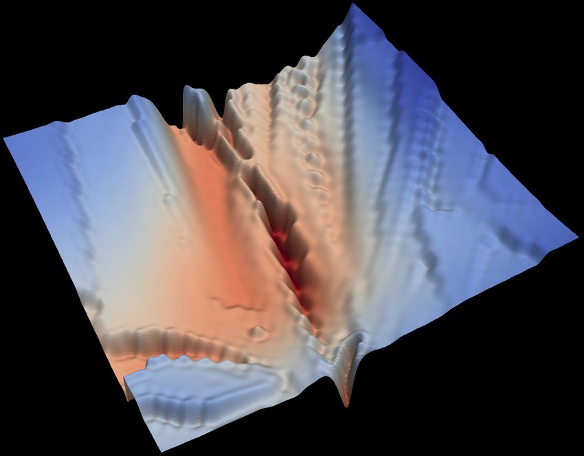
Under review as a conference paper at ICLR 2021
Figure 1: Left: 3D probability distribution tensor, only nonzero values are indicated with colored
cubes, all empty space is assumed to be filled with zero-valued cubes. Middle left: an example of
an additive transformation conditioned on x3 : y1 = x1 + bt1 (x3 )e, y2 = x2 + bt2 (x3 )e, y3 = x3 .
Middle right: an example of an additive transformation conditioned on x1 and x3 : y1 = x1 ,
y2 = x2 + bt2 (x1 , x3 )e, y3 = x3 . Right: a distribution tensor that a single additive transformation of
the form of (4) cannot generate from the cube on the left.
variable x = (x1 , x2 ), with x1 , x2 ∈ {0, 1}, and a data distribution given by
x1 \x2 0 1
0 0.1 0.3
px (x1 , x2 ) : . (5)
1 0.2 0.4
In order to map this probability distribution to an independent base distribution, the corresponding
probability matrix must be of rank one. In other words, given a sequence of functions f k : X 7→ X
with X = {0, 1}2 , the probability distribution of the random variable y = y K = f K ◦ f K−1 ◦ ... ◦
f 1 (x) should be represented by a matrix with linearly dependent columns or rows. This allows for a
factorization into an outer product of two vectors that represent the independent base distributions for
y1 and y2 . Since discrete flows can only permute probability mass tensors, the matrix corresponding
to py (y1 , y2 ) must be a permutation of the matrix in (5). However, there is no permutation of the
elements in (5) that results in a rank-one matrix. Therefore, Papamakarios et al. (2019) conclude that
discrete normalizing flows cannot map any distribution to a factorized base distribution.
However, one of the key assumptions made above is that the domain of f k is restricted to X = {0, 1}2 .
By extending X to a larger number of classes this example can in fact be factorized by a discrete
normalizing flow. More concretely, let us extend the domain to X = {0, 1, 2, 3}2 . The probability
distribution matrix of x is shown below, together with a permutation of rank 1.
0.1 0.3 0 0 0.1 0 0 0 0.1 1
0.2 0.4 0 0 0.2 0 0 0 0.2 0
px (x1 , x2 ) : → py (y1 , y2 ) : = ⊗ . (6)
0 0 0 0 0.3 0 0 0 0.3 0
0 0 0 0 0.4 0 0 0 0.4 0
This example illustrates that the number of classes that are considered valid for the discrete random
variables plays a crucial role in the flexibility of discrete flows. Here, we claim that this holds more
generally through the following two lemmas. First we show that by embedding the data into a space
with more possible values than present in the data itself, one can always construct an invertible
mapping to one-dimensional variable embedded in d dimensions, and that the resulting variable has a
distribution which is trivially factorized across all d dimensions.
Lemma 1. A d-dimensional discrete random variable x = (x1 , . . . , xd )T with d > 1 and xi ∈
{0, . . . , K (i) − 1}, distributed according to an arbitrary
Q distribution px (x), can be transformed
d (i)
to a one-dimensional random variable y ∈ {0, . . . , i=1 K − 1} with a number of classes
that scales exponentially with the dimension d through a bijective mapping f . Embedding y in d
dimensions through padding with d − 1 zeros, i.e. y = (y, 0, . . . , 0)T , the distribution over y is
Qd
trivially factorized across all dimensions: px (x) = py (f (x)) i=2 δyi ,0 with δi,j the Kronecker
delta distribution for all zero-padded dimensions.
Qd−1
The closed form of the mapping
Q is y= f (x) = x1 + K (1) x2 + K (1) K (2) x3 + · · · + i=1 K (i) xd ,
d (i)
such that y ∈ {0, . . . , i=1 K − 1}. See Appendix A for the full proof. Intuitively, given
enough classes, a factorized base distribution is obtained by “flattening” the hypercube that contains
4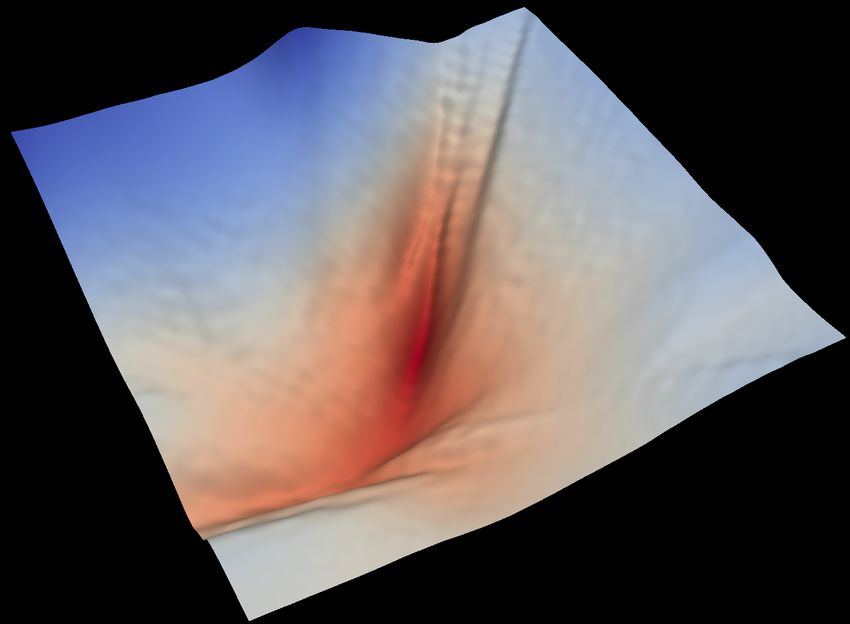
Under review as a conference paper at ICLR 2021

Figure 2: Visualization of an IDF that has learned to factorize the probability distribution of the toy
example in (5). Left: empirical densities of the data, the data transformed by one additive bijector,
and the data transformed by two additive bijectors. Right: similar to the left plot, but with data
sampled from the model.

all nonzero entries in the data distribution tensor (see left panel Figure 1) into one dimension. The
following lemma demonstrates that additive coupling layers as in (4) of integer discrete flows can
model such an invertible mapping.
Lemma 2. For a d-dimensional random variable x, translation operations of the form za = xa ,
zb = xb + bt(xa )e, with a and b denoting the indices of two splits of the variable x, are sufficient to
map x in an invertible manner to a random variable y = (y1 , 0, . . . , 0)T , which is a one-dimensional
variable embedded in d dimensions.

The formal proof is an induction on d and relies on 1) the fact that integer discrete flows embed the
discrete random variables into the integer lattice X = Zd , which always has a sufficient number
of classes (countably infinite), and 2) the observation that two translations are sufficient to map
two dimensions into a single dimension with more classes, see Appendix A. For a more intuitive
illustration, Figure 1 depicts the type of operations that a single additive bijector can and cannot
perform on a three-dimensional probability tensor. In Figure 2 we show that, although sensitive
to initialization, an IDF can be trained to factorize the toy example of (5). The first three panels
correspond to the data distribution and the intermediate and factorized final distributions produced by
the first and second coupling layer respectively. For architecture details see Appendix D.3.
As pointed out by Papamakarios et al. (2019), a discrete flow can only map a uniform base distribution
into a uniform data distribution due to its permutation property. Therefore, invertible discrete flows
require one-dimensional learnable distributions in order to be able to model all data distributions.
Note also that discrete flows as introduced by Tran et al. (2019) are designed for a finite number
of classes in X and therefore cannot factorize all distributions. Although not implemented in the
original work, this model class can in principle also be extended to embed the data into a space with a
larger finite number of possible values than present in the support of the data in order to help alleviate
this issue. Since IDFs treat the random variable as integers (with a countably infinite number of
classes) it does not have a limited factorization capacity. We therefore explore other directions for
potential improvements.

5    D OES GRADIENT BIAS HINDER OPTIMIZATION OF IDF S ?

In this section we investigate whether gradient bias is a problem when training IDF models. Hooge-
boom et al. (2019a) demonstrated that the performance of IDFs can deteriorate when the number
of coupling layers is too large, and that this does not occur in the continuous additive counterpart
without rounding operators or straight-through gradient estimators. The gradient bias induced by the
straight-through estimator was suggested to be the cause.
In our experiments we found that neither stochastic rounding nor replacing the identity function in the
straight-through estimator with a soft approximation of the rounding function improved the results.
To disentangle the effect of gradient bias of the straight-through estimator and the difficulty of discrete
optimization, we have trained IDFs and their continuous additive counterpart (without the rounding
operator and without a quantized base distribution) on CIFAR-10. We use different combinations of
translation activation functions and backward substitute functions in the straight-through estimator:
soft rounding, hard rounding and the identity function. The soft rounding function σT was modeled
with a superposition of scaled sigmoid functions and a temperature T that allows to interpolate
between the identity function (T = 1) and the rounding function T = 0, see Appendix C for more
details. The left plot in Figure 3 shows that the continuous model with an identity straight-through

                                                    5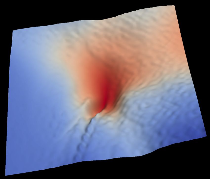
Under review as a conference paper at ICLR 2021

Figure 3: Left: Bits per dimension for models trained for 2000 epochs on CIFAR-10. Continuous
(cont) and discrete (disc) models are trained with different combinations of translations activation
functions (→) and backward (←) substitute functions for the straight-through estimators: a soft
rounding function (σT ), a hard rounding function (rnd) and the identity function (id). σT interpolates
between the identity function at T = 0 and the hard rounding function at T = 1. Right: Bits per
dimension of IDF models trained for 300K iterations (±960 epochs) with different architectures
for the translation networks in the coupling layers: convolutional neural networks, ResNets and
DenseNets. The models have 3 levels. The discrete ResNet model for 10 flows per level was unstable
so the result for this model is omitted. The models with the DenseNet architecture correspond to the
best models used by Hoogeboom et al. (2019a). The ConvNets and ResNets have approximately
equal number of parameters and depth as the DenseNets. Note that the ConvNets used to produce the
results in Fig. 5 of (Hoogeboom et al., 2019b) are much shallower. The DenseNet++ architectures
correspond to the proposed IDF++ model of Section 6.

gradient estimator consistently outperforms the continuous model without gradient bias. The discrete
model clearly also does not benefit from a soft-rounding operator in the straight-through estimator,
even though this estimator reduces the bias. Note that the continuous model trained with a hard
rounding function and identity straight-through estimator (→ rnd, ← id) performs worse than the
discrete model because the continuous model needs to maximize a lower bound to the likelihood.
We numerically study the significance of gradient bias in more detail on an extension of the two-
dimensional toy example of Section 4 to 8 bits with a model with two coupling layers. For details
on the 8-bit extension of the toy example see Appendix B and for architecture details see Appendix
D.3. We study the search directions using finite differences as an approximate gradient vector g fd
with elements g fd
                i = (L(θi + , θ /i ) − L(θi − , θ /i ))/2. Here L is the loss function averaged over
a single batch of data. For additive continuous flow models, g fd will approach the true loss gradient
∇θ L as  → 0. For discrete models, g fd can be thought of as a linear approximation of the loss
landscape in a trust-region of radius  around the current parameter vector θ.
We compare continuous flow models that are trained using the unbiased gradient ∇θ L with discrete
flow models that are trained using the straight-through gradient estimator g st . We estimate the
agreement between the (approximate) gradient and the finite difference approximation g fd for varying
trust-region size  at various stages of training and for varying bit-depth of the input data. We compute
the agreement of the (approximate) gradient directions with the cosine similarity g · g fd /||g||2 ||g fd ||2 ,
which can be interpreted as the uncentered correlation between the elements of g and g fd . As long
as the agreement is consistently positive, performing gradient descent with g is expected to reduce
the loss according to the trust-region approximation based on g fd . If the agreement is consistently
zero, or even negative, gradient descent with g is not expected to improve the training loss. The
agreements are estimated over multiple batches. As the base distribution parameters are not affected
by the gradient bias we only consider the gradients for the parameters of the bijectors.
Figure 4 shows the agreement between the finite-difference gradient and the straight-through gradient
of the discrete model and the agreement with the real gradient for the continuous model, at initial-
ization and after 3000 training iterations. The straight-through gradient estimator for 8-bit data is
always positively correlated with small but finite difference estimates, corroborating our results on
CIFAR-10 that the identity straight-through gradient estimator allows for good optimization. For
1-bit data the quality of the straight-through gradient estimator clearly deteriorates and the correlation
becomes zero or even negative. This is not surprising as the random variables and translations are in
practice modeled on the rescaled grid Z/2bits , leading to more coarse-grained rounding for lower bits.
As lossless compression mostly deals with source data in the higher bit ranges the poor performance

                                                      6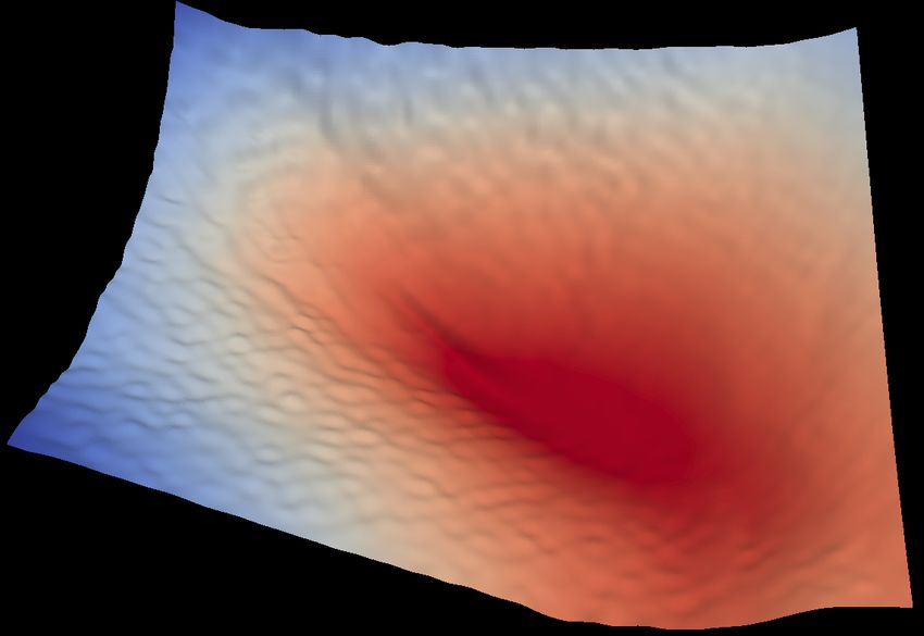
Under review as a conference paper at ICLR 2021

Figure 4: Top two panels: Agreement between the approximate (true) gradient and finite difference
gradient of the discrete (continuous) model at model initialization (left), and after 3000 training
iterations (right). The curves were obtained by averaging over 10 batches. The higher variance for
the 8-bit case is due to the larger number of different datapoints, leading to more variance in the data
batches. Bottom two panels: Visualization of the loss surface (left) and trajectory of the optimizer on
the loss surface (right) for the discrete model on the 1-bit toy example, following (Li et al., 2018).

for lower bit data is less relevant. The bottom two panels in Figure 4 show the loss surface and
optimization trajectory of a discrete model trained on the 1-bit data, suggesting that the optimization
landscape is hard to traverse for low bit-depths. See Appendix B for loss landscapes for 8-bit data
and for similar plots for the corresponding continuous models.
Finally, we observed that the performance degradation of IDF as a function of the number of coupling
layers is highly dependent on the architecture used for the translation networks in the coupling
layers. The right plot in Figure 3 shows the performance of continuous and discrete models with
identity straight-through estimators, under different coupling layer architectures: stacked convolutions,
ResNets (He et al., 2016) or DenseNets (Huang et al., 2017). All coupling layer architectures are
of approximately the same size and depth, and the DenseNet models have the same architecture as
the best model of (Hoogeboom et al., 2019b). The performance of the convolutional model clearly
deteriorates quicker than the ResNet and DenseNet models.
The results in this section show that gradient bias due to the straight-through estimator is less of a
problem than previously suggested. Alternative gradient estimators with less bias do not improve the
results, and our analysis on the toy examples shows that for data with large bit depths the straight-
through gradient estimates have positive correlation with finite difference estimates. We show that
the previously observed performance deterioration as a function of the number of coupling layers
is highly dependent on the architecture choice of the coupling layers. This motivates our search for
architectural changes that can help improve the performance of IDFs on lossless image compression.

6    I MPROVING I NTEGER D ISCRETE F LOWS FOR L OSSLESS C OMPRESSION
In this section we introduce changes to the architecture of IDF that improve its performance. We
briefly summarize the IDF architecture, for more detailed information see Appendix D. Similar to
other generative flow models, the architecture of IDF contains L levels. Each level l consists of a
space-to-depth transformation followed by a sequence of K alternating channel permutations and
additive coupling layers. For levels l = 1, ..., L − 1 the output random variable is split into two pieces,
with the second part serving as an input to the next level: [z (l) , y (l) ] = f (l,K) ◦ ... ◦ f (l,1) (y (l−1) ),
with y (0) = x. For the last level we simply have z (L) = f (L,K) ◦ ... ◦ f (L,1) (y (L−1) ). The combined

                                                        7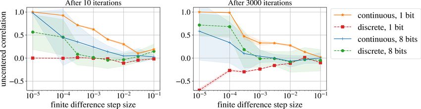
Under review as a conference paper at ICLR 2021

z = [z (1) , ..., z (L) ] denotes the latent representation of x. The distribution of z for 3 levels is
then factorized as p(z) = p(z (1) , z (2) , z (3) ) = p(z (3) )p(z (2) |y (2) )p(z (1) |y (1) ), which is equivalent
to p(z (3) )p(z (2) |z (3) )p(z (1) |z (2) , z (3) ). The conditional distributions are modeled as discretized
logistic distributions and the unconditional p(z (3) ) is modeled with a mixture of discretized logistics
with 5 components. Both the conditioning networks and the pre-quantized translations tθ in (4) are
modeled with DenseNets (Huang et al., 2017).
The first modification is to invert the channel permutations after every coupling layer. Although
inverting the permutation after each translation does not affect the coupling layers of the network, it
affects the way the data is split after each level and therefore influences the modeling of the conditional
distributions p(z (l) |y (l) ). By inverting the permutations one ensures that the split into y (l) and z (l)
happens along the channel direction of the space-to-depth transformed version of y (l−1) ; as such y (l)
and z (l) retain the spatial correlation structure of the original image presumably making it easier to
model the conditional distribution p(z (l) |y (l) ) (see visualization in Figure 10 of Appendix D).
The second change is an adaptation of the rezero trick by Bachlechner et al. (2020). The additive
bijectors of (4) are replaced by [y a , y b ] = [xa , xb + bαtθ (xa )e], where α is a learnable scalar
parameter initialized to zero, such that the bijectors are initialized to the identity function. The
mean and log-scale of the conditional discretized logistic distributions are parameterized as µ = γν,
log s = δ log σ with [ν, log σ] = DenseNetφ (y) and γ and δ learnable scalar parameters initialized
to zero.
The third modification consists of an alteration in the dense blocks that make up the translation and
logistic conditioning DenseNets by introducing group normalization layers (Wu & He, 2018) and
switching from ReLU activations (Nair & Hinton, 2010) to Swish activations (Ramachandran et al.,
2017):
       IDF: Conv1x1 → ReLU → Conv3x3 → ReLU
       IDF++: Conv1x1 → GroupNorm → Swish → Conv3x3 → GroupNorm → Swish
The trainability of deep neural networks such as flow models is strongly dependent on careful
initialization and normalization. Identity mapping initialization of flow models, which we achieve
by virtue of the rezero trick, is a known technique for improving training stability of these models
(Kingma & Dhariwal, 2018). The use of group normalization layers ensures that the dense blocks
within the coupling layers receive properly scaled and centered inputs. Combined with the Swish
activation function this allows DenseNet activations to remain non-zero and the coupling layers to
utilize their capacity more effectively. Empirically, these intuitions are supported by the fact that
collectively these modifications allow for the use of a higher base learning rate during training while
achieving better results. Finally, during training we also keep track of a slow exponential moving
average of the models weights, and use these average weights during evaluation.
Figure 3 shows the performance of models with the proposed modifications (DenseNet++) on the
validation set (consisting of 20% of the training set) on CIFAR-10 as a function of flows per level,
after 300K iterations. For this new architecture the performance of both the continuous and the
discrete version of the model deteriorates for 10 flows per level due to overfitting (see Fig. 11). These
results also show that the modifications allow for a more efficient use of the flow layers: for 300K
iterations the performance of the IDF++ model with a DenseNet++ architecture is on par with that of
the IDF model of Hoogeboom et al. (2019a) with DenseNet coupling layers.
To further corroborate this point, we have trained an IDF++ model with 4 and 8 flows per level until
convergence for CIFAR10, ImageNet-32 and ImageNet-64, and compared it with the baseline IDF
model with 8 flows per level and other related work in Table 1. To make a fair comparison against
other methods like local bits-back coding (LBB) by Ho et al. (2019b) we train our final models on
the entire training set without holding out part of the training set as a validation set. Although there
is no visible difference for the ImageNet-32 and ImageNet-64 datasets, more data does matter for
CIFAR-10: it reduces the model’s average negative log-likelihood in units of bits per dimension
(bpd) on the test set from 3.32 (as reported by Hoogeboom et al. (2019a)) to 3.30 for the baseline
IDF model. Table 1 displays the bpd resulting from compressing the latent representations z with
a range-based Asymmetric Numerical Systems (rANS) entropy coder (Duda, 2013). Results for
hand-designed codecs, models with bits-back coding and models without bits-back coding are shown
in separate groups. Where available, the bpd as predicted from the models negative log-likelihood is
indicated in brackets.

                                                         8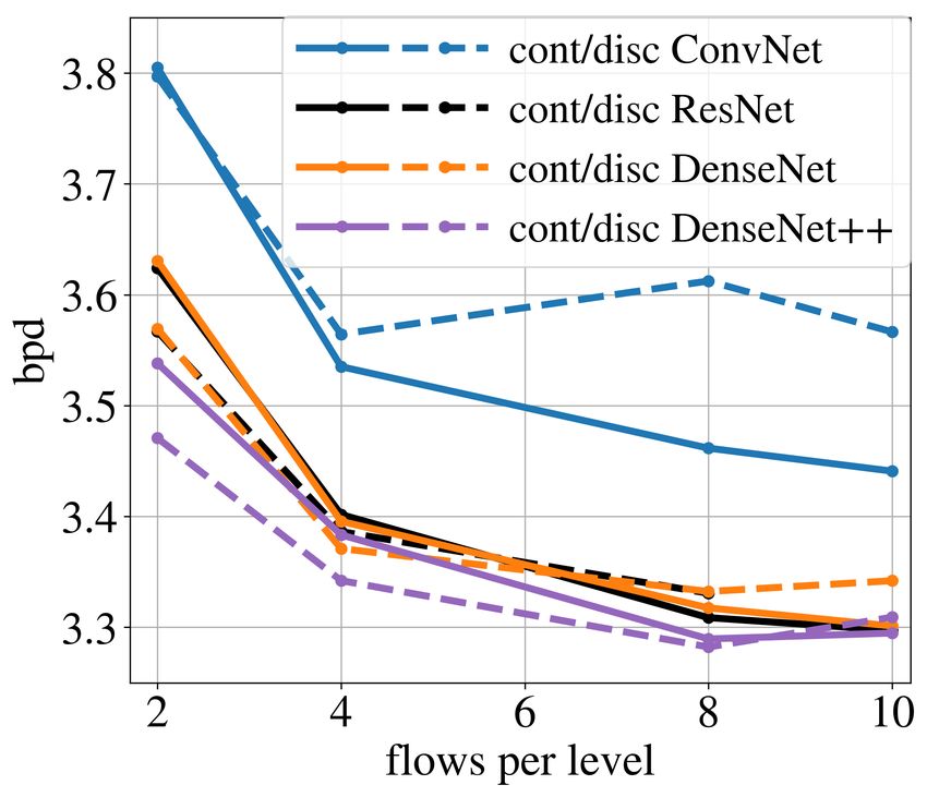
Under review as a conference paper at ICLR 2021

Table 1: Compression results in bits per dimension (bpd) for IDF++, hand-designed codecs and other
deep density estimators based on normalizing flows, super resolution and variational auto-encoders.
Where available, the bpd according to the model’s negative log-likelihood is indicated in parenthesis.
Results with a ∗ are taken from Townsend et al. (2019a), and those with † are taken from Hoogeboom
et al. (2019a). The IDF CIFAR-10 result indicated with ∗∗ is obtained by our implementation of IDF
with 100% of the training data used to train the model. In (Hoogeboom et al., 2019a) only 80% of
the training data was used to train the best CIFAR-10 model. All other results are from the original
papers.

    Compression models                        C IFAR -10        I MAGE N ET-32    I MAGE N ET-64
                                                   ∗                ∗
    PNG (Boutell & Lane (1997))               5.87             6.39               5.71∗
    JPEG-2000 (Rabbani (2002))                5.20†            6.48†              5.10†
    FLIF (Sneyers & Wuille (2016))            4.19∗            4.52∗              4.19∗
    B IT-S WAP (Kingma et al. (2019))         3.82 (3.78)      4.50 (4.48)          -
    H I LL O C (Townsend et al. (2019a))      3.56 (3.55)      4.20 (4.18)        3.90 (3.89)
    LBB (Ho et al. (2019b))                   3.12 (3.12)      3.88 (3.87)        3.70 (3.70)
    SR E C (Cao et al. (2020))                  -                -                4.29
    IDF (Hoogeboom et al. (2019a))            3.32 (3.30)∗∗    4.18 (4.15)        3.90 (3.90)
    IDF++, SMALL : 4 FLOWS PER LEVEL          3.32 (3.30)      4.18 (4.15)        3.85 (3.84)
    IDF++                                     3.26 (3.24)      4.12 (4.10)        3.81 (3.81)

The results show that, contrary to less-biased gradient estimators, the proposed architecture modifica-
tions in IDF++ improve the performance over IDF for 8 flows per level for all datasets. Furthermore,
the smaller IDF++ model with only 4 flows per level either performs on par or better than the
IDF baseline with 8 flows per level. This effectively reduces the number of parameters and time
required for a forward pass through the model by a factor of 2, and demonstrates that the proposed
modifications in IDF++ enable more efficient compression without sacrificing performance. For a
more detailed ablation on the contributions of the proposed modifications see Appendix E.

7    C ONCLUSION

In this paper we investigated several potential directions for improvement of integer discrete flows
for lossless compression. We analyzed the hypothesis and claims of recent works on the weaknesses
of this model class, and we showed that the claim by Papamakarios et al. (2019) that flows for
discrete random variables cannot factorize all distributions does not apply to integer discrete flows.
Furthermore, we demonstrated that the effect of gradient bias on optimization is less severe than
previously thought. Other gradient estimators with less bias do not improve optimization, and
a numerical analysis of the direction of the straight-through gradient estimates showed that they
correlate well with finite difference estimates for large-bit data. We also showed that the previously
observed performance deterioration with increasing depth of the flow model is highly dependent on
the architecture of the coupling layers. Motivated by this, we proposed several architecture changes
that improve the performance of IDFs on lossless image compression for an equal computational
budget. The proposed modifications lead to a more efficient flow-based compression model, as
evidenced by our results that show that an IDF++ model with half the number of flows compared to
the baseline IDF model performs on par or better.
Although we found that the simple straight-through gradient estimator outperformed all of the other
estimators that we considered, future work could consider other estimators inspired by universal
quantization and the statistics of quantization noise, similar to the work by Agustsson & Theis (2020).
Another important direction for future work is to further reduce the computational complexity of deep
density estimators. Although hand-designed codecs such as JPEG-2000 do not compress as well on
the datasets we consider, they (de)compress significantly faster and require significantly less memory
while not being tuned for each dataset. More work in directions like optimizing for (de)compression
speed (Cao et al., 2020) or generalizing learnable compressors to other datasets (Townsend et al.,
2019a) is needed to make deep density estimators more practical for source compression.

                                                  9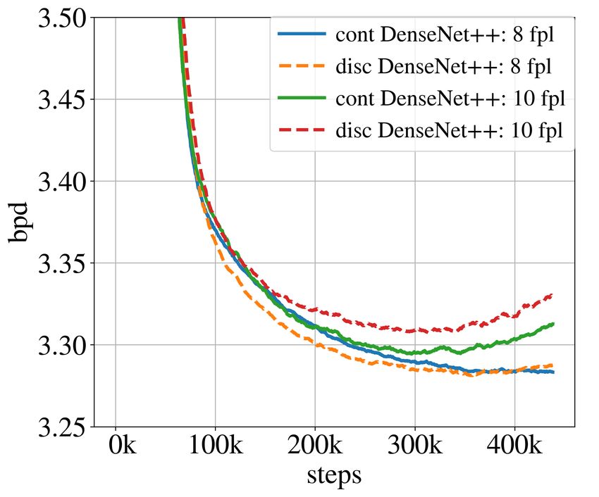
Under review as a conference paper at ICLR 2021

R EFERENCES
Martı́n Abadi, Ashish Agarwal, Paul Barham, Eugene Brevdo, Zhifeng Chen, Craig Citro, Greg S.
 Corrado, Andy Davis, Jeffrey Dean, Matthieu Devin, Sanjay Ghemawat, Ian Goodfellow, Andrew
 Harp, Geoffrey Irving, Michael Isard, Yangqing Jia, Rafal Jozefowicz, Lukasz Kaiser, Manjunath
 Kudlur, Josh Levenberg, Dandelion Mané, Rajat Monga, Sherry Moore, Derek Murray, Chris Olah,
 Mike Schuster, Jonathon Shlens, Benoit Steiner, Ilya Sutskever, Kunal Talwar, Paul Tucker, Vincent
 Vanhoucke, Vijay Vasudevan, Fernanda Viégas, Oriol Vinyals, Pete Warden, Martin Wattenberg,
 Martin Wicke, Yuan Yu, and Xiaoqiang Zheng. TensorFlow: Large-scale machine learning on
 heterogeneous systems, 2015. URL https://www.tensorflow.org/. Software available
 from tensorflow.org.
Eirikur Agustsson and Lucas Theis. Universally quantized neural compression. arXiv:2006.09952,
  2020.
Jimmy Lei Ba, Jamie Ryan Kiros, and Geoffrey E Hinton. Layer normalization. arXiv:1607.06450,
  2016.
Thomas Bachlechner, Bodhisattwa Prasad Majumder, Huanru Henry Mao, Garrison W. Cottrell, and
  Julian McAuley. ReZero is All You Need: Fast Convergence at Large Depth. arXiv:2003.04887,
  2020.
Thomas Boutell and T Lane. PNG (portable network graphics) specification version 1.0. Network
  Working Group, 1997.
Sheng Cao, Chao-Yuan Wu, and Philipp Krähenbühl. Lossless Image Compression through Super-
  Resolution. arXiv:2004.02872, 2020.
Scott Saobing Chen and Ramesh A. Gopinath. Gaussianization. In Advances in Neural Information
  Processing Systems 13. 2001.
Peter Deutsch. DEFLATE compressed data format specification version 1.3, 1996.
Laurent Dinh, David Krueger, and Yoshua Bengio. NICE: Non-linear independent components
  estimation. arXiv:1410.8516, 2014.
Laurent Dinh, Jascha Sohl-Dickstein, and Samy Bengio. Density estimation using real NVP.
  arXiv:1605.08803, 2016.
Jarek Duda. Asymmetric numeral systems. arXiv:0902.0271, 2009.
Jarek Duda. Asymmetric numeral systems: entropy coding combining speed of huffman coding with
   compression rate of arithmetic coding. arXiv:1311.2540, 2013.
Kaiming He, Xiangyu Zhang, Shaoqing Ren, and Jian Sun. Deep residual learning for image
  recognition. In Proceedings of the IEEE conference on computer vision and pattern recognition,
  2016.
Geoffrey E Hinton and Drew Van Camp. Keeping the neural networks simple by minimizing the
  description length of the weights. In Proceedings of the sixth annual conference on Computational
  learning theory, 1993.
Jonathan Ho, Xi Chen, Aravind Srinivas, Yan Duan, and Pieter Abbeel. Flow++: Improving flow-
  based generative models with variational dequantization and architecture design. arXiv:1902.00275,
  2019a.
Jonathan Ho, Evan Lohn, and Pieter Abbeel. Compression with Flows via Local Bits-Back Coding.
  In Advances in Neural Information Processing Systems 32, 2019b.
Emiel Hoogeboom, Jorn Peters, Rianne van den Berg, and Max Welling. Integer Discrete Flows and
  Lossless Compression. In Advances in Neural Information Processing Systems 32, 2019a.
Emiel Hoogeboom, Rianne Van Den Berg, and Max Welling. Emerging Convolutions for Generative
  Normalizing Flows. In Proceedings of the 36th International Conference on Machine Learning,
  2019b.

                                                10
Under review as a conference paper at ICLR 2021
G. Huang, Z. Liu, L. Van Der Maaten, and K. Q. Weinberger. Densely Connected Convolutional
Networks. In 2017 IEEE Conference on Computer Vision and Pattern Recognition (CVPR), 2017.
Sungwon Kim, Sang-gil Lee, Jongyoon Song, Jaehyeon Kim, and Sungroh Yoon. FloWaveNet: A
generative flow for raw audio. arXiv:1811.02155, 2018.
Diederik P. Kingma and Jimmy Ba. Adam: A method for stochastic optimization. arXiv:1412.6980,
2014.
Diederik P Kingma and Max Welling. Auto-encoding variational bayes. arXiv:1312.6114, 2013.
Durk P Kingma and Prafulla Dhariwal. Glow: Generative flow with invertible 1x1 convolutions. In
Advances in Neural Information Processing Systems, 2018.
Friso H Kingma, Pieter Abbeel, and Jonathan Ho. Bit-swap: Recursive bits-back coding for lossless
compression with hierarchical latent variables. arXiv:1905.06845, 2019.
Manoj Kumar, Mohammad Babaeizadeh, Dumitru Erhan, Chelsea Finn, Sergey Levine, Laurent
Dinh, and Durk Kingma. Videoflow: A flow-based generative model for video. arXiv:1903.01434,
2019.
Hao Li, Zheng Xu, Gavin Taylor, Christoph Studer, and Tom Goldstein. Visualizing the loss landscape
of neural nets. In Advances in Neural Information Processing Systems, 2018.
Fabian Mentzer, Eirikur Agustsson, Michael Tschannen, Radu Timofte, and Luc Van Gool. Practical
full resolution learned lossless image compression. In Proceedings of the IEEE Conference on
Computer Vision and Pattern Recognition, 2019.
Fabian Mentzer, Luc Van Gool, and Michael Tschannen. Learning Better Lossless Compression
Using Lossy Compression. arXiv:2003.10184, 2020.
Vinod Nair and Geoffrey E. Hinton. Rectified Linear Units Improve Restricted Boltzmann Machines.
In Proceedings of the 27th International Conference on International Conference on Machine
Learning, 2010.
Aaron van den Oord, Nal Kalchbrenner, and Koray Kavukcuoglu. Pixel recurrent neural networks.
arXiv:1601.06759, 2016.
George Papamakarios, Eric Nalisnick, Danilo Jimenez Rezende, Shakir Mohamed, and Balaji Laksh-
minarayanan. Normalizing Flows for Probabilistic Modeling and Inference. arXiv:1912.02762,
2019.
Majid Rabbani. JPEG2000: Image compression fundamentals, standards and practice. Journal of
Electronic Imaging, 2002.
Richard Rabbat. WebP, a new image format for the Web, 2010. URL https://blog.chromium.
org/2010/09/webp-new-image-format-for-web.html.
Prajit Ramachandran, Barret Zoph, and Quoc V. Le. Searching for Activation Functions.
arXiv:1710.05941, 2017.
Danilo Rezende and Shakir Mohamed. Variational Inference with Normalizing Flows. In Proceedings
of the 32nd International Conference on Machine Learning, 2015.
Tim Salimans, Andrej Karpathy, Xi Chen, and Diederik P Kingma. PixelCNN++: Improving the
PixelCNN with discretized logistic mixture likelihood and other modifications. arXiv:1701.05517,
2017.
Jon Sneyers and Pieter Wuille. FLIF: Free lossless image format based on MANIAC compression.
In 2016 IEEE International Conference on Image Processing (ICIP). IEEE, 2016.
Lucas Theis and Matthias Bethge. Generative image modeling using spatial lstms. In Advances in
Neural Information Processing Systems, 2015.
11Under review as a conference paper at ICLR 2021
Lucas Theis, Aron van den Oord, and Matthias Bethge. A note on the evaluation of generative models.
arXiv:1511.01844, 2015.
James Townsend. A tutorial on the range variant of asymmetric numeral systems. arXiv:2001.09186,
2020.
James Townsend, Thomas Bird, Julius Kunze, and David Barber. HiLLoC: Lossless Image Compres-
sion with Hierarchical Latent Variable Models. arXiv:1912.09953, 2019a.
James Townsend, Tom Bird, and David Barber. Practical lossless compression with latent variables
using bits back coding. arXiv:1901.04866, 2019b.
Dustin Tran, Keyon Vafa, Kumar Agrawal, Laurent Dinh, and Ben Poole. Discrete Flows: Invertible
Generative Models of Discrete Data. In Advances in Neural Information Processing Systems 32,
2019.
Benigno Uria, Iain Murray, and Hugo Larochelle. RNADE: The real-valued neural autoregressive
density-estimator. In Advances in Neural Information Processing Systems 26. 2013.
Benigno Uria, Iain Murray, and Hugo Larochelle. A deep and tractable density estimator. In
International Conference on Machine Learning, 2014.
Yuxin Wu and Kaiming He. Group Normalization. Lecture Notes in Computer Science, 2018.
12Under review as a conference paper at ICLR 2021
Supplementary Material of “IDF++: Analyzing and Improving
Integer Discrete Flows for Lossless Compression”
A PPENDIX A F LEXIBILITY OF INTEGER DISCRETE FLOWS
The proof of Lemma 1 can be done in two ways, one is by giving the exact mapping, and the second
way is through induction. We include both below as well as the proof for Lemma 2.
(1) (1) (2)
Q by y =f (x) = x1 + K x2 + K K x3 +
Proof of Lemma 1. The invertible mapping is given
Qd−1 (i) d (i)
· · · + i=1 K xd , with a maximum value of i=1 K − 1 and minimum value of zero. Given
P
d j−1
y, each element xi can be obtained recursively: xi = y − j=i+1 K x j //K i−1 . Through
the change of variables formula we know that py (y) = px (f −1 (y)), which combined with zero
padding to embed in d dimensions leads to the desired factorized distribution in d dimensions.
Alternative proof of Lemma 1. An alternative proof is via induction on d.
Base case: Let us start with d = 2, we have the random variable x = (x1 , x2 )T with x1 ∈
{0, ..., K (1) − 1} and x2 ∈ {0, ..., K (2) − 1}. x is distributed according to px (x1 , x2 ). The
following function can map this random variable to a one-dimensional random variable y with
y ∈ {0, . . . , K (1) K (2) − 1}: y = x1 + K (1) x2 . Given y, x1 and x2 can be recovered through
x2 = y//K (1) and x1 = y − K (1) x2 , where // refers to integer division.
General case: Now let us assume that the lemma holds for d = n, and examine the case of
d = n + 1: x = (x1 , ..., xn , xn+1 )T with xi ∈ {0, ..., K (i) }. Then the following transformation
maps to an n-dimensional random variable y = (y1 , . . . yn )T : yi = xi for i = {1, . . . , n − 1}
and yn = xn + K (n) xn+1 . x can be recovered from y through xi = yi for i = {1, . . . , n − 1}
and xn+1 = yn //K, xn = yn − Kxn+1 . We have y1 , ..., yn−1 ∈ {0, ..., K (i) − 1} and yn ∈
{0, ..., K (n) K (n−1) − 1}. As we assumed that we can transform an n-dimensional random variable
to a one-dimensional random variable in an invertible manner, this concludes that we can also do so
for the d = n + 1 case.
Proof of Lemma 2. We will prove this via induction on d.
Base case: Let us start again with d = 2. x = (x1 , x2 )T with xi ∈ {0, . . . , K (i) } can be transformed
into a random variable y = (y1 , 0)T in an invertible manner with two translation operations of
the form za = xa , zb = xb + bt(xa )e, where either (a, b) = (1, 2) or (a, b) = (2, 1). The
first translation is given by z1 = x1 + K (1) x2 , z2 = x2 , followed by y1 = z1 = x1 + K (1) x2 ,
y2 = x2 − (x1 + K (1) x2 )//K (1) = x2 − x2 = 0.
General case: Let us assume translations are sufficient for d = n. We can then transform a d = n + 1
dimensional variable x = (x1 , . . . , xn , xn+1 )T in an invertible manner to a random variable that is
effectively n-dimensional: y = (y1 , . . . , yn , 0) with two translations operations: The first translation
is:
zi = xi for i ∈ {1, . . . , n − 1, n + 1}
zn = xn + K (n) xn+1 , (7)
followed by the second translation:
yi = zi for i ∈ {1, . . . , n}
yn+1 = zn+1 − zn //K (n) = xn+1 − (xn + K (n) xn+1 )//K (n) = xn+1 − xn+1 = 0. (8)
Which results in yi = xi for i ∈ {1, ..., n − 1} and yn = xn + K (n) xn+1 . As we assumed integer
translations were sufficient to map an n-dimensional variable like (y1 , . . . , yn )T to a one-dimensional
random variable embedded in n dimensions in an invertible manner, we have now proven that this
also holds for d = n + 1.
13Under review as a conference paper at ICLR 2021
A PPENDIX B L EARNING TOY EXAMPLES
B.1 G RADIENT BIAS ON THE TOY EXAMPLE
The toy example that is discussed in Section 4 has a probability distribution with nonzero probabilities
for xi ∈ {0, 1}. With only two values per dimension with nonzero probability the data is effectively
1-bit quantized. Here we use an extension of this toy example for input data that is quantized to a
higher bit-depth. This can be done by modeling the probability masses with log-linearly spaced logits
in the interval (0, 1). The resulting distributions for several bit-depths are shown in Fig. 5.
1 bit 2 bits 4 bits 0
8 bits
2 2
0 32
1
1 64
0 4
0 96
1
8 128
x1
1 2
160
3 12
2 192
4
3 224
5 16
256
2 1 0 1 2 3 2 1 0 1 2 3 4 5 0 4 8 12 16 0 32 64 96 128 160 192 224 256
x2 x2 x2 x2
Figure 5: probability distribution of the extension of the toy example of Eq. (5) to more bits.
B.2 L OSS LANDSCAPE AND OPTIMIZER TRAJECTORY
In Section 5, we presented the visualization of the loss landscape and the optimization trajectory of
the discrete model on a toy example with 1-bit data. The details on how these plots were obtained
will be explained in this section. Navigating through a loss landscape that is affected by quantization
operators can be challenging due to discontinuities. To illustrate this effect, we visualize the loss
landscape and the optimization path for the discrete and continuous models trained on the 1-bit and
8-bit toy examples. We use the method proposed by Li et al. (2018), where for given model parameters
θ ∗ , we choose two direction vectors θ 1 and θ 2 and plot the value of f (α, β) = L(θ ∗ + αθ 1 + βθ 2 ).
To choose the direction vectors, we use model parameters at different stages of training. Let θ ∗i be
model parameters after iteration i. Given the set of parameters for n iterations, we apply PCA to the
matrix M = [θ ∗0 − θ ∗n , . . . , θ ∗n−1 − θ ∗n ] and select the two most explanatory directions as θ 1 and θ 2 .
The results for the 1-bit toy example are shown in the left two panels of Figure 4 for the discrete flow
model. Figure 6 shows similar plots for the continuous case, demonstrating a much smoother loss
landscape. Figure 4 suggests that discrete models with unlucky initializations can easily end up in a
local minimum from which it is hard to escape due to sharp cliffs in the loss landscape. Figures 7 and
8 show a significantly less pronounced difference between the loss landscape of the continuous and
discrete model for the 8-bit toy example. This supports our observation in Section 5 that the gradient
bias is less of an issue at higher bit-depths.
Figure 6: Visualization of the trajectory of the optimization on the loss surface (Li et al., 2018) for
the continuous model for the toy example with 1-bit data.
14Under review as a conference paper at ICLR 2021
Figure 7: Visualization of the trajectory of the optimization on the loss surface (Li et al., 2018) for
the discrete model for the toy example with 8-bit data.
Figure 8: Visualization of the trajectory of the optimization on the loss surface (Li et al., 2018) for
the continuous model for the toy example with 8-bit data.
A PPENDIX C S OFT ROUNDING FUNCTION
The soft rounding function σT that is used in Section 5 is given by
2
(x − bxc) − T1
σ T
σT (x) = bxc + . (9)
σ T1 − σ − T1
The soft rounding function is depicted in Figure 9 for different temperatures.
Figure 9: Soft rounding function σT for different temperatures T . In the limit T = 0 the soft
rounding function reduces to the hard rounding function b·e. At T = 1 the soft rounding function is
indistinguishable from the identity function.
15Under review as a conference paper at ICLR 2021
A PPENDIX D A RCHITECTURES
D.1 A RCHITECTURE AND TRAINING DETAILS OF IDF
The architecture of IDF consists of L levels, each consisting of an alternating sequence of channel
permutations and additive bijectors. More specifically, the architecture of level l of IDF is built up as
follows:
×K
z }| {
(l−1)
y → space-to-depth → {Permute → Additive transform} → [z (l) , y (l) ].
Except for the last level, the output random variable is split into two equal halves [z (l) , y (l) ], where
only y (l) is transformed by the next level. Furthermore, y (0) = x and z = [z (1) , . . . , z (L) ] denotes
the latent representation of x. Inside the additive transformations of (4) the prequantized translations
are modeled using DenseNets (Huang et al., 2017) with dense blocks of the following structure:
Dense block: Conv1x1 → ReLU → Conv3x3 → ReLU.
All DenseNets have a depth of 12 blocks and 512 channels. The additive bijector splits the random
variable into two parts along the channel dimension with splitting fractions 3/4 and 1/4 for the
untransformed and transformed parts of the random variable. After translating, the resulting variables
are concatenated again along the channel axis.
The distribution of z for L levels is factorized as p(z) = p(z (L) )p(z (L−1) |y (L−1) ) . . . p(z (1) |y (1) ),
which is equivalent to p(z (L) )p(z (L−1) |z (L) ) . . . p(z (1) |z (2) , . . . z (L) ). All conditional distributions
are modeled with discretized logistic distributions. The unconditional distribution p(z (L) ) is mod-
eled with a mixture of discretized logistics with five components. The log-scale and mean of the
conditional logistic distributions are modeled as the outputs of DenseNets with the same structure as
the DenseNets of the prequantized translations: [ν, log σ] = DenseNetφ (y). Note that instead of
modeling the random variables as integers (x ∈ Zd ), they are modeled as discrete random variables
on a grid with bin-width 1/256 (x ∈ Zd /256).
The model is trained with the Adamax optimizer (Kingma & Ba, 2014) with an exponential learning
rate schedule with base learning rate equal to 1 × 10⁻³ and a linear warmup phase of 10 epochs.
See Table 2 for more details on the learning rate decay, the number of levels, the batch size and the
number of epochs used for training.
Table 2: Architecture and training settings for IDF. Table adapted from Hoogeboom et al. (2019a).
Note that we used a batch size of 128 for Cifar-10 instead of 256 as used in the original work, while
still reproducing the same number as reported by Hoogeboom et al. (2019a). For ImageNet-32 and
ImageNet-64 the batch sizes are the same as in the original work (Hoogeboom et al., 2019a).
Dataset Levels L Batch size lr decay Epochs
CIFAR-10 3 128 0.999 2000
ImageNet-32 3 256 0.99 100
ImageNet-64 4 64 0.99 10
Range-based Asymmetric Numerical Systems (rANS) (Duda, 2009; 2013; Townsend, 2020) is
used for lossless compression of the latent variables z = [z (1) , . . . , z (L) ] by using the probability
distribution p(z) = p(z (L) )p(z (L−1) |y (L−1) ) . . . p(z (1) |y (1) ) corresponding to the model’s multi-
level structure.
D.2 A RCHITECTURE AND TRAINING DETAILS OF IDF++
In IDF++, each of the K blocks containing a permutation and additive bijector has an additional
inverse channel permutation to ensure that the output random variable has the same spatial and
channel ordering as the input random variable:
×K
z }| {
(l−1)
y → space-to-depth → {Permute → Additive transform → Inverse permute} → [z (l) , y (l) ].
16Under review as a conference paper at ICLR 2021
The inversion of each permutation inside a level ensures that the splitting at the end of each level
is done along the channel dimension of a space-to-depth transformed image, enabling the condi-
tional distributions to be able to use the spatial correlation between pixels. See Figure 10 for a
visualization. The dense blocks of the DenseNets for the prequantized translations and the condi-
tional discretized logistics have additional group normalization layers (Wu & He, 2018) and Swish
activations (Ramachandran et al., 2017) instead of ReLU activations (Nair & Hinton, 2010):
Dense block: Conv1x1 → GroupNorm → Swish → Conv3x3 → GroupNorm → Swish.
The number of groups for each group normalization layer are determined as follows: if the number of
channels of the group normalization layer is divisible by 3 then 3 groups are used, else if it is divisible
by 2 then 2 groups are used, and finally if it is neither divisible by 3 or 2 then a single group is used.
The additive bijectors in (4) are adjusted to include a learnable scalar parameter that ensures initial-
ization to the identity operator, similar to the rezero trick by Bachlechner et al. (2020):
ya xa
= . (10)
yb xb + btθ (αxa )e
Here α is a learnable scalar parameter initialized to zero. The mean and log-scale of the conditional
discretized logistic distributions are parameterized as µ = γν, log s = δ log σ with [ν, log σ] =
DenseNetφ (y). γ and δ are learnable scalar parameters initialized to zero, such that the scale is
initialized to one and the mean is initialized to zero.
The combination of the rezero trick and the group normalization layers allows us to use a larger base
learning rate of 2 × 10⁻³ in the exponential decayed learning rate schedule. For Cifar-10, the IDF++
(a)
1 2 3 4
5 6 7 8
9 10 11 12
13 14 15 16
(b)
1 3
2 4
9 11 5 7
6 8
10 12
chan 13 15
n 14 16
el dim
ensio
n
(c)
5
6
7
8
13 14
chann 15
el dim 16
ension
Figure 10: Schematic visualization of the effect of inverse permutations on the IDF++ architecture.
In a multi-level IDF++ model the original image (a) undergoes a space-to-depth transformation (b),
after which at the end of the first level half of the dimensions (blue tones) are factored out and their
conditional distribution based on the remaining dimension (green tones) is learned. This procedure
is repeated for the remaining dimensions (c) in the next level where again half the dimensions
(light green) are factored out and their conditional distribution is modelled based on the remaining
dimensions (dark green). By inverting permutations introduced in the coupling layers of each level
we guarantee that the spatial structure of the original image is preserved at all levels. Specifically,
with this structure, the factored out and remaining dimensions correspond to nearby rows of the
original image. We expect that the spatial correlation present in nearby rows is effectively leveraged
by the conditional distributions parameterized with convolutions, leading to better results.
17You can also read