Context-Aware Symptom Checking for Disease Diagnosis Using Hierarchical Reinforcement Learning - Stanford InfoLab
←
→
Page content transcription
If your browser does not render page correctly, please read the page content below
Context-Aware Symptom Checking for Disease Diagnosis
                         Using Hierarchical Reinforcement Learning

            Hao-Cheng Kao∗                                 Kai-Fu Tang∗                       Edward Y. Chang
        HTC Research & Healthcare                    HTC Research & Healthcare            HTC Research & Healthcare
        haocheng kao@htc.com                          kevin tang@htc.com                  edward chang@htc.com

                           Abstract                                    The primary goal of a symptom checker is to achieve
                                                                    high disease-prediction accuracy. Attaining the best possi-
  Online symptom checkers have been deployed by sites such
  as WebMD and Mayo Clinic to identify possible causes and          ble accuracy requires full information about a patient, in-
  treatments for diseases based on a patient’s symptoms. Symp-      cluding not only his/her symptoms, but also his/her medical
  tom checking first assesses a patient by asking a series of       record, family medical history, and lab tests. However, an
  questions about their symptoms, then attempts to predict po-      online symptom checker may only be able to obtain a list of
  tential diseases. The two design goals of a symptom checker       symptoms, and therefore must rely on partial information.
  are to achieve a high accuracy and intuitive interactions. In     This lack of information often means the online symptom
  this paper we present our context-aware hierarchical rein-        checker cannot attain extremely high accuracy. At the same
  forcement learning scheme, which significantly improves ac-       time, even obtaining a list of symptoms in a user friendly
  curacy of symptom checking over traditional systems while         manner is a challenge, since there are over one hundred dif-
  also making a limited number of inquiries.
                                                                    ferent medical symptoms, and few patients may be willing
                                                                    to fill out such a long symptom questionnaire. Consequently,
                       Introduction                                 this problem leads to the second requirement for an effective
With the quantity of information available online, self-            symptom checker, good user experience. The primary con-
diagnosis of health related ailments has become increas-            sideration in achieving good user experience is for a symp-
ingly prevalent. According to a survey in 2012 (Semigran            tom checker to make only a limited number of inquiries.
et al. 2015), 35% of U.S. adults in the U.S. have attempted         The design goal is then to maximize information gain when
to self-diagnose their ailments through online services This        only a limited number of symptom inquiries can be made to
process often starts by searching a particular symptom on a         achieve high diagnosis accuracy.
search engine. While online searches have fast accessibility           In previous works (Kononenko 2001; Kohavi 1996;
and require no cost, search quality can potentially be dis-         Kononenko 1993), Bayesian inference and decision trees as
satisfactory since search results could be irrelevant, impre-       well as entropy or impurity functions were proposed to se-
cise or even incorrect.                                             lect disease symptoms and to perform diagnoses. However,
   As stated in (Ledley and Lusted 1959), there are three           these works generally considered only local optimums by
components in a disease diagnosis process: (i) medical              some means of greedy or approximation schemes. These ap-
knowledge, (ii) signs and symptoms presented by the pa-             proaches often result in compromised accuracy. Expert sys-
tient, and (iii) the final diagnosis itself. We refer to such       tems are also used in medical diagnosis systems (Hayashi
processes as symptom checking, and refer to an agent ca-            1991). In this regime, rule-based representations are ex-
pable of performing such diagnoses as a symptom checker.            tracted from human knowledge or medical data. The final
In a symptom checker, a medical knowledge base serves as            inference quality depends on the quality of the extracted
the source of medical knowledge, which depicts the proba-           rules. For example, in (Hayashi 1991), if-else rules are ex-
bilistic relationship between symptoms and diseases. An in-         tracted from fuzzy neural networks learned from medical
ference engine is responsible for formulating symptom in-           data. Their rule-based representation focuses on knowledge
quiries, collecting patient information, and then performing        acquisition and does not pursue a shorter section of interac-
diagnosis by utilizing both the individual’s information and        tions with users. Our prior work (Tang et al. 2016) proposes
the medical knowledge base. If the prediction confidence is         neural symptom checking, adopting reinforcement learning
not high, the inference engine may suggest conducting rel-          to simultaneously conduct symptom inquiries and diagnose.
evant lab tests to facilitate diagnosis. Finally, the diagnosis     The optimization objective captures a combination of in-
process outputs a list of potential diseases that the patient       quiry length and diagnosis accuracy. Though our top-1 accu-
may have.                                                           racy reaches 48% (for 73 diseases), which is higher than the
   ∗
     The first two authors contributed equally to this paper.       34% average accuracy achieved by online services surveyed
Copyright c 2018, Association for the Advancement of Artificial     by a Harvard report (Semigran et al. 2015), substantial room
Intelligence (www.aaai.org). All rights reserved.                   exists for further improvement. (Table 1 presents details.)
Online Services #Diseases Accuracy Reinforcement Learning Formulation
Esagil 100 20% We regard a symptom checker as an agent solving a sequen-
MEDoctor 830 5% tial decision problem. This agent interacts with a patient
Mayo Clinic N/A 36% as follows: Initially, the agent is provided with a symptom
WebMD N/A 17% that the patient may have from the set of all symptoms I.
This provided symptom is regarded as the initial symptom.
Harvard Report (Avg.) N/A 34% In each time step, the agent chooses a symptom i ∈ I to
inquire the patient about. The patient then responds to the
Table 1: The current status of online diagnosis services eval- agent with a true/false answer indicating whether he/she is
uated by the Harvard report (Semigran et al. 2015). The top- suffering from that particular symptom. At the end of the
1 accuracies of representative sites are shown in percentages. diagnosis process, the agent predicts a disease d that the pa-
Note that Esagil and MEDoctor are the only services that ex- tient may have from the set of all diseases D.
plicitly disclose the number of their supported diseases. The The goal of the agent is to use as few steps as possi-
four listed services require a full list of the patients symp- ble while achieving high prediction accuracy. To this end,
toms. our prior work in (Tang et al. 2016) employs reinforcement
learning (Sutton and Barto 1998) and formulates this prob-
lem as a Markov decision process (MDP).
In this work, we introduce two novel enhancements to im- Formally, in time step t, the agent receives a state st and
prove diagnosis accuracy. First, we introduce a latent layer then selects an action at from a discrete action set A accord-
using anatomical parts. We employ hierarchical reinforce- ing to a policy π. In our formulation, A = I ∪ D. In each
ment learning to use a committee of anatomical parts to time step t, the agent receives a scalar reward rt . If at ∈ I,
make a joint diagnostic decision. While each anatomical part the agent performs an inquiry. If the inquiry is repeated, i.e.,
model is capable of selecting symptoms to inquire and diag- if at = at0 for some t0 < t, rt = −1 and the interaction
nose within the expertise of its anatomical part, each can is terminated; otherwise rt = 0 and the state is updated ac-
also inquire about different symptoms in a given state. Our cording to the response from the patient. If at ∈ D, the agent
proposed model utilizes a master model to select the specific performs a disease prediction and the interaction is termi-
anatomical part on which to perform inquiries at each inter- nated. In this case, rt = 1 if the predicted disease is correct;
action step. Our second enhancement is to introduce con- otherwise rt = 0.
text into the model and make our symptom checker context The goal is to find an optimal policy such that the agent
aware. The contextual information includes, but is not lim- maximizes the expected discounted total reward, i.e., the ex-
ited to, three aspects about a patient: who, when, and where. P∞ t0 −t
pected return Rt = t0 =t γ rt0 , where γ ∈ [0, 1] is a
The who aspect includes a person’s demographic informa- discount factor. The state-action Q-value function
tion (e.g., age and gender), heredity (characterized by ge-
netic data), and medical history. The when aspect can be Qπ (s, a) = E[Rt | st = s, at = a, π]
characterized by a distribution of diseases in the time of
is the expected return of performing an action a in a state s
year. The where aspect can be characterized by a distribution
following a policy π. Given that the Q-value is the sum of
of diseases from coarse to fine location granularities (e.g.,
an immediate reward and a discounted next-step Q-value, it
by country, city, and/or neighborhood). Any joint distribu-
can be rewritten as a recursive equation:
tions of any combinations of the who, when and where as-
pects can be formulated and quantified into a context-aware Qπ (s, a) = Es0 [r + γEa0 ∼π(s0 ) [Qπ (s0 , a0 )] | s, a, π]
model. Empirical studies on a simulated dataset show that
our proposed model drastically improves disease prediction where s0 and a0 are the state and action in the next time step,
accuracy by a significant margin (for top-1 prediction, the respectively.
improvement margin is 10% for 50 common diseases1 and The optimal Q-value is the maximum Q-value among all
5% when expanding to 100 diseases). possible policies: Q∗ (s, a) = maxπ Qπ (s, a). Also, it can
The rest of this paper is organized into five sections. be shown that the optimal Q-value obeys the Bellman equa-
We first briefly review formulating symptom checking in tion:
a reinforcement learning problem. We then introduce our Q∗ (s, a) = Es0 [r + γ max Q∗ (s0 , a0 ) | s, a].
0
proposed hierarchical ensemble model of anatomical parts. a
Next, we present the context-aware model. The experiment A policy π is optimal if and only if for every state and action,
section presents our results. An earlier version of our symp- Qπ (s, a) = Q∗ (s, a). In finite MDPs, such optimal policy
tom checker is employed in our DeepQ Tricorder (Chang always exists. Moreover, an optimal policy can be deduced
et al. 2017), which was awarded second prize in the Qual- deterministically by
comm Tricorder XPrize Competition (Qualcomm 2017). Fi-
nally, we offer our concluding remarks. π ∗ (s) = arg max Q∗ (s, a).
a∈A
1
The term common disease here means frequently occurred dis- Thus, some of the reinforcement learning algorithms use
eases from the Centers for Disease Control and Prevention (CDC) a function approximator to estimate the optimal Q-value
dataset. through training (Mnih et al. 2015; Wang et al. 2016).Tradeoff between Disease-Prediction Accuracy and is sp = [bT1 , bT2 , . . . , bT|Ip | ]T , i.e., the concatenation of one-
Symptom Acquisition hot encoded statuses of each symptom. Moreover, we denote
The discount factor γ controls the tradeoff between the num- the policy of each anatomical part model mp by πmp .
ber of inquiries and prediction accuracy. Since in our formu- Our prior work (Tang et al. 2016) chose one anatomical
lation, a correct disease prediction has a reward of 1 and an part model based on the initial symptom and the model was
incorrect disease prediction has a reward of 0, the optimal used throughout the whole diagnosis process. This approach
Q-value of a disease-prediction action (a ∈ D) is the proba- can bring about several issues. For example, it is possible
bility of a patient having the corresponding disease. On the that the target disease does not belong to the disease set
other hand, the optimal Q-value of an inquiry action (a ∈ I) of the chosen anatomical part. In addition, if only a single
equals the current step reward plus the discounted expected anatomical part is considered, the other anatomical parts are
future rewards (by the Bellman equation). When the Q-value not fully utilized. In the subsequent sections, we propose
is optimal, the current step reward must be equal to 0 be- remedies to address these issues.
cause no repeated action is occurred. Therefore, the net Q-
value of an inquiry action is the discounted expected future Hierarchical Reinforcement Learning
rewards. This value can also be regarded as the “discounted
prediction accuracy.” To address the issue of fixing on one anatomical part, we
Thus, when we choose an action based on the Q-values propose a master agent to assemble models of anatomical
(of I and D), the discounted prediction accuracies (for in- parts. The main idea is to imitate a group of doctors with
quiry actions) and the prediction accuracies (for disease- different expertise who jointly diagnose a patient. Since a
prediction actions) are compared. From this perspective, per- patient can only accept an inquiry from one doctor at a time,
forming more inquiries may result in a higher accuracy in a host is required to appoint doctors in turn to inquire the
the future but such potential is penalized by the discount fac- patient. The master agent in our model acts like the host.
tor γ. As a consequence, a disease-prediction action may be At each step, the master agent is responsible for appoint-
chosen instead of an inquiry action. ing an anatomical part model to perform a symptom inquiry
or a disease prediction. This approach essentially creates a
Anatomical Ensemble hierarchy in our model by introducing a level of abstrac-
tion since the master agent cannot directly perform inquiry
To reduce the problem space, we can divide a human body
and prediction actions. Instead, the master agent treats those
into parts and the possible symptoms of each part is then
anatomical part models as subroutines, and the duty of the
much reduced to conduct inferences. There are at least two
master agent is to pick one of the anatomical part models at
ways to perform this divide-and-conquer: by medical sys-
each time step.
tems and by anatomical parts. Hospitals divide a body into
systems including nervous, circulatory, lymphatic urinary, The concept of this two-level hierarchy can be described
reproductive, respiratory, digestive, skin/integumentary, en- more precisely using reinforcement learning terms intro-
docrine, and musculoskeletal. However, such division is not duced in the previous section. The first hierarchy level is a
comprehensible by a typical user. Therefore, our prior work master agent M . The master M possesses its action space
(Tang et al. 2016) devised our model to be an ensemble of AM and policy πM . In this level, the action space AM
different anatomical part models M = {mp | p ∈ P}. equals P, the set of anatomical parts. At step t, the mas-
There are eleven anatomical parts P = {abdomen, arm, ter agent enters state st , and it picks an action aM
t from AM
back, buttock, chest, general symptoms, head, leg, neck, according to its policy πM . The second level of hierarchy
pelvis, skin}. The model mp of each anatomical part p ∈ P consists of anatomical models mp . If the master performs
is responsible for a subset of diseases Dp ⊆ D. Similarly, action aM , the task is delegated to the anatomical model
we denote the subset of the symptoms associated with mp mp = maM . Once the model mp is selected, the actual ac-
by Ip ⊆ I. Note that the disease sets as well as symptom tion at ∈ A is then performed according to the policy of mp ,
sets may overlap between different parts. For example, the denoted as πmp . With this two-level abstraction, our model
disease food allergy can happen in parts neck, chest, and ab- M is denoted as M = {M } ∪ {mp | p ∈ P}.
domen. In the literature of hierarchical reinforcement learning,
A neural network is employed as the Q-value estimator there is a framework called option (Sutton, Precup, and
for each anatomical part model mp . The action set of mp is Singh 1999). An option hI, π, βi contains three components:
Ap = Ip ∪ Dp . The state sp for mp is a combination of re- I is a set of states where this option is available, π is the
lated symptom statuses. A symptom can be in one of three policy of this option, and β determines the probability of
statuses: true, false, and unknown. The status of a symp- terminating the option in a given state. In this framework, a
tom is true if the patient has responded positively about the master agent selects an option among all available options
symptom or the symptom is the initial symptom. If the pa- in the current state. Then the chosen option gets to execute
tient has responded negatively about a symptom, then the for a number of steps according to its policy π. In each time
status of that symptom is false. Otherwise, the status is un- step we sample on β(s) with the current state s to determine
known. We use a three-element one-hot vector2 bi to en- whether this option should be terminated. Once an option
code the status of a symptom i. Formally, the state of mp has been terminated, the master agent selects a next option to
execute. Our approach can be viewed as a simplified version
2
A vector v ∈ Bn is one-hot if
P
j vj = 1. of option. Each anatomical part model mp can be regardedName Type Input Size Output Size Algorithm 1: TrainingMasterModel
FC1 Linear + ReLU |I| × 3 1024 × ω Input : {mp | p ∈ P} // Set of anatomical models
FC2 Linear + ReLU 1024 × ω 1024 × ω {Ip | p ∈ P} // Set of symptom sets
FC3 Linear + ReLU 1024 × ω 512 × ω AM // Action set of the master model
FC4 Linear 512 × ω |P| DM // Disease set of the master model
// Epsilon greedy parameter
Table 2: The network architecture of our master model. γ // Discount factor
δ // Termination threshold
Output : θ // Parameters of the master model
as an option hI, π, βi. The input set I is the set of all possi- Variable: x, target; // Data and ground truth
ble states because every anatomical part model is available s, a, r, s0 , aM , cp, scp ;
in all states. The policy π corresponds to πmp . The termina- θ− , y, loss;
tion condition β always evaluates to be 1 since our master H; // Inquiry history
model re-selects an anatomical model for each step.
1 begin
Model 2 x, target ←− DataSampler()
3 s ←− InitializeState(x)
As stated in the previous section, an optimal policy can be 4 H ←− φ
obtained through an optimal Q-function. Therefore, to find 5 loss ←− ∞
the optimal policy, one approach is to find an optimal Q- 6 while loss > δ do
function. One challenge of this approach is that the state and 7 if U nif ormSampler([0, 1)) < then
action space are usually high in their dimensions. To address 8 aM ←− U nif ormSampler(AM )
this issue, Mnih et al. proposed a deep Q-network (DQN) 9 else
architecture as a function approximator for Q-functions. 10 aM ←− arg maxa QM (s, a; θ)
We adopt DQN as a model to approximate the Q-function 11 end
of the master agent M . Given a state s, the output layer of the
master model outputs a Q-value for each action a ∈ AM . At 12 cp ←− aM
each step, the master model can pick an anatomical model 13 scp ←− ExtractState(s, Icp )
mp according to the Q-values of the master model. The 14 a ←− arg maxa Qmcp (scp , a)
model mp = maM is selected when its corresponding ac- −1, if a ∈ H
tion aM has the maximum Q-value among all actions. 15 r ←− 1, if a = target
The master model consists of four fully connected (FC)
0, otherwise
layers. The rectified linear units (ReLUs) (Nair and Hinton 16 if a ∈ DM or a ∈ H then
2010) are used after each layer except for the last. The width 17 x, target ←− DataSampler()
of each layer is shown in Table 2. Note that since the size 18 s0 ←− InitializeState(x)
of I varies across our experimental tasks, to cope with these 19 H ←− φ
changes, we can adjust the width of each hidden layer by a 20 y ←− r
linear factor ω. 21 else
22 s0 ←− U pdateState(s, x, a)
Training 23 H ←− H ∪ {a}
Individual anatomical part models are first trained by the 24 y ←− r + γ maxa0 QM (s0 , a0 ; θ− )
method of (Tang et al. 2016). Then, the master model can 25 end
be trained after individual anatomical part models have been
26 loss ←− (y − QM (s, cp; θ))2
trained because training the master requires the inference re-
27 θ ←− GradientU pdate(θ, loss)
sults of the parts.
To train the master model, we use the DQN training al- 28 θ− ←− θ for every C iterations
gorithm (Mnih et al. 2013). The loss function computes the 29 s ←− s0
squared error between the Q-value output from the network 30 end
and the Q-value obtained through the Bellman equation, 31 return θ
which can be written as 32 end
Lj (θj ) = Es,a,r,s0 [(yj − Q(s, a; θj ))2 ], (1)
where target yj = r + γ maxa0 Q(s0 , a0 ; θ− ) is evaluated
by a separate target network Q(s0 , a0 ; θ− ) with parameters convergence, the target network is fixed for a number of
θ− (Mnih et al. 2015). The variable j is the index of train- training iterations before θ− is updated to be θ. The parame-
ing iteration. Note that if action a terminates the interaction, ters θ can be updated by the standard backward propagation
yj = r. To evaluate the expectation in the loss function, we algorithm.
sample a batch of (s, a, r, s0 ) tuples and use the mean square Algorithm 1 details the training algorithm of our master
error as an approximation. To improve training stability and model. Before the interactive process starts, the state s isinitialized based on the initial symptom of a training exam- Here, we denote c = [cTage , cTgender , cTseason ]T . First, the
ple. In the initialized state s, except for the initial symp- age information cage ∈ N is useful because some dis-
tom being true, all other symptoms are unknown. To be- eases have higher possibilities on babies whereas some have
gin a training iteration, we first infer the master action aM , higher possibilities on adults. For example, meningitis typ-
which is essentially the anatomical part selected to be used ically occurs on children, and Alzheimer’s disease on the
in this iteration. In training time, the balance of exploration elderly. Second, the gender information cgender ∈ B is im-
(exploring unseen states) and exploitation (utilizing learned portant because some diseases strongly correlate with gen-
knowledge to select the best action) is important. We choose der. For example, females may have problems in uterus, and
to use epsilon greedy to cope with this: With probability , males may have prostate cancer. Third, the season informa-
the master action aM is picked uniformly from AM ; other- tion cseason ∈ B4 (a four-element one-hot vector) is also
wise, aM is assigned to the best action learned so far, i.e., helpful because some diseases (e.g., those transmitted by
aM = arg maxa∈AM QM (s, a). mosquitoes such as malaria, dengue, filariasis, chikungunya,
The next step is to infer the action of previously selected yellow fever, and Zika fever) are associated with seasons.
anatomical model. For annotation simplicity, we shall de- Given the new state representation, our algorithm requires
note the chosen part as cp = aM , and thus the selected to be modified slightly. In our definition, each action a has
anatomical model is mcp . The state scp used by mcp is dif- two types: an inquiry action (a ∈ I) or a diagnosis action
ferent from the state s used by M . This is because the symp- (a ∈ D). If the maximum Q-value of the outputs corre-
tom set Icp is a subset of IM , the one used by the mas- sponds to an inquiry action, then our model inquires the
ter model. We can obtain scp by extracting relevant symp- corresponding symptom to a user, obtains a feedback, and
toms from s. Therefore, the inferred action given scp is proceeds to the next time step. The feedback is incorpo-
a = arg maxa∈Acp Qmcp (scp , a). rated into the next state st+1 = [bTt+1 , cT ]T according to our
With the action a emitted by mcp , we can interact with the symptom status encoding scheme. Otherwise, the maximum
patient and update the state and the master model. In order Q-value corresponds to a diagnosis action. In the latter case,
to update the state, the response of the patient is obtained our model predicts the maximum-Q-value disease and then
and the next state s0 is updated accordingly. However, if a is terminates.
repeated or a ∈ D, the interaction with the present patient is
terminated. In this case, the next state s0 is set to a new initial Context-Aware Policy Transformation
state created by a newly sampled patient. After the state is
Previously, the model directly takes the contextual informa-
updated, we can use Equation 1 to update the master model.
tion into consideration. In this subsection, we propose an al-
Note that a in Equation 1 is actually aM when we update the
ternative direction. Given an optimal policy π ∗ , which does
master model.
not consider context, can we transform it to an optimal pol-
The algorithm described above is the training procedure
icy πc∗ , which does consider context? We call this approach
for one example. However, using stochastic gradient descent
the context-aware policy transformation. We shall prove this
with one example can result in unstable gradients. We use a
transformation holds under certain assumptions.
batch of parallel patients to overcome this problem. At each
step of training, each patient independently receives an in- Proposition 1. Let d, s, and c denote disease, symptom, and
quiry or diagnosis and maintains its own state. Since the context, respectively. If we assume s and c are conditionally
length of the interaction is not fixed, each patient can fin- independent given d, then
ish its interaction at a different time. When the interaction
of a certain patient is terminated, we can replace the old pa- p(d | s)p(c | d)
p(d | s, c) = .
tient with a newly sampled one on-the-fly. Therefore, the p(c | s)
number of inquiries taken by each patient within a batch can Proof.
be different. This makes a training batch more diverse and
uncorrelated, resulting in a similar effect of replay memory p(s, c | d)p(d)
(Mnih et al. 2013). p(d | s, c) =
p(c | s)p(s)
Modeling Context p(s | d)p(c | d)p(d)
=
To model context, we can modify the underlying MDP and p(c | s)p(s)
state representation. The state is augmented with an extra en- p(d | s)p(c | d)
=
coding of contextual information, i.e., s = [bT , cT ]T , where p(c | s)
b denotes the symptom statuses capturing the inquire history
of the interaction and c denotes the contextual information
possessed by a patient. Given a state s = [bT , cT ]T , our mas-
ter model M outputs a Q-value of each action a ∈ AM . Now, let Q∗c denote the optimal value function consider-
More specifically, the encoding scheme of b is the same ing context and Q∗ the optimal value function without con-
as the original one. The newly enhanced part is the con- sidering context. We have the following lemma.
textual information c that currently comprises the age, gen- Lemma 2. If πc∗ (s) ∈ D, then
der, and season information of a patient. (Any other who,
when, and where information can be easily incorporated.) πc∗ (s) = arg max Q∗ (s, a)p(c | a).
a∈DProof. If arg maxa Q∗c (s, a) ∈ D, then
S S
Task |Dp | | p Dp | | p Ip | ω
arg max Q∗c (s, a) = arg max E[1a=y | s, c] Task 1 25 73 246 1
a a∈D
Task 2 50 136 302 2
= arg max p(d | s, c) Task 3 75 196 327 3
d
Task 4 100 255 340 4
= arg max p(d | s)p(c | d)
d
= arg max Q∗ (s, a)p(c | a). Table 3: The settings of our four experimental tasks.
a∈D
Experiments
From Lemma 2, we can see that if the action a chosen Medical data is difficult to obtain and share between re-
from πc∗ is a diagnosis action (a ∈ D), the optimal policy searchers because of privacy laws (e.g., the Health Insur-
πc∗ (considering context) can be obtained from the optimal ance Portability and Accountability Act; HIPAA) and secu-
value function Q∗ (without considering context) by using rity concerns. While there are some publicly available elec-
the posterior probability distribution p(c | d). Next, we ana- tronic health record (EHR) datasets, these datasets often lack
lyze another case when the action is an inquiry action. symptom-related information. For example, the MIMIC-III
Lemma 3. Assume γ = 1. If πc∗ (s) ∈ I, then dataset (Johnson et al. 2016) was collected at intensive care
units without full symptom information. To evaluate our al-
p(ŝ0 | s, c, a) gorithm, we generated simulated data based on SymCAT’s
πc∗ (s) ≈ arg max Q∗ (s, a)p(c | s0 ) . symptom-disease database (AHEAD Research Inc 2017)
a∈I p(ŝ0 | s, a) composed of 801 diseases.
Each disease in SymCAT is associated with its symptoms
Proof. Let y be the target disease. If arg maxa Q∗c (s, a) ∈
and probabilities, i.e., p(s | d). We further cleaned up the set
I, then
of diseases by removing the ones that do not appear in the
arg max Q∗c (s, a) = arg max Es0 ∼p(s0 |s,c,a) [p(y | s0 , c)] Centers for Disease Control and Prevention (CDC) database
a a∈I (Centers for Disease Control and Prevention 2017) and the
p(y | s0 )p(c | y)
ones that are logical supersets of some of the other diseases
= arg max Es0 ∼p(s0 |s,c,a) indicated in the UMLS medical database (National Institutes
a∈I p(c | s0 )
0 of Health 2017). The resulting probability database consists
p(s | s, c, a) p(y | s0 )
= arg max Es ∼p(s |s,a)
0 0 of 650 diseases.
a∈I p(s0 | s, a) p(c | s0 ) Next we assembled four sub-datasets for four experimen-
p(ŝ0 | s, c, a) tal tasks, each containing a different number of diseases.
≈ arg max Q∗ (s, a). With the aid of experts, we manually classified each dis-
a∈I p(ŝ0 | s, a)p(c | s0 ) ease into one or more anatomical parts. For each anatom-
ical part, we reserved its top 25, 50, 75 and 100 diseases
in terms of the number of occurrences in the CDC records.
Table 3 shows the detailed numbers of our four tasks. The
five columns depict the task name, the number of diseases in
Lemma 3 states that when πc∗ selects actions from I, the each anatomical part, the number of diseases in the union of
transformation will require three probability distributions all anatomical parts, the number of symptoms in the union
p(c | s), p(s0 | s, a), and p(s0 | s, c, a). From Proposition 1, of all anatomical parts, and the value of parameter ω in our
we have network. Note that a disease may occur in more than one
anatomical part, which is the reason why the number of dis-
X
p(c | s) = p(d | s)p(c | d)
d∈D
eases in the union set is less than the sum of diseases in all
X parts.
= Q∗ (s, d)p(c | d). For training, we generated simulated patients dynamically
d∈D by the following process. We sampled a target disease uni-
formly. Then for each associated symptom, we sampled a
In practice, p(c | d) can be available and therefore p(c | s) Boolean value indicating whether the patient suffers form
can also be available. However, the other two distributions that symptom using a Bernoulli distribution with the proba-
p(s0 | s, a) and p(s0 | s, c, a) are the transitions of MDPs bility taken from the database. For those symptoms that are
with and without context which may not be available. not associated with the chosen disease, we performed the
Remark 1. Although the theoretical result of policy trans- same sampling process with a probability of 0.0001 to intro-
formation from π ∗ to πc∗ is established, in practice, the MDP duce a floor probability so as to mitigate the negative effect
transitions p(s0 | s, a) and p(s0 | s, c, a) may not be avail- of a erroneous response. If the given patient does not have
able, and γ may be unequal to 1. In these cases, we can still any symptoms, the symptom generation process starts from
use Lemma 2 to transform the disease-prediction probability scratch again. Otherwise, an initial symptom is picked uni-
in the last diagnosis step. formly among all sampled symptoms. In all tasks, we usedTasks Task 1 Task 2 Task 3 Task 4
Best Prior Work Hierarchical Best Prior Work Hierarchical Best Prior Work Hierarchical Best Prior Work Hierarchical
(Tang et al. 2016) Model (Tang et al. 2016) Model (Tang et al. 2016) Model (Tang et al. 2016) Model
Top 1 48.12 ± 0.15 63.55 ± 0.15 34.59 ± 0.11 44.50 ± 0.11 25.46 ± 0.08 32.87 ± 0.09 21.24 ± 0.07 26.26 ± 0.07
Top 3 59.01 ± 0.15 73.35 ± 0.13 41.58 ± 0.11 51.90 ± 0.11 29.63 ± 0.08 38.02 ± 0.09 24.56 ± 0.07 29.81 ± 0.07
Top 5 63.23 ± 0.15 77.94 ± 0.13 45.08 ± 0.11 55.03 ± 0.11 31.82 ± 0.09 40.20 ± 0.09 26.15 ± 0.07 31.42 ± 0.07
#Steps 7.17 ± 0.02 7.15 ± 0.01 7.06 ± 0.01 5.73 ± 0.01 5.98 ± 0.01 5.14 ± 0.00 6.94 ± 0.01 5.01 ± 0.00
Table 4: Experimental results on anatomical model (Tang et al. 2016) and our proposed hierarchical model. The top-n accuracies
are shown in percentage with a 99% confidence interval.
Inquiry Stage # Without Context Context-Aware
Step Selected Part Inquired Symptom Response 1 Urinary tract infection Kidney stone
2 Kidney stone Benign blood in urine
1 General symptoms Symptoms of prostate False
3 Benign blood in urine Venous insufficiency
2 Chest Painful urination False
4 Gastroesophageal reflux disease Abdominal hernia
3 Chest Side pain True
5 Venous insufficiency Metastatic cancer
4 Back Fever False
5 Back Blood in urine True
6 Back Nausea True Table 6: Top-5 diagnosis with/without context. The patient
is a man whose age is between 45 and 59 and suffers from
Diagnosis Stage
kidney stone.
Top 5 Disease
1 Kidney stone
2 Urinary tract infection is small (25 and 50), our model outperforms our prior work
3 Problem during pregnancy by at least ten percentage points in top-1, top-3, and top-5
4 Sprain or strain results. When the number of candidate diseases is large (75
5 Acne and 100), our accuracy outperforms by at least five percent-
age points.
Table 5: An interaction sequence. The target disease is kid-
ney stone and the initial symptom is frequent urination. Example
To demonstrate that our master model utilizes the power of
different anatomical part models, we display the details of
ten million mini-batches, each consisting of 128 samples for one diagnosis session in Table 5. Note that our prior work
training. (Tang et al. 2016) fails to diagnose this patient. Table 5
We separately produced a testing dataset using the above shows that our master model first chooses to use general
procedure without generating the floor probability (i.e., the symptoms. After three rounds, our master model is able to
probability for symptoms that are not associated with the focus on the most relevant part, back, and select that model
chosen disease is 0). We sampled 10, 000 simulated patients to produce a correct prediction.
for each disease in the testing dataset for each task.
Since training our 11 part models is time-demanding, we Context-Aware Policy Transformation
used DeepQ Open AI Platform (Zou et al. 2017) to manage We evaluate the context-aware policy transformation by us-
our training process. The auto-scaling and task management ing Lemma 2. The context considered in our experiment in-
features of this platform enabled us to conduct our experi- cludes age and gender3 . To transform a policy, we are re-
ments in parallel. Also, the visualization feature helped us quired to evaluate p(c | d). Assuming age and gender are
monitor the progress of training conveniently. independent given that the target disease is known, p(c | d)
Table 4 compares the experimental results of our proposed equals p(age | d)p(gender | d). Note that age is a non-
model with the best results of our prior work (Tang et al. negative real number, which makes the probability continu-
2016), which enjoys the top result published thus far. For ous and hard to evaluate. To make p(age | d) discrete, we
each task, four numbers are reported. They are top-1 accu- quantized ages into several bins, each representing a non-
racy, top-3 accuracy, top-5 accuracy, and the average number overlapping range of ages. We then obtained those probabil-
of inquiries over all symptom-checking interactions. Each ities from SymCAT’s disease database. After that, for each
of the top-n accuracy numbers represents the percentage of simulated patient in the test dataset, we sampled a gender
top-n predictions containing the target disease. All numbers and an age range according to the probabilities p(gender |
are reported along with 99% confidence intervals. d) and p(age | d). We next show some examples demon-
As shown in Table 4, the accuracy of our proposed ensem- strating how context can influence diagnosis, and then pro-
ble scheme is significantly higher than that of the previous
model. The average number of symptom inquiries made is 3
Note that other contextual information such as season can be
also slightly lower. When the number of candidate diseases applied using the same methodology as well.# Without Context Context-Aware Models Task 1 Task 2 Task 3 Task 4
1 Metastatic cancer Osteoporosis Hierarchical Model 76.16 57.51 32.18 33.76
2 Chronic constipation Metastatic cancer Context-Aware Model 83.62 63.37 36.58 37.96
3 Abdominal hernia Chronic kidney disease
4 Chronic kidney disease Decubitus ulcer Table 9: An ablation study of context-aware policy transfor-
5 Gastroesophageal reflux disease Venous insufficiency mation and a comparison of top-5 accuracy on hierarchical
and context-aware model.
Table 7: Top-5 diagnosis with/without context. The patient
is a 75+ woman suffering from osteoporosis.
viously. The comparison of hierarchical model and context-
# Without Context Context-Aware aware model on the chosen diseases is presented in Table 9.
We can see that the accuracy is improved by at least three
1 Osteoporosis Decubitus ulcer percentile with context-aware policy transformation in this
2 Spondylosis Venous insufficiency ablation study.
3 Lumbago Chronic ulcer
4 Decubitus ulcer Colorectal cancer
5 Venous insufficiency Spondylosis
Conclusion
We have shown that the proposed master model can orches-
Table 8: Top-5 diagnosis with/without context. The patient trate anatomical part models to jointly perform symptom
is a 75+ man suffering from osteoporosis. checking. This hierarchical ensemble scheme significantly
improves diagnosis accuracy compared to our prior work
(Tang et al. 2016), while making a similar or fewer number
vide the result of an ablation study on the effect of context- of symptom inquiries.
aware transformation. When considering contextual information, we have shown
Table 6 demonstrates a case where context refines the re- that there are two different ways to integrate contextual in-
sult. Without contextual information, the top-1 prediction formation. One way is to treat context as an input to the
based solely on the interaction process is inaccurate. If we model, the other is using context-aware transformation. We
consider the gender of this patient, we can rule out urinary demonstrated the benefit of such transformation by some
tract infection since it is relatively rare in males. As a result, qualitative cases when the result can be refined by strong
the target disease kidney stone becomes the top-1 after the hints from context.
context-aware transformation.
In Table 7, we show another case in which context fixes
the incorrect diagnosis result. If the predictions do not con-
sider context, the top-5 predictions do not include the target
disease. When context is considered, osteoporosis is boosted
since instances of osteoporosis have a distribution that tends
towards women rather than men. In this case, the context-
aware prediction results in a correct top-1 prediction.
Conversely, in Table 8 we provide a failure case due to
context-aware transformation. In this case, osteoporosis is
successfully diagnosed without context. However, due to the
fact that this patient is a male, which is relatively less often
to have osteoporosis, the context-aware transformation mis-
leads the diagnosis by suppressing the probability of osteo-
porosis.
We further conducted an ablation study to investigate the
usefulness of the context-aware policy transformation. In
this study, we chose a set of diseases that are influenced by
contextual information, and did not include diseases that are
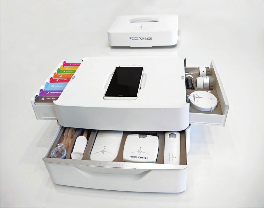
evenly distributed among genders and age ranges. The cho- Figure 1: XPRIZE DeepQ Tricorder. DeepQ consists of
sen diseases in this study were problem during pregnancy, four compartments. On the top is a mobile phone, which
prostate cancer venous insufficiency, actinic keratosis, lung runs a symptom checker. The drawer on the right-hand-side
cancer, skin cancer, chlamydia, and heart failure. As exam- contains optical sense. The drawer on the lower-front con-
ples of contextual influence, problem during pregnancy is tains vital sense and breath sense. The drawer on the left-
only associated with females, while prostate cancer is only hand-side contains blood/urine sense. The symptom checker
attributable to males. Venous insufficiency is unlikely to oc- guides a patient on which tests to conduct.
cur in children. We created another test set that only con-
tains the chosen context-influenced diseases and evaluated In our future work, we plan to further improve accuracy
the top-5 accuracy of our hierarchical models trained pre- by exploring three approaches.• Incorporating more information for diagnosis. As we Kohavi, R. 1996. Scaling up the accuracy of naive-Bayes
stated in the introduction section, without information classifiers: A decision-tree hybrid. In Proceedings of the
such as medical records, family history, and lab tests, Second International Conference on Knowledge Discovery
symptoms alone cannot achieve the optimal diagnosis ac- and Data Mining (KDD-96), Portland, Oregon, USA, 202–
curacy. Therefore, our first logical step is to incorporate 207.
more information into our model. We will also actively Kononenko, I. 1993. Inductive and Bayesian learning in
seek for or develop real-world datasets that we can use to medical diagnosis. Applied Artificial Intelligence 7(4):317–
conduct practical experiments. 337.
• Suggesting lab tests before diagnosis. We can use the Kononenko, I. 2001. Machine learning for medical diagno-
symptom checker as a tool to suggest collecting missing sis: history, state of the art and perspective. Artificial Intelli-
information when it can improve diagnosis accuracy. For gence in Medicine 23(1):89–109.
instance, when our model cannot decide between two dis- Ledley, R., and Lusted, L. 1959. Reasoning foundations
eases, it can suggest lab tests to provide missing infor- of medical diagnosis symbolic logic, probability, and value
mation for disambiguation. Once additional useful infor- theory aid our understanding of how physicians reason. Sci-
mation has been collected, we believe that diagnosis ac- ence 130(3366):9–21.
curacy will be further improved. In our XPRIZE DeepQ
Tricorder device (Chang et al. 2017), we indeed employ a Mnih, V.; Kavukcuoglu, K.; Silver, D.; Graves, A.;
symptom checker (see Figure 1) to suggest lab tests for a Antonoglou, I.; Wierstra, D.; and Riedmiller, M. A. 2013.
patient to conduct before a diagnosis. Playing Atari with deep reinforcement learning. CoRR
abs/1312.5602.
• Experimenting with other latent layers. In this paper, we
define our latent layer by separating diseases into dif- Mnih, V.; Kavukcuoglu, K.; Silver, D.; Rusu, A. A.; Ve-
ferent body parts. The user interface of our DeepQ Tri- ness, J.; Bellemare, M. G.; Graves, A.; Riedmiller, M.;
corder (Chang et al. 2017) benefits from this body-part- Fidjeland, A. K.; Ostrovski, G.; et al. 2015. Human-
grouping method. There are also other potential ways to level control through deep reinforcement learning. Nature
define our latent layer, such as grouping by systems (e.g., 518(7540):529–533.
digestive, nervous, circulatory, lymphatic urinary, repro- Nair, V., and Hinton, G. E. 2010. Rectified linear units im-
ductive, respiratory, and digestive). We believe that pur- prove restricted Boltzmann machines. In Proceedings of The
suing the best latent layer using a data-driven approach 27th International Conference on Machine Learning, 807–
could be a promising direction of research. 814.
National Institutes of Health. 2017. Unified medi-
Acknowledgements cal language system. https://www.nlm.nih.gov/
We would like to thank the following individuals for their research/umls/.
contributions. We thank Jocelyn Chang and Chun-Nan Chou Qualcomm. 2017. Xprize Tricorder Winning Teams.
for their help in proofreading the paper. We thank Chun-Yen http://tricorder.xprize.org/teams.
Chen, Ting-Wei Lin, Cheng-Lung Sung, Chia-Chin Tsao, Semigran, H. L.; Linder, J. A.; Gidengil, C.; and Mehrotra,
Kuan-Chieh Tung, Jui-Lin Wu, and Shang-Xuan Zou for A. 2015. Evaluation of symptom checkers for self diagnosis
their help in running the experiments of this paper. We also and triage: audit study. BMJ 351.
thank Ting-Jung Chang and Emily Chang for providing their
Sutton, R., and Barto, A. 1998. Reinforcement learning: An
medical knowledge.
introduction, volume 116. Cambridge Univ Press.
References Sutton, R. S.; Precup, D.; and Singh, S. 1999. Between
MDPs and semi-MDPs: A framework for temporal abstrac-
AHEAD Research Inc. 2017. SymCAT: Symptom-based, tion in reinforcement learning. Artificial intelligence 112(1-
computer assisted triage. http://www.symcat.com. 2):181–211.
Centers for Disease Control and Prevention. 2017. Ambula- Tang, K.-F.; Kao, H.-C.; Chou, C.-N.; and Chang, E. Y.
tory health care data. https://www.cdc.gov/nchs/ 2016. Inquire and diagnose: Neural symptom checking en-
ahcd/index.htm. semble using deep reinforcement learning. In NIPS Work-
Chang, E. Y.; Wu, M.-H.; Tang, K.-F.; Kao, H.-C.; and Chou, shop on Deep Reinforcement Learning.
C.-N. 2017. Artificial intelligence in XPRIZE DeepQ tri-
Wang, Z.; Schaul, T.; Hessel, M.; Hasselt, H.; Lanctot, M.;
corder. In MM Workshop on Multimedia and Health.
and Freitas, N. 2016. Dueling network architectures for deep
Hayashi, Y. 1991. A neural expert system with automated reinforcement learning. In Proceedings of The 33rd Interna-
extraction of fuzzy if-then rules and its application to med- tional Conference on Machine Learning, 1995–2003.
ical diagnosis. In Advances in Neural Information Process-
Zou, S.-X.; Chen, C.-Y.; Wu, J.-L.; Chou, C.-N.; Tsao, C.-
ing Systems 3. 578–584.
C.; Tung, K.-C.; Lin, T.-W.; Sung, C.-L.; and Chang, E. Y.
Johnson, A. E.; Pollard, T. J.; Shen, L.; wei H Lehman, 2017. Distributed training large-scale deep architectures. In
L.; Feng, M.; Ghassemi, M.; Moody, B.; Szolovits, P.; Celi, Proceedings of The 13th International Conference on Ad-
L. A.; and Mark, R. G. 2016. MIMIC-III, a freely accessible vanced Data Mining and Applications, 18–32.
critical care database. In Scientific data, volume 3.You can also read