Self-Supervised Learning of Audio-Visual Objects from Video
←
→
Page content transcription
If your browser does not render page correctly, please read the page content below
Self-Supervised Learning of
                                                        Audio-Visual Objects from Video

                                                               Triantafyllos Afouras1 , Andrew Owens2 ,
                                                             Joon Son Chung1,3 , and Andrew Zisserman1
                                                 1
                                                     University of Oxford, 2 University of Michigan, 3 Naver Corporation
arXiv:2008.04237v1 [cs.CV] 10 Aug 2020

                                               Abstract. Our objective is to transform a video into a set of discrete
                                               audio-visual objects using self-supervised learning. To this end, we in-
                                               troduce a model that uses attention to localize and group sound sources,
                                               and optical flow to aggregate information over time. We demonstrate the
                                               effectiveness of the audio-visual object embeddings that our model learns
                                               by using them for four downstream speech-oriented tasks: (a) multi-
                                               speaker sound source separation, (b) localizing and tracking speakers,
                                               (c) correcting misaligned audio-visual data, and (d) active speaker de-
                                               tection. Using our representation, these tasks can be solved entirely by
                                               training on unlabeled video, without the aid of object detectors. We
                                               also demonstrate the generality of our method by applying it to non-
                                               human speakers, including cartoons and puppets. Our model significantly
                                               outperforms other self-supervised approaches, and obtains performance
                                               competitive with methods that use supervised face detection.

                                                                                                                            (b) Localization and tracking
                                                                                                                            (c) Δt (AV synchronization)

                                                                 Audio-visual objects   (a) Multi-speaker source separation (d) Active speaker detection

                                         Fig. 1: We learn through self-supervision to represent a video as a set of discrete
                                         audio-visual objects. Our model groups a scene into object instances and repre-
                                         sents each one with a feature embedding. We use these embeddings for speech-
                                         oriented tasks that typically require object detectors: (a) multi-speaker source sep-
                                         aration, (b) speaker localization, (c) synchronizing misaligned audio and video,
                                         and (d) active speaker detection. Using our representation, these tasks can be
                                         solved without any labeled data, and on domains where off-the-shelf detectors are
                                         not available, such as cartoons and puppets. Please see our webpage for videos:
                                         http://www.robots.ox.ac.uk/∼vgg/research/avobjects.

                                         1   Introduction
                                         When humans organize the visual world into objects, hearing provides cues that
                                         affect the perceptual grouping process. We group different image regions together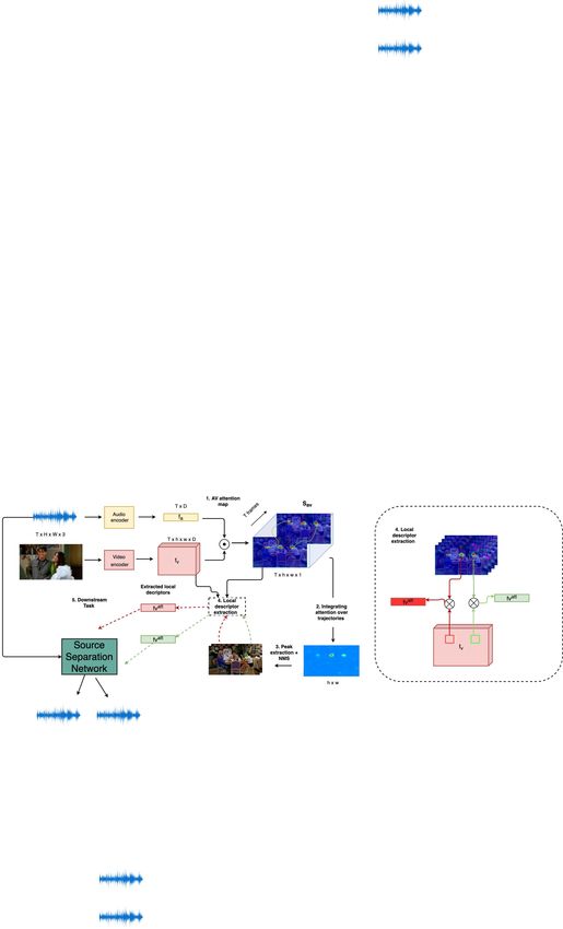
2       T. Afouras et al.

not only because they look alike, or move together, but also because grouping
them together helps us explain the causes of co-occurring audio signals.
    In this paper, our objective is to replicate this organizational capability, by
designing a model that can ingest raw video and transform it into a set of discrete
audio-visual objects. The network is trained using only self-supervised learning
from audio-visual cues. We demonstrate this capability on videos containing
talking heads.
    This organizational task must overcome a number of challenges if it is to
be applicable to raw videos in the wild: (i) there are potentially many visually
similar sound generating objects in the scene (multiple heads in our case), and
the model must correctly attribute the sound to the actual sound source; (ii)
these objects may move over time; and (iii) there can be multiple other objects
in the scene (clutter) as well.
   To address these challenges, we build upon recent works on self-supervised
audio-visual localization. These include video methods that find motions tem-
porally synchronized with audio onsets [13, 40, 46], and single-frame meth-
ods [6, 31, 48, 54] that find regions that are likely to co-occur with the audio.
However, their output is a typically a “heat map” that indicates whether a given
pixel is likely (or unlikely) to be attributed to the audio; they do not group a
scene into discrete objects; and, if only using semantic correspondence, then they
cannot distinguish which, of several, object instances is making a sound.
    Our first contribution is to propose a network that addresses all three of
these challenges; it is able to use synchronization cues to detect sound sources,
group them into distinct instances, and track them over time as they move. Our
second contribution is to demonstrate that object embeddings obtained from
this network facilitate a number of audio-visual downstream tasks that have
previously required hand-engineered supervised pipelines.
    As illustrated in Figure 1, we demonstrate that the embeddings enable: (a)
multi-speaker sound source separation [2, 19]; (b) detecting and tracking talking
heads; (c) aligning misaligned recordings [12, 14]; and (d) detecting active speak-
ers, i.e. identifying which speaker is talking [13, 52]. In each case, we significantly
outperform other self-supervised localization methods, and obtain comparable
(and in some cases better) performance to prior methods that are trained using
stronger supervision, despite the fact that we learn to perform them entirely
from a raw audio-visual signal.
    The trained model, which we call the Look Who’s Talking Network (LWTNet),
is essentially “plug and play” in that, once trained on unlabeled data (without
preprocessing), it can be applied directly to other video material. It can easily be
fine-tuned for other audio-visual domains: we demonstrate this functionality on
active speaker detection for non-human speakers, such as animated characters in
The Simpsons and puppets in Sesame Street. This demonstrates the generality
of the model and learning framework, since this is a domain where off-the-shelf
supervised methods, such as methods that use face detectors, cannot transfer
without additional labeling.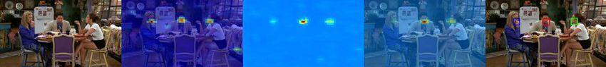
Self-Supervised Learning of Audio-Visual Objects from Video         3

2   Related work
Sound source localization. Our task is closely related to the sound source
localization problem, i.e. finding the location in a video that is the source of a
sound. Early work performed localization [7, 21, 34, 39] and segmentation [37]
by doing inference on simple probabilistic models, such as methods based on
canonical correlation analysis.
    Recent efforts learn audio and video representations using self-supervised
learning [13, 40, 46] with synchronization as the proxy task: the network has to
predict whether video and audio are temporally aligned (or synthetically shifted).
Owens and Efros [46] show via heat-map visualizations that their network often
attends to sound sources, but do not quantitatively evaluate their model. Recent
work [38] added an attention mechanism to this model. Other work has detected
sound-making objects using correspondence cues [6, 31, 35, 36, 48, 50, 54, 56],
e.g. by training a model to predict whether audio and a single video frame come
from the same (or different) videos. Since these models do not use motion and are
trained only to find the correspondence between object appearance and sound,
they would not be able to identify which of several objects of the same category
is the actual source of a sound. In contrast, our goal is to obtain discrete audio-
visual objects from a scene, even when they bellong to the same category (e.g.
multiple talking heads). In a related line of work, [24] distill visual object detec-
tors into an audio model using stereo sound, while [26] use spatial information
in a scene to convert mono sound to stereo.
Active speaker detection (ASD). Early work on active speaker detection
trained simple classifiers on hand-crafted feature sets [15]. Later, Chung and
Zisserman [13] used synchronization cues to solve the active speaker detection
problem. They used a hand-engineered face detection and tracking pipeline to
select candidate speakers, and ran their model only on cropped faces. In con-
trast, our model learns to do ASD entirely from unlabeled data. Chung et al.[11]
extended the pipeline by enrolling speaker models from visible speaking seg-
ments. Recently, Roth et al. [52] proposed an active speaker detection dataset
and evaluated a variety of supervised methods for it.
Source separation.         In recent years, researchers have proposed a variety of
methods for separating the voices of multiple speakers in a scene [2, 19, 22, 46].
These methods either only handle a single on-screen speaker [46] or use hand-
engineered, supervised face detection pipelines. Afouras et al. [2] and Ephrat et
al. [19], for example, detect and track faces and extract visual representations
using off-the-shelf packages. In contrast, we use our model to separate multiple
speakers entirely via self-supervision.
    Other recent work has explored separating the sounds of musical instruments
and other sound-making objects. Gao et al. [25, 27] use semantic object detectors
trained on instrument categories, while [53, 60] do not explicitly group a scene
into objects and instead either pool the visual features or produce a per-pixel
map that associates each pixel with a separated audio source. Recently, [59]
added motion information from optical flow. We, too, use flow in our model, but
4          T. Afouras et al.

                         1. Audio-visual attention map               2. Integrate attention over time   4. Local descriptor
                                                                                                            extraction
                                                    T×D                            Sav
                            Audio
                           encoder                    fa
                                                   T×hxwxD

                            Video                      fv
                           encoder
                                                                                                         fvatt       fvatt
                                                                           3. Find peaks
                                                                              & NMS
     Local descriptors                              Audio-visual objects

           fvatt                                                                                                 x
                          4. Local descriptor                                                                          fv
                         & trajectory extraction
           fvatt
                                                                                  hxw

                                          5. Downstream tasks
                                                                                                        …
     Active                         Correcting                         Δt             Multi-speaker
    speaker?                       misalignment                                     source separation

Fig. 2: The Look Who’s Talking Network (LWTNet): (1) Computes an audio-
visual attention map Sav by solving a synchronization task, (2) accumulates attention
over time, (3) selects audio-visual objects by computing the N highest peaks with non-
maximum suppression (NMS) from the accumulated attention map, each corresponding
to a trajectory of the pixel over time; (4) for every audio-visual object, it extracts
embedding vectors from a spatial window ρ, using the local attention map Sav to select
visual features, and (5) provides the audio-visual objects as inputs to downstream tasks.

instead of using it as a cue for motion, we use it to integrate information from
moving objects over time [23, 49] in order to track them. In concurrent work [36]
propose a model that groups and separates sound sources by clustering audio
and video embeddings.
Representation learning.           In recent years, researchers have proposed a
variety of self-supervised learning methods for learning representations from im-
ages [10, 17, 32, 33, 42, 45, 57, 58], videos [29, 30] and multimodal data [5, 40,
43, 47, 48]. Often the representation learned by these methods is a feature set
(e.g., CNN weights) that can be adapted to downstream tasks by fine-tuning.
By contrast, we learn an additional attention mechanism that can be used to
group discrete objects of interest for downstream speech tasks.

3       From unlabeled video to audio-visual objects
Given a video, the function of our model is to detect and track (possibly several)
audio-visual objects, and extract embeddings for each of them. We represent
an audio-visual object as the trajectory of a potential sound source through
space and time, which in the domain that we experiment on is often the track
of a “talking head”. Having obtained these trajectories, we use them to extract
embeddings that can be then used for downstream tasks.
    In more detail, our model uses a bottom-up grouping procedure to propose
discrete audio-visual objects from raw video. It first estimates local (per-pixel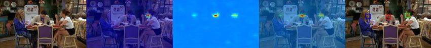
Self-Supervised Learning of Audio-Visual Objects from Video        5

and per-frame) synchronization evidence, using a network design that is more
fine-grained in space and time than prior models. It then aggregates this evi-
dence over time via optical flow, thereby allowing the model to obtain robustness
to motions, and groups the aggregated attention into sound sources by detect-
ing local maxima. The model represents each object as a separate embedding,
temporal track, and attention map that can be adjusted in downstream tasks.
    We will now give an overview of the model, which is shown in Figure 2,
followed by the learning framework which uses self-supervision based on syn-
chronization. For architecture details refer to Appendix D.

3.1   Estimating audio-visual attention

Before we group a scene into sound sources, we estimate a per-pixel attention
map that picks out the regions of a video whose motions have a high degree
of synchronization with the audio. We propose an attention mechanism that
provides highly localized spatio-temporal attention, and which is sensitive to
speaker motion. As in [6, 31], we estimate audio-visual attention via a multimodal
embedding (Figure 2, step 1). We learn vector embeddings for each audio clip
and embedding vectors for each pixel, such that if a pixel’s vector has a high dot
product with that of the audio, then it is likely to belong to that sound source.
For this, we use a two-stream architecture similar to those in other sound-source
localization work [6, 31, 54], with a network backbone similar to [11]. We now
describe this model in more detail.

Video encoder. Our video feature encoder is a spatio-temporal VGG-M [9]
with a 3D convolutional layer first, followed by a stack of 2D convolutions. Given
a T × H × W × 3 input RGB video, it extracts a video embedding map fv (x, y, t)
with dimensions T × h × w × D.

Audio encoder.      The audio encoder is a VGG-M network operating on log-
mel spectrograms, treated as single-channel images. Given an audio segment, it
extracts a D-dimensional embedding fa (t) for every corresponding video frame t.

Computing fine-grained attention maps.             For each space-time pixel, we
ask: how correlated is it with the events in the audio? To estimate this, we
measure the similarity between the audio and visual features at every spatial
location. For every space-time feature vector fv (x, y, t), we compute the cosine
similarity with the audio feature vector fa (t):

                          Sav (x, y, t) = fv (x, y, t)·fa (t),                  (1)

where we first l2 normalize both features. We refer to the result, Sav (x, y, t), as
the audio-visual attention map.

3.2   Extracting audio-visual objects

Given the audio-visual evidence, we parse a video into object representations.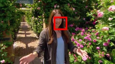
6       T. Afouras et al.

                                   Input                                     Aggregated
                                                                           attention + NMS

                            Per-frame attention                          Audio-visual objects

Fig. 3: Intermediate representations from our model. We show the per-frame
                                                      tr
attention maps Sav (t), the aggregated attention map Sav and the two highest scoring
extracted audio-visual objects. We show the audio-visual objects for a single frame,
with a square of constant width.

Integrating evidence over time. Audio-visual objects may only intermit-
tently make sounds. Therefore, we need to integrate sparse attention evidence
over time. We also need to group and track sound sources between frames, while
accounting for camera and object motion. To make our model more robust to
these motions, we aggregate information over time using optical flow (Figure 2,
step 2). We extract dense optical flow for every frame, chain the flow values
together to obtain long-range tracks, and average the attention scores over these
tracks. Specifically, if T (x, y, t) is the tracked location of pixel (x, y) from frame
1 to the later frame t, we compute the score:
                                              T
                         tr                1X
                        Sav (x, y) =             Sav (T (x, y, t), t),                  (2)
                                           T t=1

where we perform the sampling using bilinear interpolation. The result is a 2D
map containing a score for the future trajectory of every pixel of the initial frame
through time. Note that any tracking method can be used in place of optical flow
(e.g. with explicit occlusion handling); we use optical flow for simplicity.
Grouping a scene into instances. To obtain discrete audio-visual objects,
we detect spatial local maxima (peaks) on the temporally aggregated synchro-
nization maps, and apply non-maximum suppression (NMS). More specifically,
                                                               tr
we find peaks in the time-averaged synchronization map, Sav       (x, y), and sort
them in decreasing order; we then choose the peaks greedily, each time suppress-
ing the ones that are within a ρ × ρ box. The selected peaks can be now viewed
as distinct audio-visual objects. Examples of the intermediate representations
extracted at the steps described so far are shown in Figure 3.
Extracting object embeddings.              Now that the sound sources have been
grouped into distinct audio-visual objects, we can extract feature embeddings
for each one of them that we can use in downstream tasks. Before extracting
these features, we locate the position of the sound source in each frame. A simple
strategy for this would be to follow the object’s optical flow track throughout
the video. However, these tracks are imprecise and may not correspond precisely
to the location of the sound source. Therefore, we “snap” to the track location
to the nearest peak in the attention map. More specifically, in frame t, we search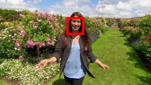
Self-Supervised Learning of Audio-Visual Objects from Video        7

in an area of ρ×ρ centered on the tracked location T (x, y, t), and select the pixel
location with largest attention value. Then, having tracked the sound source in
each frame, we select the corresponding spatial feature vector from the visual
feature map fv (Figure 2, step 4). These per-frame embedding features, fvatt (t),
can then be used to solve downstream tasks (Section 4). One can equivalently
view this procedure as an audio-visual attention mechanism that operates on fv .

3.3   Learning the attention map
Training our model amounts to learning the attention map Sav on which the
audio-visual objects are subsequently extracted. We obtain this map by solving
a self-supervised audio-visual synchronization task [13, 40, 46]: we encourage the
embedding at each pixel to be correlated with the true audio and uncorrelated
with shifted versions of it. We estimate the synchronization evidence for each
frame by aggregating the per-pixel synchronization scores. Following common
practice in multiple instance learning [6], we measure the per-frame evidence by
the maximum spatial response:
                               att
                              Sav  (t) = max Sav (x, y, t).                     (3)
                                           x,y

    We maximize the similarity between a video frame’s true audio track while
minimizing that of N shifted (i.e. misaligned) versions of the audio. Given visual
features fv and true audio ai , we sample N other audio segments from the same
video clip: a1 , a2 , ..., aN , and minimize the contrastive loss [14, 45]:
                                                att
                                          exp(Sav   (v, ai ))
                 L = − log                      PN                         .     (4)
                                  att
                             exp(Sav (v, ai )) + j=1 exp(Sav  att (v, a ))
                                                                       j

For the negative examples, we select all audio features (except for the true ex-
ample) in a temporal window centered on the video frame.
   In addition to the synchronization task, we also consider the correspondence
task of Arandjelović and Zisserman [6], which chooses negatives audio samples
from random video clips. Since this problem can be solved with even a single
frame, it results in a model that is less sensitive to motion.

4     Applications of audio-visual object embeddings
Having grouped the video into audio-visual objects, we can use the learned
representation to perform a variety of tasks that, in previous work, often required
face detection: 1) speaker localization, 2) audio-visual synchronization, 3) active
speaker detection, and 4) audio-visual multi-speaker source separation. We also
show the generality of our method by applying it to non-human speakers, such
as puppets and animated characters.

4.1   Audio-visual object detection and tracking
We can use our model for spatially localizing speakers. To do this, we use the
tracked location of an audio-visual object in each frame.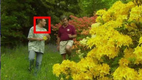
8 T. Afouras et al.
Separation
fvatt
network
Separation
fvatt
network
Separation
fvatt
network
Input video + audio Audio-visual objects Separated sound
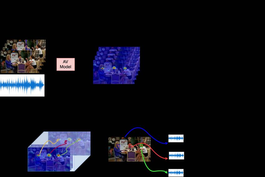
Fig. 4: Multi-speaker separation. We isolate the sound of each speaker’s voice by
combining our audio-visual objects with a network similar to [2]. Given a spectrogram
of a noisy sound mixture, the network isolates the voice of each speaker, using the
visual features provided by their audio-visual object.
4.2 Active speaker detection
For every frame in our video, our model can locate potential speakers and decide
whether or not they are speaking. In our setting, this can be viewed as decid-
ing whether an audio-visual object has strong evidence of synchronization in a
given frame. For every tracked audio-visual object, we extract the visual features
fvatt (t) (Sec. 3.2) for each frame t. We then obtain a score that indicates how
strong the audio-visual correlation for frame t is, by computing the dot product:
fvatt (t)·fa (t). Following previous work [13], we threshold the result to make a
binary decision (active speaker or not).
4.3 Multi-speaker source separation
Our audio-visual objects can also be used for separating the voices of speakers
in a video. We consider the multi-speaker separation problem [2, 19]: given a
video with multiple people speaking on-screen (e.g., a television debate show),
we isolate the sound of each speaker’s voice from the audio stream. We note that
this problem is distinct from on/off-screen audio separation [46], which requires
only a single speaker to be on-screen.
We train an additional network that, given a waveform containing an audio
mixture and an audio-visual object, isolates the speaker’s voice (Figure 4, full
details in Appendix D). We use an architecture that is similar to [2], but con-
ditions on our self-supervised representations instead of detections from a face
detector. More specifically, the method of [2] runs a face detection and tracking
system on a video, computes CNN features on each crop, and then feeds those
to a source separation network. We, instead, simply provide the same separation
network with the embedding features fvatt (t).
4.4 Correcting audio-visual misalignment
We can also use our model to correct misaligned audio-visual data — a problem
that often occurs in the recording and television broadcast process. We follow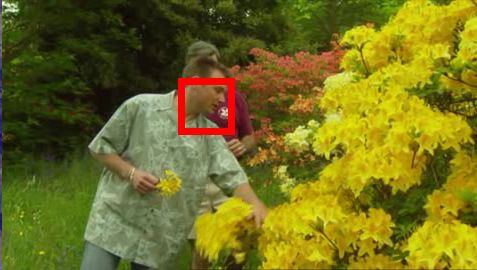
Self-Supervised Learning of Audio-Visual Objects from Video       9

the problem formulation proposed by Chung and Zisserman [13]. While this is
a problem that is typically solved using supervised face detection [13, 14], we
instead tackle it with our learned model. During inference, we are given a video
with unsynchronized audio and video tracks, and we shift the audio to discover
           ˆ that maximizes the audio-visual evidence:
the offset ∆t
                                           T
                            ˆ = arg max 1
                                          X    att
                            ∆t                S∆t  (t),                         (5)
                                   ∆t   T t=1
        att
where S∆t   (t) is the synchronization score of frame t after shifting the audio by
∆t. Note that this can be estimated efficiently by simply recomputing the dot
products in Equation 1.
   In addition to treating this alignment procedure as a stand-alone application,
we also use it as a preprocessing step for our other applications (a common
practice in other speech analysis work [2]). When given a test video, we first
compute the optimal offset ∆t, ˆ and use it to shift the audio accordingly. We
then recompute Sav (t) from the synchronized embeddings.

5     Experiments
5.1   Datasets
Human speech.           We evaluate our model on the Lip Reading Sentences
(LRS2 and LRS3) datasets and the Columbia active speaker dataset. LRS2 [1]
and LRS3 [3] are audio-visual speech datasets containing 224 and 475 hours
of videos respectively, along with ground truth face tracks of the speakers. The
Columbia dataset [8] contains footage from an 86-minute panel discussion, where
multiple individuals take turns in speaking, and contains approximate bounding
boxes and active speaker labels, i.e. whether a visible face is speaking at a
given point in time. All datasets provide (pseudo-)ground truth bounding boxes
obtained via face detection, which we use for evaluation.
    We resample all videos to a resolution of H × W = 270 × 480 pixels before
feeding them to our model, which outputs h × w = 18 × 31 attention maps. We
train and evaluate all models (except for those with non-human speakers) on
LRS2, and use LRS3 only for evaluation.
Non-human speakers            To evaluate our method on non-human speakers,
we collected television footage from The Simpsons and Sesame Street shows
(Table 3a). We trained on the raw footage without performing any preprocessing,
except for splitting the videos into scenes. For testing, we collected ASD and
speaker localization labels, using the VIA tool [18]: we asked human annotators
to label frames that they believed to contain an active speaker and to localize
them. Videos were annotated sparsely with only a few frames per video clip.
For every dataset, we create two test sets. In the single-head set, the clips are
constrained to contain a single active speaker, with no other faces. The second
test subset, multi-head, may contain multiple heads — talking or not — and also
a variety of cases with no relevant speech (non-talking heads, background, title
sequences etc.). We summarize the statistics of the test sets in Table 3a. For full
details refer to Appendix C.
10      T. Afouras et al.

                                    AVOL-net [6]

                                     Our model
Fig. 5: Talking head detection and tracking on LRS3 datasets. For each of
the 4 examples, we show the audio-visual attention score on every spatial location for
the depicted frame, and a bounding box centered on the largest value, indicating the
speaker location. Please see our webpage for video results.

5.2   Training details

Fig. 6: Handling motion: Talking head detection and tracking on continuous scenes
from the validation set of LRS2. Despite the significant movement of the speakers and
the camera, our method accurately tracks them.

Audio-visual object detection training. To make training easier, we fol-
low [40] and use a simple learning curriculum. At the beginning of training, we
sample negatives from random video clips, then switch to shifted audio tracks
later in training. To speed up training, we also begin by taking the mean dot
product (Eq. 3), and then switch to the maximum. We set ρ to 100 pixels.
Source separation training Training takes place in two steps: we first train
our model to produce audio-visual objects by solving a synchronization problem.
Then, we train the multi-speaker separation network on top of these learned rep-
resentations. We follow previous work [2, 19] and use a mix-and-separate learning
procedure. We create synthetic videos containing multiple talking speakers by
1) selecting two or three videos at random from the training set, depending on
the experiment, 2) summing their waveforms together, and 3) vertically concate-
nating the video frames together. The model is then tasked with extracting a
number of talking heads equal to the number of mixed videos and predicting an
original corresponding waveform for each.
Non-human model training              We fine-tune the best model from LRS2
separately on each of the two datasets with non-human speakers. The lip motion
for non-human speakers, such as the motion of a puppet’s mouth, is only loosely
correlated with speech, suggesting that there is less of an advantage to obtaining
Self-Supervised Learning of Audio-Visual Objects from Video 11
Fig. 7: Active speaker detection on the Columbia dataset, and an example from
the Friends TV show. We show active speakers in blue and inactive speakers in red.
The corresponding detection scores are noted above the boxes (the threshold has been
subtracted so that positive scores indicate active speakers).
Fig. 8: Active speaker detection for non-human speakers. We show the top 2
highest-scoring audio-visual objects in each scene, along with the aggregated attention
map. Please see our webpage for video results.
our negative examples from temporally shifted audio. We therefore sample our
negative audio examples from other video clips rather than from misaligned
audio (Section 3.3) when computing attention maps, but keep the rest of the
architecture the same.
5.3 Results
1. Talking head detection and tracking. We evaluate how well our model
is able to localize speakers, i.e. talking heads (Table 1a). First, we evaluate two
simple baselines: the random one, which selects a random pixel in each frame and
the center one, which always selects the center pixel. Next, we compared with
two recent sound source localization methods: Owens and Efros [46] and AVOL-
net [6]. Since these methods require input videos that are longer than most of the
videos in the test set of LRS2, we only evaluate them on LRS3. We also perform
several ablations of our model: To evaluate the benefit of integrating the audio-
visual evidence over flow trajectories, we create a variation of our model called
tr
No flow that, instead, computes the attention Sav by globally pooling over time
throughout the video. Finally, we also consider a variation of this model that
uses a larger NMS window (ρ = 150).
We found that our method obtains very high accuracy, and that it signifi-
cantly outperforms all other methods. AVOL-net solves a correspondence task
that doesn’t require motion information, and uses a single video frame as input.12 T. Afouras et al.
Method LRS2 LRS3
Random 2.8% 2.9% Method Speaker
Center 23.9% 25.9% Bell Boll Lieb Long Sick Avg.
Owens & Efros [46] - 24.8%
Chakravarty [8] 82.9 65.8 73.6 86.9 81.8 80.2
AVOL-net [6] - 58.1%
No flow 98.4% 94.2% Shahid [55] 87.3 96.4 92.2 83.0 87.2 89.2
No flow + large NMS 98.8% 97.2% SyncNet [13] 93.7 83.4 86.8 97.7 86.1 89.5
Full model 99.6% 99.7% Ours 92.6 82.4 88.7 94.4 95.9 90.8
Table 1(a): Talking head detec- Table 1(b): Active speaker detection accu-
tion and tracking accuracy. A racy on the Columbia dataset [8]. F1 Scores
detection is considered correct if it (%) for each speaker, and the overall average.
lies within the true bounding box.
Consequently, it does not take advantage of informative motion, such as moving
lips. As can be seen in Figure 5, the localization maps produced by AVOL-net [6]
are less precise, as it only loosely associates appearance of a person to speech,
and won’t consistently focus on the same region. Owens and Efros [46], by con-
trast, has a large temporal receptive field, which results in temporally imprecise
predictions, causing very large errors when the subjects are moving. The No
flow baseline fails to track the talking head well outside the NMS area, and
its accuracy is consequently lower on LRS3. Enlarging the NMS window par-
tially alleviates this issue, but the accuracy is still lower than that of our model.
We note that the LRS2 test set contains very short clips (usually 1-2 seconds
long) with predominantly static speakers, which explains why using flow does
not provide an advantage.
We show some challenging examples with significant speaker and camera
motion in Figure 6. Refer to Appendix A for further analysis on robustness to
camera and speaker motion.
2. Active speaker detection. Next, we ask how well our model can determine
which speaker is talking. Following previous work that uses supervised face de-
tection [13, 55], we evaluate our method on the Columbia dataset [8]. For each
video clip, we extract 5 audio-visual objects (an upper bound on the number of
speakers), each of which has an ASD score indicating the likelihood that it is a
sound source (Section 4.2). We then associate each ground truth bounding box
with the audio-visual object whose trajectory follows it the closest. For compari-
son with existing work, we report the F1 measure (the standard for this dataset)
per individual speaker as well as averaged over all speakers. For calculating the
F1 we set the ASD threshold to the one that yields the Equal Error Rate (EER)
for the pretext task on the LRS2 validation set. As shown in Table 1b, our model
outperforms all previously reported results on this dataset, even though (unlike
other methods) it does not use labeled face bounding boxes for training.
3. Multi-speaker source separation. To evaluate our model on speaker
separation, we follow the protocol of [2]. We create synthetic examples from the
test set of LRS2, using only videos that are between 2 − 5 seconds long, and
evaluate performance using Signal-to-Distortion-Ratio (SDR) [20] and Percep-Self-Supervised Learning of Audio-Visual Objects from Video 13
SDR PESQ WER %
Input frames
Method \ # Spk. 2 3 2 3 2 3
Mixed input -0.3 -3.4 1.7 1.5 91.0 97.2 Method 5 7 9 11 13 15
Conv.-Sync [2] 11.3 7.5 3.0 2.5 30.3 43.5
SyncNet [13] 75.8 82.3 87.6 91.8 94.5 96.1
Frozen 10.7 7.0 3.0 2.5 30.7 44.2
Ours Oracle-BB 10.8 7.1 2.9 2.5 30.9 44.9 PM [14] 88.1 93.8 96.4 97.9 98.7 99.1
Small-NMS 10.6 6.8 3.0 2.5 31.2 44.7
Full 10.8 7.2 3.0 2.6 30.4 42.0 Ours 78.8 87.1 92.1 94.8 96.3 97.3
Table 2(a): Source separation on LRS2. Table 2(b): Audio-visual synchro-
#Spk indicates the number of speakers. The nization accuracy (%) evaluation for
WER on the ground truth signal is 20.0%. a given number of input frames.
tual Evaluation of Speech Quality (PESQ, varies between 0 and 4.5) [51] (higher
is better for both). We also assess the intelligibility of the output by computing
the Word Error Rate (WER, lower is better) between the transcriptions obtained
with the Google Cloud speech recognition system. Following [3], we train and
evaluate separate models for 2 and 3 speakers, though we note that if the number
of speakers were unknown, it could be estimated using active speaker detection.
For comparison, we implement the model of Afouras et al. [2], and train it on
the same data. For extracting visual features to serve as its input, we use a state-
of-the-art audio-visual synchronization model [14], rather than the lip-reading
features from Afouras et al. [4]. We refer to this model as Conversation-Sync.
This model uses bounding boxes from a well-engineered face detection system,
and thus represents an approximate upper limit on the performance of our self-
supervised model. Our main model for this experiment is trained end-to-end and
uses ρ = 150. We also performed a number of ablations: a model that freezes the
pretrained audio-visual features and a model with a smaller ρ = 100.
We observed (Table 2a) that our self-supervised model obtains results close
to those of [2], which is based on supervised face detection. We also asked how
much error is introduced by lack of face detection. In this direction we extract
the local visual descriptors using tracks obtained with face detectors instead of
our audio-visual object tracks. This model, Oracle-BB, obtains results similar to
ours, suggesting that the quality of our face localization is high.
4. Correcting misaligned visual and audio data. We use the same
metric as [14] to evaluate on LRS2. The task is to determine the correct audio-
to-visual offset within a ±15 frame window. An offset is considered correct if it
is within 1 video frame from the ground truth. The distances are averaged over
5 to 15 frames. We compare our method to two state-of-the-art synchronization
methods: SyncNet [13] and the state-of-the-art Perfect Match [14]. We note that
[14] represents an approximate upper limit to what we would expect our method
to achieve, since we are using a similar network and training objective; the major
difference is that we use our audio-visual objects instead of image crops from a
face detector. The results (Table 2b) show that our self-supervised model obtains
comparable accuracy to these supervised methods.14 T. Afouras et al.
Loc. Acc ASD AP
Single-head Single-head Multi-head
Source Type Clips Frames Method Simp. Ses. Simp. Ses. Simp. Ses.
The Simpsons S 41 87 Random 8.7 16.0 - - - -
The Simpsons M 582 251 Center 62.0 80.1 - - - -
RetinaFace RN 47.7 61.2 40.0 46.8 - -
Sesame Street S 57 120 RetinaFace MN 72.1 70.2 60.4 52.4 - -
Sesame Street M 143 424 Ours 98.8 81.0 98.7 72.2 85.5 55.6
Table 3(a): Label statistics for Table 3(b): Non-human speaker evaluation
non-human test sets. S is single for ASD and localization tasks on Simpsons and
head and M multi-head. Sesame Street. MN: MobileNet; RN: ResNet50.
5. Generalization to non-human speakers. We evaluate the LWTNet
model’s generalization to non-human speakers using the Simpsons and Sesame
Street datasets described in Section 5.1. The results of our evaluation are sum-
marized in Table 3b. Since supervised speech analysis methods are often based
on face detection systems, we compare our method’s performance to off-the-
shelf face detectors, using the single-head subset. As a face detector baseline, we
use the state-of-the-art RetinaFace [16] detector, with both the MobileNet and
ResNet-50 backbones. We report localization accuracy (as in Table 1a) and Av-
erage Precision (AP). It is clear that our model outperforms the face detectors
in both localization and retrieval performance for both datasets.
The second evaluation setting is detecting active speakers in videos from
the multi-head test set. As expected, our model’s performance decreases in this
more challenging scenario; however, the AP for both datasets indicates that our
method can be useful for retrieving the speaker in this entirely new domain. We
show qualitative examples of ASD on the multi-head test sets in Figure 8.
6 Conclusion
In this paper, we have proposed a unified model that learns from raw video to
detect and track speakers. The embeddings learned by the model are effective
for many downstream speech analysis tasks, such as source separation and active
speaker detection, that in previous work required supervised face detection.
We see our work opening two new directions. The first one is in extending
our object embeddings to other audio-visual speaker tasks, such as diarizing con-
versations [11, 28], and face/head detection. The second one is in self-supervised
representation learning. We have presented a framework that is well-suited to
speech tasks but could also have potential in different domains, such as the anal-
ysis of music and ambient sounds. For code and models, please see our webpage.
Acknowledgements. We thank V. Kalogeiton for generous help with the anno-
tations and the Friends videos, A. A. Efros for helpful discussions, L. Momeni,
T. Han and Q. Pleple for proofreading, A. Dutta for help with VIA, and A.
Thandavan for infrastructure support. This work is funded by the UK EPSRC
CDT in AIMS, DARPA Medifor, and a Google-DeepMind Graduate Scholarship.Bibliography
[1] Afouras, T., Chung, J.S., Senior, A., Vinyals, O., Zisserman, A.: Deep audio-
visual speech recognition. IEEE PAMI (2019) 9
[2] Afouras, T., Chung, J.S., Zisserman, A.: The conversation: Deep audio-
visual speech enhancement. In: INTERSPEECH (2018) 2, 3, 8, 9, 10, 12,
13, 23
[3] Afouras, T., Chung, J.S., Zisserman, A.: LRS3-TED: a large-scale dataset
for visual speech recognition. In: arXiv preprint arXiv:1809.00496 (2018) 9,
13, 21
[4] Afouras, T., Chung, J.S., Zisserman, A.: My lips are concealed: Audio-visual
speech enhancement through obstructions. In: INTERSPEECH (2019) 13,
23
[5] Arandjelović, R., Zisserman, A.: Look, listen and learn. In: Proc. ICCV
(2017) 4
[6] Arandjelovic, R., Zisserman, A.: Objects that sound. In: Proc. ECCV (2017)
2, 3, 5, 7, 10, 11, 12
[7] Barzelay, Z., Schechner, Y.Y.: Harmony in motion. In: 2007 IEEE Confer-
ence on Computer Vision and Pattern Recognition (2007) 3
[8] Chakravarty, P., Tuytelaars, T.: Cross-modal supervision for learning active
speaker detection in video. In: Proc. ECCV (2016) 9, 12
[9] Chatfield, K., Simonyan, K., Vedaldi, A., Zisserman, A.: Return of the
devil in the details: Delving deep into convolutional nets. arXiv preprint
arXiv:1405.3531 (2014) 5
[10] Chen, T., Kornblith, S., Norouzi, M., Hinton, G.: A simple framework for
contrastive learning of visual representations. ICML (2020) 4
[11] Chung, J.S., Lee, B.J., Han, I.: Who said that?: Audio-visual speaker diari-
sation of real-world meetings. In: Interspeech (2019) 3, 5, 14
[12] Chung, J.S., Nagrani, A., Zisserman, A.: VoxCeleb2: Deep speaker recogni-
tion. In: INTERSPEECH (2018) 2
[13] Chung, J.S., Zisserman, A.: Out of time: automated lip sync in the wild.
In: Workshop on Multi-view Lip-reading, ACCV (2016) 2, 3, 7, 8, 9, 12, 13,
21, 22
[14] Chung, S.W., Chung, J.S., Kang, H.G.: Perfect match: Improved cross-
modal embeddings for audio-visual synchronisation. In: Proc. ICASSP. pp.
3965–3969. IEEE (2019) 2, 7, 9, 13
[15] Cutler, R., Davis, L.: Look who’s talking: Speaker detection using video and
audio correlation. In: 2000 IEEE International Conference on Multimedia
and Expo. ICME2000. Proceedings. Latest Advances in the Fast Changing
World of Multimedia (Cat. No. 00TH8532). vol. 3, pp. 1589–1592. IEEE
(2000) 3
[16] Deng, J., Guo, J., Yuxiang, Z., Yu, J., Kotsia, I., Zafeiriou, S.: Retinaface:
Single-stage dense face localisation in the wild. In: arxiv (2019) 14, 2116 T. Afouras et al.
[17] Doersch, C., Gupta, A., Efros, A.A.: Unsupervised visual representation
learning by context prediction. In: Proc. ICCV. pp. 1422–1430 (2015) 4
[18] Dutta, A., Zisserman, A.: The VIA annotation software for images, audio
and video. In: Proceedings of the 27th ACM International Conference on
Multimedia. MM ’19, ACM, New York, NY, USA (2019) 9, 20
[19] Ephrat, A., Mosseri, I., Lang, O., Dekel, T., Wilson, K., Hassidim, A.,
Freeman, W.T., Rubinstein, M.: Looking to listen at the cocktail party: a
speaker-independent audio-visual model for speech separation. ACM Trans-
actions on Graphics (TOG) 37(4), 112 (2018) 2, 3, 8, 10, 21
[20] Févotte, C., Gribonval, R., Vincent, E.: BSS EVAL toolbox user guide.
IRISA Technical Report 1706. http://www.irisa.fr/metiss/bss eval/. (2005)
12
[21] Fisher III, J.W., Darrell, T., Freeman, W.T., Viola, P.A.: Learning joint sta-
tistical models for audio-visual fusion and segregation. In: NeurIPS (2000)
3
[22] Gabbay, A., Ephrat, A., Halperin, T., Peleg, S.: Seeing through noise: Vi-
sually driven speaker separation and enhancement. In: Proc. ICASSP. pp.
3051–3055. IEEE (2018) 3
[23] Gadde, R., Jampani, V., Gehler, P.V.: Semantic video cnns through repre-
sentation warping. In: Proc. ICCV. pp. 4463–4472 (2017) 4
[24] Gan, C., Zhao, H., Chen, P., Cox, D., Torralba, A.: Self-supervised moving
vehicle tracking with stereo sound. In: Proceedings of the IEEE Interna-
tional Conference on Computer Vision. pp. 7053–7062 (2019) 3
[25] Gao, R., Feris, R.S., Grauman, K.: Learning to separate object sounds by
watching unlabeled video. In: Proc. ECCV (2018) 3
[26] Gao, R., Grauman, K.: 2.5d visual sound. In: CVPR (2019) 3
[27] Gao, R., Grauman, K.: Co-separating sounds of visual objects. arXiv
preprint arXiv:1904.07750 (2019) 3
[28] Gebru, I.D., Ba, S., Li, X., Horaud, R.: Audio-visual speaker diarization
based on spatiotemporal bayesian fusion. IEEE PAMI (2017) 14
[29] Han, T., Xie, W., Zisserman, A.: Video representation learning by dense
predictive coding. In: Workshop on Large Scale Holistic Video Understand-
ing, ICCV (2019) 4
[30] Han, T., Xie, W., Zisserman, A.: Memory-augmented dense predictive cod-
ing for video representation learning. In: ECCV (2020) 4
[31] Harwath, D., Recasens, A., Surı́s, D., Chuang, G., Torralba, A., Glass, J.:
Jointly discovering visual objects and spoken words from raw sensory input.
In: Proceedings of the European conference on computer vision (ECCV).
pp. 649–665 (2018) 2, 3, 5
[32] He, K., Fan, H., Wu, Y., Xie, S., Girshick, R.: Momentum contrast for
unsupervised visual representation learning. CVPR (2020) 4
[33] Hénaff, O.J., Srinivas, A., De Fauw, J., Razavi, A., Doersch, C., Eslami, S.,
Oord, A.v.d.: Data-efficient image recognition with contrastive predictive
coding. ICML (2020) 4
[34] Hershey, J., Movellan, J.: Audio-vision: Locating sounds via audio-visual
synchrony. In: NeurIPS. vol. 12 (1999) 3Self-Supervised Learning of Audio-Visual Objects from Video 17
[35] Hu, D., Nie, F., Li, X.: Deep multimodal clustering for unsupervised audio-
visual learning. In: Proceedings of the IEEE/CVF Conference on Computer
Vision and Pattern Recognition (CVPR) (June 2019) 3
[36] Hu, D., Wang, Z., Xiong, H., Wang, D., Nie, F., Dou, D.: Curriculum au-
diovisual learning. arXiv preprint arXiv:2001.09414 (2020) 3, 4
[37] Izadinia, H., Saleemi, I., Shah, M.: Multimodal analysis for identification
and segmentation of moving-sounding objects. IEEE Transactions on Mul-
timedia 15(2), 378–390 (2012) 3
[38] Khosravan, N., Ardeshir, S., Puri, R.: On attention modules for audio-visual
synchronization. arXiv preprint arXiv:1812.06071 (2018) 3
[39] Kidron, E., Schechner, Y.Y., Elad, M.: Pixels that sound. In: Proc. CVPR
(2005) 3
[40] Korbar, B., Tran, D., Torresani, L.: Co-training of audio and video repre-
sentations from self-supervised temporal synchronization. CoRR (2018) 2,
3, 4, 7, 10
[41] Liu, W., Anguelov, D., Erhan, D., Szegedy, C., Reed, S., Fu, C.Y., Berg,
A.C.: SSD: Single shot multibox detector. In: Proc. ECCV. pp. 21–37.
Springer (2016) 21
[42] Misra, I., van der Maaten, L.: Self-supervised learning of pretext-invariant
representations. In: CVPR (2020) 4
[43] Nagrani, A., Chung, J.S., Albanie, S., Zisserman, A.: Disentangled speech
embeddings using cross-modal self-supervision. In: Proc. ICASSP. pp. 6829–
6833. IEEE (2020) 4
[44] Nagrani, A., Chung, J.S., Zisserman, A.: VoxCeleb: a large-scale speaker
identification dataset. In: INTERSPEECH (2017) 21
[45] Oord, A.v.d., Li, Y., Vinyals, O.: Representation learning with contrastive
predictive coding. arXiv preprint arXiv:1807.03748 (2018) 4, 7
[46] Owens, A., Efros, A.A.: Audio-visual scene analysis with self-supervised
multisensory features. Proc. ECCV (2018) 2, 3, 7, 8, 11, 12
[47] Owens, A., Isola, P., McDermott, J., Torralba, A., Adelson, E.H., Freeman,
W.T.: Visually indicated sounds. In: Computer Vision and Pattern Recog-
nition (CVPR) (2016) 4
[48] Owens, A., Wu, J., McDermott, J.H., Freeman, W.T., Torralba, A.: Learn-
ing sight from sound: Ambient sound provides supervision for visual learn-
ing. International Journal of Computer Vision (2018) 2, 3, 4
[49] Pfister, T., Charles, J., Zisserman, A.: Flowing convnets for human pose
estimation in videos. In: Proc. ICCV (2015) 4
[50] Ramaswamy, J., Das, S.: See the sound, hear the pixels. In: Proceedings
of the IEEE/CVF Winter Conference on Applications of Computer Vision
(WACV) (March 2020) 3
[51] Rix, A.W., Beerends, J.G., Hollier, M.P., Hekstra, A.P.: Perceptual evalu-
ation of speech quality (pesq)-a new method for speech quality assessment
of telephone networks and codecs. In: Proc. ICASSP. vol. 2, pp. 749–752.
IEEE (2001) 13
[52] Roth, J., Chaudhuri, S., Klejch, O., Marvin, R., Gallagher, A., Kaver,
L., Ramaswamy, S., Stopczynski, A., Schmid, C., Xi, Z., et al.: AVA-18 T. Afouras et al.
ActiveSpeaker: An audio-visual dataset for active speaker detection. arXiv
preprint arXiv:1901.01342 (2019) 2, 3
[53] Rouditchenko, A., Zhao, H., Gan, C., McDermott, J., Torralba, A.: Self-
supervised audio-visual co-segmentation. In: Proc. ICASSP. pp. 2357–2361.
IEEE (2019) 3
[54] Senocak, A., Oh, T.H., Kim, J., Yang, M.H., Kweon, I.S.: Learning to lo-
calize sound source in visual scenes. In: Proc. CVPR (2018) 2, 3, 5
[55] Shahid, M., Beyan, C., Murino, V.: Voice activity detection by upper body
motion analysis and unsupervised domain adaptation. In: The IEEE Inter-
national Conference on Computer Vision (ICCV) Workshops (Oct 2019)
12
[56] Tian, Y., Shi, J., Li, B., Duan, Z., Xu, C.: Audio-visual event localization
in unconstrained videos. In: Proc. ECCV. pp. 247–263 (2018) 3
[57] Tian, Y., Krishnan, D., Isola, P.: Contrastive multiview coding. arXiv
preprint arXiv:1906.05849 (2019) 4
[58] Wang, X., Gupta, A.: Unsupervised learning of visual representations using
videos. In: Proc. ICCV. pp. 2794–2802 (2015) 4
[59] Zhao, H., Gan, C., Ma, W.C., Torralba, A.: The sound of motions. Proc.
ICCV (2019) 3
[60] Zhao, H., Gan, C., Rouditchenko, A., Vondrick, C., McDermott, J., Tor-
ralba, A.: The sound of pixels. In: Proc. ECCV (2018) 3Self-Supervised Learning of Audio-Visual Objects from Video 19
A Robustness to motion.
To assess the robustness of our method to large camera and speaker motions,
we used optical flow to rank videos by the amount of motion and obtained
high motion subsets for the validation set of LRS2 and test set of LRS3. For
LRS2 we used the validation instead of the test set because the videos there
are untrimmed and longer. As shown on Table 3 our method maintains good
performance even on videos with large camera motion. The performance drop
for our full model on those videos is minimal while the no-flow baseline suffers
more. Further qualitative inspection suggests that camera motion is rarely a
source of error. Please refer to our webpage for examples on these high-motion
videos, where the robustness to motion can be observed qualitatively.
Table 3: Breakdown of performance on talking head detection for high and low motion
subsets of LRS2 validation and LRS3 test sets.
LRS2-val LRS3-test
Model low high low high
No flow 97.8% 93.6% 94.8% 88.1%
Full model 98.1% 96.1% 99.8% 99.3%
B Sensitivity to NMS scale
Our method uses a constant scale for simplicity, since we found that performance
is not very sensitive to it. To determine the robustness of our model to the choice
of the NMS window hyperparameter (ρ), we perform further evaluation for the
source-separtion experiment (See Table 2a) with (i) varying values for ρ, and (ii)
using an oracle that determines the optimal ρ for every talking head from the
ground truth bounding box size, instead of a fixed ρ. The results are shown in
Figure 9.
Fig. 9: Source separation performance on LRS2, when varying the NMS window ρ.20 T. Afouras et al.
The experiment shows that very small or large constant NMS windows per-
form worse. With qualitative inspection, we observe that too small values of ρ
lead to duplicate detections, while large ones lead to merging instances. However
the oracle method, which has an adaptive window, does not obtain a significant
improvement.
C Non-human speakers experiments
In this section, we provide more details about the dataset and evaluation on
videos of non-human speakers.
Unlabeled training sets. As training data for the non-human speakers ex-
periments we used episodes of the The Simpsons and Sesame Street shows found
on YouTube. The training sets we collected consist of approximately 48 hours
for The Simpsons (from seasons 11 to 31) and 53 hours of video for Sesame
Street (taken from playlists of the official YouTube channel for several episode
collections, as well as from playlists for characters Elmo, Cookie Monster, Bert,
Ernie, Abby, Grover, Rosita, Big Bird, Oscar, The Count, Kermit, and Zoe). The
only processing we perform on the original clips is splitting them into scenes by
using the off-the-shelf package scenedetect, so as to avoid clips with scene
transitions. We emphasize that no other preprocessing such as Voice Activity
Detection or filtering out of title frames was performed; we trained our models
in this raw, potentially noisy data. We observed that clearly visible talking heads
appear much more often in Simpsons episodes, compared to Sesame Street. The
latter also contains actual humans. Moreover, the puppets used for the show are
manually moved and there is only approximate correspondence in the timing of
movement with the corresponding speech, whereas the head and mouth anima-
tions in Simpsons are temporally aligned with the speech. All of these factors
make the training on examples from Simpsons significantly easier.
Annotated test sets. To create the two test sets summarised in Table 3a, we
manually annotated clips from held-out subsets, using the VIA annotator [18].
There is no episode overlap between the training and test sets. We asked human
labelers (three computer vision researchers) to annotate the active speaker in
randomly chosen clips, including bounding boxes around the heads, in a small
number of frames per clip. We note that in this case the character is not phys-
ically generating the sound; our goal is to reproduce these human judgements
about which is the speaker (e.g., the ventriloquism effect for puppets). For the
multi-speaker we also include negative samples that can be either non-speaking
faces (those are the majority and we believe harder negatives) or frames not
involving any characters, title/credit sequences, etc. The ratio of positive and
negative frames is approximately 1:1.
We include both single-head examples where only one speaker is in view (for
a comparison to face detection methods on the localization task), and multi-head
with multiple potential speakers for active speaker detection.Self-Supervised Learning of Audio-Visual Objects from Video 21
Training details. We trained separate models for the Simpsons and the
Sesame Street experiments, initialized from the best performing models trained
on LRS2.
Using off-the-shelf detectors and SyncNet. Face detectors are a key
component of many speech understanding systems, such as active speaker de-
tection pipelines [13], as well as for curating speech datasets [3, 13, 19, 44]. Here
we investigate in more depth whether these off-the-shelf methods would also
apply to non-human speakers in our dataset. As described in Table 3b, we con-
firmed that an off-the-shelf face detector, RetinaFace [16], obtains poor average
precision on these videos. In practice, correct face detections are poorly ranked
and inconsistent frame to frame; thus it is difficult to obtain them without in-
troducing large numbers of false positives. This behavior is expected, since these
models have been trained on a different domain (human faces). Here we provide
qualitative examples of the detector’s behavior (please see the video results),
and a comparison to our self-supervised model’s results.
Likewise, we also tried using SyncNet [13] as a baseline for the active speaker
detection (ASD) task. However, running this system out-of-the box failed. This
is because ASD with SyncNet is based on a multi-model pipeline: first face
detections are extracted with an SSD [41] detector and heuristically stitched
into face tracks; SyncNet is then run to ASD on top of these face tracks. Since
the face detector very rarely returns correct detections, producing virtually no
face tracks, the model’s later steps were consistently incorrect.
Extra non-human source-separation experiments. We also trained
models to perform source-separation and speech enhancement on the Simpsons
data. For this we created synthetic videos with the mix-and-separate procedure.
The separation model and training setting is the same as in the human speaker
experiments as described in Sections 4.3 and 5.2. We initialized the separation
weights from the ones trained on LRS2.
We provide qualitative video results on our webpage. In these, we demon-
strate how our model uses the learned audio-visual objects to: i) successfully
separate the voices of characters in multi-speaker clips; ii) handle challenging
synthetic mixtures of the same character (e.g. Marge-Marge, Homer-Homer);
iii) remove background noise and music.22 T. Afouras et al.
D Architecture details.
In Table 4, we provide the full architecture for the audio-visual synchronization
module used for obtaining the attention maps. In Figure 11 and Table 5 we give
full architecture details for the source separation module.
Fig. 10: Synchronization network architecture. This is a part of Figure 2.
Table 4: Architecture details for the audio-visual synchronization network, shown on
Figure 10. We use a two-stream architecture similar to [13], containing a video and
audio encoder that consume their respective modality and output embeddings in the
same subspace. The embeddings are used to construct the audio-visual attention map
Sav . K denotes kernel width and S the strides (3 numbers for 3D convolutions and
2 for 2D convolutions). mp denotes a max-pooling layer. Batch Normalization and
ReLU activation are added after every convolutional layer. Note: To reduce clutter,
T was used in the paper instead of T − 4 for the temporal dimension of the extracted
embeddings.
(a) Audio Encoder (b) Video Encoder
Layer # filters K S Output Layer # filters K S Output
input 1 - - 4T × 80 input 3 - - T ×H×W
conv1 64 (3,3) (1,2) 4T × 40 conv1 64 (5,7,7) (1,2,2) T − 4 × H/2 × W/2
mp1 - (3,1) (1,2) 4T × 19 conv2 128 (5,5) (2,2) T − 4 × H/4 × W/4
conv2 192 (3,3) (1,1) 4T × 19 mp2 - (3,3) (2,2) T − 4 × H/8 × W/8
mp2 - (3,3) (2,2) 2T × 9 conv3 256 (3,3) (1,1) T − 4 × H/8 × W/8
conv3 256 (3,3) (1,1) 2T × 9 conv4 256 (3,3) (1,1) T − 4 × H/8 × W/8
conv4 256 (3,3) (1,1) 2T × 9 conv5 256 (3,3) (1,1) T − 4 × H/8 × W/8
conv5 256 (3,3) (1,1) 2T × 9 conv6 512 (5,5) (1,1) T − 4 × H/8 × W/8
mp5 - (3,3) (2,2) T ×4 mp6 - (3,3) (2,2) T − 4 × H/16 × W/16
conv6 512 (4,4) (1,1) T − 4 × 1 fc7 512 (1,1) (1,1) T − 4 × H/16 × W/16
fc7 512 (1,1) (1,1) T − 4 × 1 fc8 1024 (1,1) (1,1) T − 4 × H/16 × W/16
fc8 1024 (1,1) (1,1) T − 4 × 1Self-Supervised Learning of Audio-Visual Objects from Video 23
Audio mixture
Separated
STFT
spectrograms
ISTFT
Mixed
spectrograms
Separation Network
Audio Mixture
ResNet
Speaker audio
AV
fusion σ
Video ResNet
Soft Filtering Mask
Speaker visual
descriptor
Fig. 11: Separation network architecture. This is a detailed version of Figure 4.
Table 5: Architecture details for the Separation Network, shown on Figure 11. The
modules are described in detail in [4] and include: a) A 1D ResNet that processes the
local descriptors extracted for each speaker-object. In particular the descriptors are
pooled from the conv6 layer of the Video Encoder shown on Table 4. b) A 1D ResNet
that processes the spectrogram of the audio mixture. c) A BLSTM and two fully-
connected layers that perform the modality fusion. Notation: K : Kernel width; S : Stride
– fractional strides denote transposed convolutions; All convolutional layers are depth-
wise separable. Batch Normalization, ReLU activation and a shortcut connection are
added after every convolutional layer. Note: We also use the phase refining network
described in [2] for enhancing the phase of the audio signal, which we omit here for
simplicity. For details please refer to the original paper.
(a) Video ResNet (b) Audio Mixture ResNet
Layer # filters K S Output Layer # filters K S Out
input 512 - - T ×1 input 80 - - T ×1
fc0 1536 (1,1) (1,1) T ×1 fc0 1536 (1,1) (1,1) 4T ×1
conv1-2 1536 (5,1) (2,1) T ×1 conv1-5 1536 (5,1) (1,1) 4T ×1
conv3 1536 (5,1) (1/2,1) 2T ×1 fc6 256 (1,1) (1,1) 4T ×1
conv4-6 1536 (5,1) (1,1) 2T ×1
conv7 1536 (5,1) (1/2,1) 4T ×1
conv8-9 1536 (5,1) (1,1) 4T ×1
fc10 256 (1,1) (1,1) 4T ×1
(c) AV Fusion Network
Layer # filters Out
input 512 4T × 1
BLSTM 400 4T × 1
fc1 600 4T × 1
fc2 600 4T × 1
fc mask F 4T × FYou can also read