Application of HEC-RAS (2D) for Flood Hazard Maps Generation for Yesil (Ishim) River in Kazakhstan - MDPI
←
→
Page content transcription
If your browser does not render page correctly, please read the page content below
water
Article
Application of HEC-RAS (2D) for Flood Hazard Maps
Generation for Yesil (Ishim) River in Kazakhstan
Nurlan Ongdas, Farida Akiyanova *, Yergali Karakulov, Altynay Muratbayeva and
Nurlybek Zinabdin
 International Science Complex Astana, Nur-Sultan 010000, Kazakhstan; ongdasn@tcd.ie (N.O.);
 ergali_1992@mail.ru (Y.K.); altynay_sh@mail.ru (A.M.); nzgeo@mail.ru (N.Z.)
 * Correspondence: akiyanovaf@mail.ru

 Received: 27 August 2020; Accepted: 22 September 2020; Published: 24 September 2020

 Abstract: The use of hydraulic models for carrying out flood simulations is a common practice
 globally. The current study used HEC-RAS (2D) in order to simulate different flood scenarios on the
 River Yesil (Ishim). Comparison of different mesh sizes (25, 50 and 75 m) indicated no significant
 difference in model performance. However, a significant difference was observed in simulation
 time. In addition, the inclusion of breaklines showed that there was a slight improvement in model
 performance and a shortening of the simulation time. Sensitivity analysis and the consequent manual
 calibration of sensitive parameters resulted in a slight improvement (an increase in the model accuracy
 from 58.4% for uncalibrated to 59.7% for calibrated). Following the simulations inundation maps for
 10-, 20- and 100-year flood events were obtained. Hazard classification of the flood extents generated
 indicated that the settlements of Zhibek Zholy and Arnasay were flooded in all the simulated events.
 Volgodonovka village experienced flooding when a 100-year flood event was simulated. On the other
 hand, settlement No. 42 did not experience any flooding in any of the scenarios. The model results also
 demonstrate that the Counter-Regulator was not overtopped in the event of the 100-year hydrograph.

 Keywords: hydraulic modelling; flood inundation; HEC-RAS 2D; flood hazard; Yesil River

1. Introduction
      Flooding is a common natural disaster with a devastating and widespread effect responsible
for economic losses and mortality [1,2]. This natural hazard is reported to comprise a significant
proportion of the total number of reported natural disasters around the globe [1]. It is a problem not
only for developing countries, but also for developed countries. It has been estimated that in the
period 2002–2016 there were around 300 flood events of different kinds in the Republic of Kazakhstan;
70% of these events were caused by spring snowmelt [3]. Considering the influence of climate change
on the hydrological cycle (especially on the pattern and intensity of precipitation), the occurrence
and severity of these events might increase in the future [4–6]. According to Mihu-Pintilie et al.
and Lea et al. [2,5], the occurrence of climate-related disasters has seriously risen in a number of
regions of the world due to the influence of abrupt changes on hydro-climatic conditions and other
disturbances. Another potential factor influencing the occurrence of flood events is land-use change
and the development of socio-economic activities in flood prone areas [2,7]. Such actions influence the
natural behavior of a river’s hydrology and floodplains’ response to a flood hazard.
      Due to the complex nature of these drivers, they are not completely preventable. However, it is
possible to reduce the related risks if adequate flood risk management strategies with information about
the flood prone areas is available beforehand [4,6]. The understanding, assessment and prediction of
floods and their influence have been a necessity for a long time. With recent advancements in computing
power as well as technology, this has become more accessible. A good example is the application of

Water 2020, 12, 2672; doi:10.3390/w12102672                                     www.mdpi.com/journal/water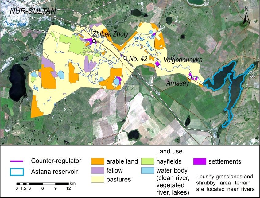
Water 2020, 12, 2672                                                                                 2 of 20

parallel computing and cloud-computing services in order to meet the high computational demand [1,6].
In addition, Geographical Information Systems (GIS) coupled with Remote Sensing (RS) data have
significantly facilitated the generation of flood hazard mapping. Remote sensing not only provides
input data for model construction, but also provides data for model validation [8]. The combination
of climate, hydrological and hydrodynamic models has extended the primary purpose from simple
inundation-area identification towards the formulation of climate adaptation and risk-mitigation
strategies [1]. However, the complex nature of flooding events as well as the uncertainties related to
modelling result in significant challenges for accurate and rapid flood modelling at high resolutions [1].
      In general, the concept of flood risk management describes a system, where flood forecasting
and flood warning systems play a key role. Flood hazard assessment, through inundation mapping
and identification of flood risk zones, is the core element for formulating any flood management
strategy [2,4,6]. Flood inundation modelling serves an important role of obtaining spatial distribution
information on inundation patterns (such as water depth and flow velocity) [9]. This could inform
inform on the severity of the hazard, any threats to public safety and potential financial losses [9].
Further, they could be used to support emergency management actions and mitigation policies for
future flooding events [10,11]. They are also critical for informing the public and policy makers and to
receiving support for the formation of suitable governance [11].
      The primary tools for performing inundation mapping are hydraulic/hydrodynamic models.
They are mostly used for the simulation of flood events, estimation of vulnerable areas, flood management
planning and the determination of spatially distributed variables of interest [2]. In general, they describe
the fluid motion and the dynamics of the flood wave by solving mathematical equations, which are based
on the principles of the conservation of mass and momentum [12]. Depending on the study area as
well as the purpose of the project, the user can choose between models with different dimensionalities
(1D, 2D, etc.), numerical schemes (finite volume, finite difference, etc.), mesh representations
(structured, unstructured, etc.) and equations (Kinematic Wave, Diffusion Wave, Muskingum, etc.).
Mihu-Pintilie et al., Patel et al. and Shustikova et al. [2,4,6] have stated that 1D modeling represents
the channel processes accurately, but for the assessment of flood wave dynamics in the floodplain,
when the capacity of the channel has been exceeded and the flow is spread across a large area in the
downstream terrain, 2D would be a better choice. Morsy et al. [13] recommend using fully 2D models
with a high degree of detail on the terrain for the purpose of avoiding the uncertainties and limitations,
which can arise from the incorrect interpretation of flood dynamics and the inaccurate representation of
the relief. According to Teng et al. and Dasallas et al. [1,5], 2D models are mostly used for flood extent
mapping and flood risk estimation, as they provide more detailed and reliable results in complex flow
simulations. 2D models that solve full shallow water equations are reported to have the capacity to
simulate the timing and duration of inundation with high accuracy, though they are data-intensive
and have a high computational demand [5,14]. These disadvantages restrict their use for real-time
flood forecasting [5]. In the same study, it was reported that they are not viable for areas larger than
1000 km2 , if a resolution of less than 10 m and/or multiple model runs are required.
      This study utilized the 2D capacity of HEC-RAS, which has, according to the literature review,
a wide range of applications and deploys different schematization complexities [6]. For example,
by coupling HEC-HMS and HEC-RAS Thakur et al. [11] generated a system, which can generate
flood inundation maps for a given precipitation event. Loi et al. [15] were able to couple SWAT and
HEC-RAS for real-time flood forecasting for the Vu Gia-Thu Bon river basin. The model results were
adequate, the magnitude and timing of peak flows were accurately predicted for individual storm
events. Mihu-Pintilie et al. [2] applied HEC-RAS 2D modelling with LiDAR data to an urban location
in order to generate improved flood hazard maps. According to the authors, their results demonstrated
sufficiently accurate information regarding vulnerability to flood hazard. Quiroga et al. [16] evaluated
HEC-RAS 2D for the generation of flood depth, duration and velocity maps in the case of the
Mamore river flood. In the study performed by Vozinaki et al. [17], it was found that 1 m DEM
shows better results than the 5 m DEM, when 1D HEC-RAS and combined 1D/2D HEC-RAS is used.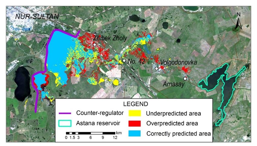
Water 2020, 12, 2672                                                                             3 of 20

Using coupled 1D/2D HEC-RAS, Patel et al. [4] simulated the flooding event caused by high release
from the Ukai Dam and obtained acceptable results. Shustikova et al. [6] performed 2D modelling of a
floodplain inundation event in Italy with HEC-RAS and LISFLOOD-FP using the same topographical
input data and found that the latter performed slightly better than the former. Another important
point was that the computation time required by LISFLOOD-FP is significantly smaller than that of
HEC-RAS for the same grid and time step chosen. The findings suggested that the specific relief
of the study area can result in ambiguities for large scale modelling, at the same time providing
plausible results in terms of the overall model performance. Salt [18] compared the applicability of
HEC-RAS (2D) and DSS-WISE for Rancho Cielito Dam Breach modelling. The results indicated that
both models provided similar results and the differing numerical schemes of each model did not
have a significant influence on the generated inundation boundaries. However, a significantly faster
simulation of DSS-WISE was opposed to the capacity of HEC-RAS for terrain modification, which might
be necessary at certain areas for which terrain data did not capture important features. Brunner [19]
evaluated the 2D capacity of HEC-RAS using the benchmark tests developed by the UK’s Joint Defra
Environment Agency. The results demonstrated that HEC-RAS performs extremely well compared
to other models (TUFLOW, MIKE FLOOD, SOBEK, etc.) that have been tested. Both equations
of HEC-RAS (Full Momentum and Diffusion Wave) showed similar results for certain scenarios to
which they were applied. Dasallas et al. [5] performed a coupled 1D-2D simulation of the Baeksan
Flooding event using HEC-RAS. The results obtained on flood inundation were similar to those
obtained by other flood models (Gerris, FLUMEN) and observed data. The authors also claim that
HEC-RAS simulated the flooded area more realistically in terms of the ideal behavior of flood dynamics.
Rangari et al. [20] assessed the possibility of HEC-RAS use for urban flood simulation for a part of
Hyderabad. Using the simulation results, risk maps were developed for different rainfall scenarios.
Whereas Kumar et al. [21] applied HEC-RAS and Global Flood Monitoring System for flood extent
mapping. The authors have reported that the results obtained and observations were in close agreement.
Costabile et al. [22] analyzed the capacity of HEC-RAS for performing rainfall-runoff simulations
at the basin scale for the tributary of the River Po. In comparison to the Diffusion Wave equation,
the Full Momentum equation has shown very similar results with respect to the 2-D fully dynamic
model (SWE-FVM) developed by the authors. HEC-RAS has demonstrated mostly overestimation
of SWE-FVM derived flooded areas, the variations in flood areas were observed to increase as the
mesh size increases and the return period decreases. In the study by Pilotti et al. [23], hypothetical
dam break analysis using Telemac 2D and HEC-RAS 2D was performed. The findings demonstrate
that both models reproduce well the experimental hydrograph in terms of shape, peak discharge and
flood wave arrival time. In addition, both hydraulic models resulted in a very similar flood extent.
Even though hydraulic modelling has demonstrated reliable results, proven its usefulness and is a
common practice around the world, there are no published records of its application in the Republic
of Kazakhstan for the simulation of floods. There are several potential reasons for this, such as the
absence of high-resolution terrain data, river bathymetry data and the lack of high-resolution data for
calibration as well as validation. At the same time, flooding due to snowmelt is common in several
regions of Kazakhstan (such as Akmola, Karaganda, North Kazakhstan and Kostanay). It has been
estimated that 1051 settlements in Kazakhstan are potentially subject to flooding, though there have
not been any flood risk assessment studies. In addition to the natural causes (such as rapid snowmelt
and river ice-jams) of flood events, construction of houses in the water protection zones have been
reported as a cause [24]. The government expenditure for flood prevention and elimination of flood
events’ consequences for the years 2015, 2016 and 2017 constituted 134.4, 61.97 and 34.6 million USD,
respectively. In the Akmola region alone, where our study area is located, the economic losses from
floods in 2015 comprised around 49 million USD. Regarding the influence of climate change on the
occurrence of flooding events in Kazakhstan, the study by CAREC [25] reported that for the River
Zhabay, for example, spring floods may become more common and intense, if not routine in the future.
Hydraulic modelling could have also been useful for dealing with the recent event in Uzbekistan.
Uzbekistan. On 1 May 2020, the Sardoba dam collapsed, resulting in the displacement of thousands
of people and serious economic losses to Kazakhstan and Uzbekistan. Conduction of probabilistic
dam break analysis studies beforehand using hydraulic modelling could have helped for the
evacuation actions as well as for the consideration of protection measures. All of these highlight the
            Water 2020, 12, 2672                                                                          4 of 20
areas which could potentially benefit from the use of hydrodynamic modelling. The current study as
a pilot project is therefore concerned with the application of the hydrodynamic model HEC-RAS for
            On 1 May 2020, the Sardoba dam collapsed, resulting in the displacement of thousands of people
the purposeand
             of serious
                  identifying     the inundation areas during flooding events of different return periods.
                            economic losses to Kazakhstan and Uzbekistan. Conduction of probabilistic dam break
               analysis studies beforehand using hydraulic modelling could have helped for the evacuation actions
2. Materialsasand
               well Methods
                    as for the consideration of protection measures. All of these highlight the areas which could
              potentially benefit from the use of hydrodynamic modelling. The current study as a pilot project is
              therefore concerned with the application of the hydrodynamic model HEC-RAS for the purpose of
2.1. Study   Area
              identifying the inundation areas during flooding events of different return periods.
     The study      site and
            2. Materials  covers
                               Methods the territory between the Astana Reservoir (in the east) and the
Counter-Regulator (in the west). The reservoir is located 50 km away from the capital city of the
            2.1. Study Area
Republic of Kazakhstan, Nur-Sultan, in the eastern direction; while the Counter-Regulator is located
                  The study site covers the territory between the Astana Reservoir (in the east) and the
within the city      limits. Both structures are in principle earth embankment dams. Figure 1
            Counter-Regulator (in the west). The reservoir is located 50 km away from the capital city of
demonstrates     the study
            the Republic         area andNur-Sultan,
                           of Kazakhstan,        the location       of these
                                                           in the eastern         twowhile
                                                                            direction;     hydraulic      structures. isThe Astana
                                                                                               the Counter-Regulator
Reservoir located
            has the       primary
                     within               function
                             the city limits.          of supplying
                                               Both structures                 Nur-Sultan
                                                                are in principle                  with dams.
                                                                                    earth embankment        drinking
                                                                                                                 Figure 1water. The
            demonstrates   the study   area and the location of these  two  hydraulic   structures.
Counter-Regulator’s main function is to hold excess water from the reservoir during the spring       The Astana Reservoir
            has the primary function of supplying Nur-Sultan with drinking water. The Counter-Regulator’s main
snowmelt in     order to prevent flooding of Nur-Sultan. The reservoir was built in 1970 and the
            function is to hold excess water from the reservoir during the spring snowmelt in order to prevent
regulator inflooding
               2011.ofThere       are The
                         Nur-Sultan.     fourreservoir
                                                settlements
                                                       was built(Zhibek
                                                                   in 1970 andZholy,        Arnasay,
                                                                                 the regulator   in 2011.Settlement
                                                                                                           There are fourNo. 42 and
Volgodonovka)      in the
            settlements     study
                         (Zhibek       area,
                                  Zholy,      withSettlement
                                           Arnasay,   a total population         of aroundin8528
                                                                 No. 42 and Volgodonovka)                 people
                                                                                                    the study area, [24].
                                                                                                                    with a Among the
            total population of around 8528 people [24]. Among the four, Zhibek-Zholy is periodically subject to
four, Zhibek-Zholy is periodically subject to spring floods. The climate of this area is described as
            spring floods. The climate of this area is described as continental, with a total annual precipitation of
continental,between
              with a200–400
                        total mm
                               annual      precipitation
                                    and a temperature   rangeof   between
                                                               of −40 ◦ C to +35200–400      mm and a 25–30%
                                                                                  ◦ C [25]. Approximately    temperature
                                                                                                                     of the  range of
−40 °C to +35  °Cprecipitation
            total  [25]. Approximately
                                falls in the cold 25–30%
                                                  season. of the total precipitation falls in the cold season.

                      Figure 1.Figure
                                Location    of the
                                      1. Location    study
                                                  of the     area,
                                                         study area, hydraulic    structures
                                                                     hydraulic structures       and settlements.
                                                                                          and settlements.

     The River Yesil (Ishim) is the main river in the study area. It originates in the Niyaz Mountains
at an elevation of 561 m and flows into the Irtysh river. It is the only transboundary river which
originates in Kazakhstan [26]. It has a watershed size of 177,000 km2, a total length of 2450 km and an
average slope of 0.21‰. The study region covers approximately 56 km long section of the river. The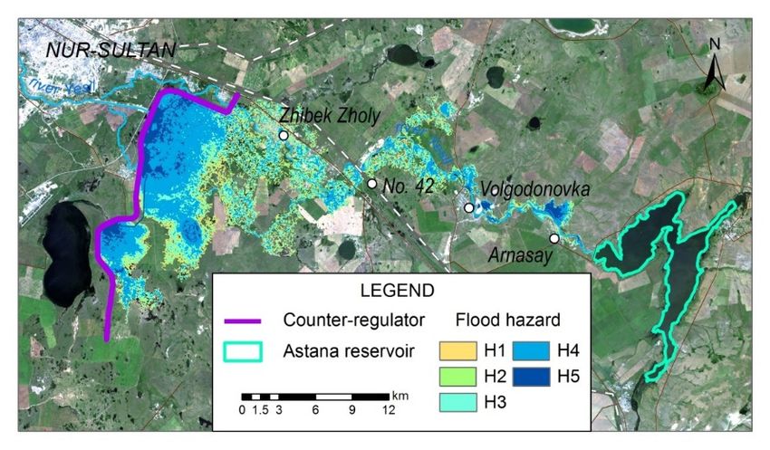
Water 2020, 12, 2672 5 of 20
The River Yesil (Ishim) is the main river in the study area. It originates in the Niyaz Mountains
at an elevation of 561 m and flows into the Irtysh river. It is the only transboundary river which
originates in Kazakhstan [26]. It has a watershed size of 177,000 km2 , a total length of 2450 km and
an average slope of 0.21%. The study region covers approximately 56 km long section of the river.
The long-term average annual flow at the Turgen station, which is located just above the Astana
Reservoir, is 4.2 m3 /s (1975–2018). The flow is characterized as heterogeneous within the hydrological
year and over years [26]. As a result, the annual volume differences between years can reach 200–300%.
The analysis of the streamflow data indicates that the flow may be divided into three characteristic
periods: (1) the highwater period from April to May (85–95% of the total annual flow); (2) summer low
water (June–October, 3–8% of the flow); and (3) winter low flow (November–March, 0–3%). Analysis of
river-flow data for the last 25 years demonstrates that the start of spring highflow has shifted to
an earlier period with an increase in overall volume, whereas the duration of the highflow period
has halved [26]. In the study conducted by CAREC [25] on the influence of climate change on the
hydrology of the upstream part of the River Yesil, the SWIM hydrological model was applied under
two climate scenarios (Representative Concentration Pathways 2.5 and 8.5). The results indicate that,
at the regional scale, the northern part of Central Asia, where our river is located, is expected to become
wetter. Under both warming scenarios (moderate and strong) for 2041–2070, the monthly peak flow of
the Yesil is expected to decrease, but it will occur over two months—March and April—as opposed to
the current peak in April.
2.2. Data Sources
Hourly water-release data as well as the hydrographs for 10, 20 and 100-year flood events were
obtained from the Republican State Enterprise Kazsushar. The data on the characteristics of the
hydraulic structures was provided by the same organization. The opening of the reservoir’s and
regulator’s gates followed the same actual operating rules. The land cover map for the whole study
area was obtained from the Akimat of Tselinograd District. Roughness coefficient for each land cover
type was assigned according to the HEC-RAS Hydraulic Reference Manual [27]. The Digital Elevation
Model (DEM) is the most important input data for 2D models. In general, 2D hydraulic models are as
good as the DEM used, because the correct topographical data influences the flood simulation results.
Even though it constitutes the basic input data and governs the accuracy of the model, such data in high
resolution is not freely available [28]. Commonly available SRTM and ASTER-GDEM datasets have a
resolution of 30 m, which for some locations may not be good enough. The importance of a correct
DEM is pointed out by Kim et al. [9], who state that the uncertainties in topographic and hydrologic
data are the main sources of uncertainty in flood predictions. It was therefore decided to improve
the accuracy of available open-source DEM by several processing steps. The original available DEM
was from Sentinel-1B, with a resolution of 10 m. It was used as a base DEM, on which improvements
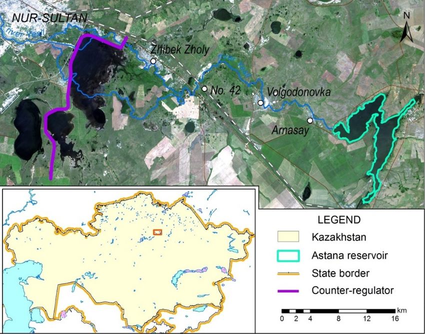
were performed. A bathymetric survey of the riverbed, which comprised an area of 305.7 hectares,
was conducted during the summer of 2019 using Sounder-Chartplotter Lowrance Elite 9 TI (Figure 2).
In addition, aerial images of the river and floodplain were taken using quadrocopter DJI Phantom
4 (with Sony EXMoR 12 .3” sensor and FOV 94o 20mm f/2.8 lense) over an area of 1696.3 hectares.
The Sentinel-1B images were processed using ESA SNAP Desktop, whereas terrain data from the aerial
images were processed in Agisoft PhotoScan Pro 4.2. As a result of processing, the resolution of the
DEM in most of the study area (90.8% of the total study area) remained at 10 m, while the areas with
bathymetric survey of the river (1.4%) and aerial photography of the floodplain (7.8%) were improved
to 2.5 m.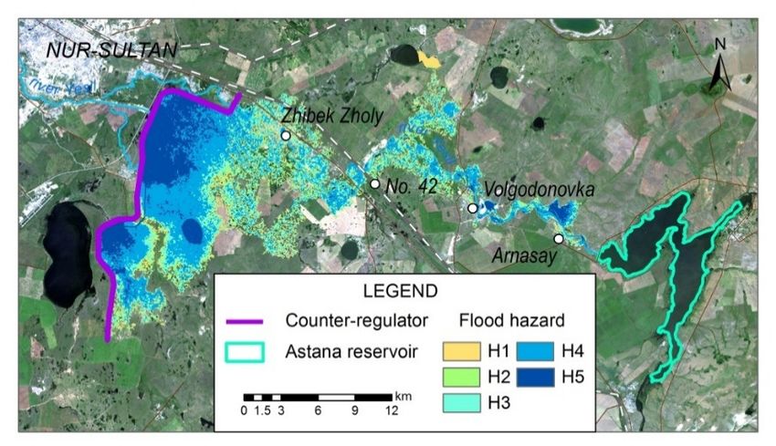
94o 20mm f/2.8 lense) over an area of 1696.3 hectares. The Sentinel-1B images were processed using
ESA SNAP Desktop, whereas terrain data from the aerial images were processed in Agisoft
PhotoScan Pro 4.2. As a result of processing, the resolution of the DEM in most of the study area
(90.8% ofWater
          the2020,
               total   study area) remained at 10 m, while the areas with bathymetric survey6 ofof20the river
                   12, 2672
(1.4%) and aerial photography of the floodplain (7.8%) were improved to 2.5 m.

                            Figure 2. Territories
                                Figure              with
                                       2. Territories withimproved   resolution
                                                           improved resolution     of DEM.
                                                                               of the the DEM.

         2.3. Hydraulic Model
               As was mentioned earlier, the Hydrologic Engineering Center’s River Analysis System (HEC-RAS
         5.0.7) was used in this project. It is a free software developed by the US Army Corps of Engineers.
         HEC-RAS is widely used for performing 1D steady and unsteady flow, 2D unsteady flow river
         hydraulics calculations, sediment transport modelling, and water quality analysis [29].
               HEC-RAS 2D uses shallow water equations, which describe the motion of water in terms
         of depth-averaged 2D velocity and water depth in response to the forces of gravity and friction.
         These equations represent the conservation of mass and momentum in a plane [1]. The finite-volume
         method used in HEC-RAS is described as advantageous, due to its conservativeness, geometric flexibility,
         and conceptual simplicity [1]. This solution approximates the average integral on a reference volume
         and allows a more general approach to unstructured mesh [4]. 2D modelling by HEC-RAS can simulate
         variability across and along the flow path. The model area is discretized into grid cells, where each
         cell uses the underlying terrain data with less loss in resolution (sub grid model). This results in the
         improvement of computational time [5]. For each cell and cell face HEC-RAS generates a detailed
         hydraulic property table (such as elevation-volume relationship, elevation-area, etc.) As a result,
         larger cells are produced, which can retain terrain details and use higher time steps. The water can
         move to any direction based on the given topography and the resistance to the flow controlled by the
         land use type and associated Manning’s coefficient [2].

         2.4. Model Generation and Assessment
              In the first step, the sub-grid modelling capacity of HEC-RAS was evaluated for the study area.
         As Kim et al. [9] state, the main purpose of mesh design is to achieve the highest degree of accuracy
         for a given computational cost. While coarser resolution allows faster simulations at the expense of
         accuracy, smaller grid sizes can represent the terrain better, but will require a longer calculation time.
         For the purpose of assessment, three different grid sizes (25, 50 and 75 m) have been used to simulate
         the same event. This would allow the analysis of grid size influence on model results. In addition,
         the available papers on HEC-RAS 2D application [2,6,16] do not consider the use of breaklines for
         mesh refinement. Thus, for the same grid size, two models were created: one with breaklines and
         another without. The breaklines included the high terrains present in the study area as well as river
         overbanks. The model performance by different grid sizes was evaluated using a high flow event from
         2017 (Figure 3). This event was chosen as this was the only year for which hourly reservoir water
         release data and remote sensing images with clear skies were available.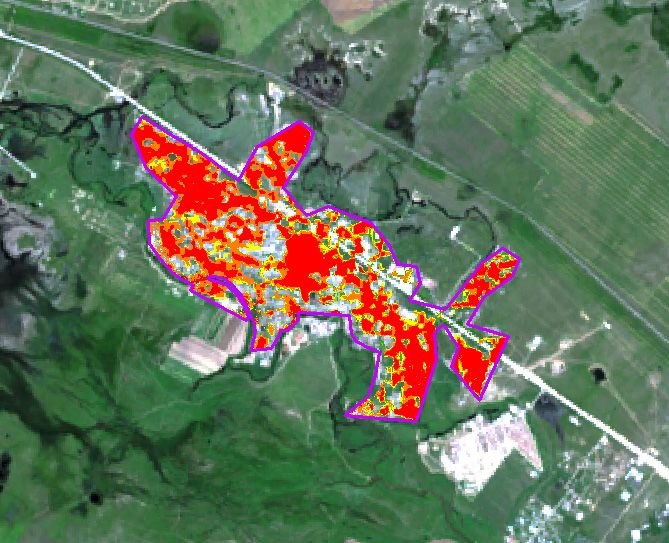
addition, the available papers on HEC-RAS 2D application [2,6,16] do not consider the use of
breaklines for mesh refinement. Thus, for the same grid size, two models were created: one with
breaklines and another without. The breaklines included the high terrains present in the study area
as well as river overbanks. The model performance by different grid sizes was evaluated using a
highWater
     flow   event
          2020,       from 2017 (Figure 3). This event was chosen as this was the only year for which
                12, 2672                                                                            7 of 20
hourly reservoir water release data and remote sensing images with clear skies were available.

                       1200

                       1000

                        800
             Q, m3/s

                        600

                        400

                        200

                          0
                              4/14/17 0:00   4/15/17 0:00   4/16/17 0:00   4/17/17 0:00   4/18/17 0:00
                                                            dd.mm.yyyy
                                                               hour

         Figure 3. Hydrograph of water release from the Astana Reservoir during spring snowmelt in April 2017.
     Figure 3. Hydrograph of water release from the Astana Reservoir during spring snowmelt in April
     2017.The total flow area comprised an area of 45,673 ha land. The release from the Astana Reservoir
   was used as an upstream boundary condition. Normal depth was used as the downstream boundary
    The total flow
   condition.       area
                In the   comprised
                        model,  wateranrelease
                                         area offrom
                                                  45,673
                                                      thehaCounter-Regulator
                                                            land. The release from  theevent
                                                                               for the  Astana  Reservoir
                                                                                             from   2017 was
wascontrolled
    used as anbyupstream   boundary
                   following         condition.
                              the same            Normal
                                         gate-opening      depth
                                                         rules   was used
                                                               adopted  by as the downstream
                                                                            Kazsushar   in 2017.boundary
                                                                                                  In order to
   have a stable model, the time step was approximated using the Courant-Friedrichs-Lewy condition.
   Simulations were performed using the Diffusion Wave equation only, due to its higher stability and
   calculation speed. Trial simulations have shown that the use of a Full Momentum equation requires
   more than 21 times longer simulation time than the simulations using Diffusion Wave equation.
   As a result, for practical purposes (for conduction of sensitivity analysis and calibration), it was not
   considered viable. Evaluation of model results was performed using the Remote Sensing Image,
   which was obtained from the website planet.com. The satellite image of the flood extent on 19th April
   2017 at 8:14:35 (UTC 00) was compared with the inundation boundary generated by HEC-RAS using
   the following Equations 1–4 from [28,30].

                                               F = (A/(A + B + C)) × 100,                                    (1)

                                                 Hit Rate (H) = A/Xobs,                                      (2)

                               False Alarm Ratio (FAR) = (Xsim/Xobs)/(A + Xsim/Xobs),                        (3)

                                       Error Bias (B) = (Xsim/Xobs)/ (Xobs/Xsim),                            (4)

   where A is the area correctly predicted as flooded (wet in both observed and simulated), B is the area
   overpredicting the extent (dry in observed, but wet in simulated) and C is the underpredicted flood
   area (wet in observed, but dry in simulated) [6,28]. Even though Equation 1 is a common method for
   comparing binary maps, it has been described as being biased in favor of overpredicting the flood
   extent [28]. The Hit Rate, also called as the probability of detection, indicates how well the model
   replicates the observed data without penalizing for overprediction [30]. The False Alarm Ratio is an
   indicator of model overprediction [30]. Error bias between 0 and 1 indicates a tendency of the model to
   underpredict and a bias between 1 and infinity indicates a tendency of the model to overpredict [30].
        After the initial assessment of different grid sizes, the selected grid size was further used to perform
   sensitivity analysis and the calibration of roughness coefficients. Afterwards, calibrated parameters
   were used for the simulation of floods of different return periods (10, 20 and 100). Flow hydrographs
   after the operation of Astana Reservoir during 10-, 20- and 100-year flood events was obtained from
   the Republican State Enterprise Kazsushar (Figure 4).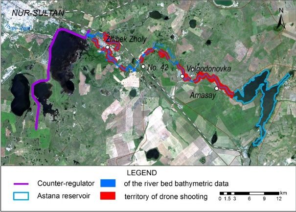
[30].
     After the initial assessment of different grid sizes, the selected grid size was further used to
perform sensitivity analysis and the calibration of roughness coefficients. Afterwards, calibrated
parameters were used for the simulation of floods of different return periods (10, 20 and 100). Flow
hydrographs after the operation of Astana Reservoir during 10-, 20- and 100-year flood events was
Water 2020, 12, 2672                                                                             8 of 20
obtained from the Republican State Enterprise Kazsushar (Figure 4).

                     1400

                     1200

                     1000

                      800
           Q, m3/s

                                                                                                     1 in 100 year
                      600
                                                                                                     1 in 20 year
                      400                                                                            1 in 10 year
                      200

                        0
                            1 2 3 4 5 6 7 8 9 10111213141516171819202428323640
                                                    day

         Figure 4. Hydrographs of water release from the Astana Reservoir during floods of 10-, 20- and 100-year
        Figure  4. Hydrographs of water release from the Astana Reservoir during floods of 10-, 20- and
         return period.
        100-year return period.
     The flood inundation areas generated were classified according to Flood Hazard classes
(Classification 1) from MLIT [2]. This classification considers five classes, which are shown in
Table 1.

                                    Table 1. Flood hazard classification according to MLIT [2].

                                    Flood Hazard         Flood Depth (m)         Hazard Classes
                                          H1                  5                   Extreme

     In addition to the classification from MLIT [2], more comprehensive flood hazard classification
system (Classification 2) was developed for Kazakhstani conditions (Table 2). This system considers
not only water depth, but also flow velocity as well as flood duration. The classification criteria were
based on the natural characteristics of the study area and the impact of past flood events.

                            Table 2. Flood Hazard classification developed for Kazakhstani conditions

                     Hazard Level       Flood Depth, m        Flow Velocity, m/s        Flood Duration, Hours
                         Low               up to 1                up to 0.01                     up to 5
                      Medium                 1–3                  0.01–0.05                        5–24
                        High                 3–5                   0.05–0.1                       24–72
                        Crisis               5–7                    0.1–1.0                       72–120
                     Catastrophic         more than 7            more than 1.0                 more than 120

3. Results

3.1. Performance of Different Grid Sizes
      The performances of different grid sizes in simulating the flood event from 2017 with and without
breaklines are shown in Table 3. An additional row shows the results of the model with the octagonal
mesh and breaklines. In comparison to the default rectangular mesh, the octagonal mesh allows water
to flow in eight directions. As can be seen, the performance of the model did not vary significantly
between different model versions with the initial Manning’s values. The maximum coefficient (58.7%)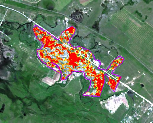
Water 2020, 12, 2672                                                                                      9 of 20

was obtained in the case of 75-m mesh without breaklines and the lowest performance (57.9%) was
observed for the 75-m and 25-m mesh with breaklines. The results indicate that the inclusion of
breaklines did not significantly affect the model performance. Interestingly, the 75-m mesh model
without breaklines showed a better performance than the same model with breaklines. There was no
improvement in the case of the 25-m mesh without breaklines.

                       Table 3. Model performance and simulation length at different grid size.

                                       Model Performance,                                   Simulation Length
           Model Version                                         H        FAR        B
                                             F (%)                                             (Minutes)
      25-meter with breaklines                 57.9             0.77    0.00011     1.22          1064
     25-meter without breaklines                58              0.77    0.00011     1.21          1271
      50-meter with breaklines                 58.4             0.79    0.00011     1.28           72
     50-meter without breaklines               58.2             0.77    0.00011     1.21           106
      75-meter with breaklines                 57.9             0.77    0.00011     1.22           28
     75-meter without breaklines               58.7             0.77    0.00011     1.17            23
      50-meter with breaklines
                                               58.1             0.77    0.00011     1.22           103
         (octagonal mesh)

      In the case of the 50-m mesh, there was indeed a slight improvement in the model’s performance.
The octagonal mesh with a 50-m grid size demonstrated similar results to the 50-m mesh without
breaklines. In terms of the Hit rate (H), all the model versions showed similar values (0.77), except for
the 50-m mesh with breaklines (0.79). There was no variation among the model versions in terms
of the False Alarm Ratio (FAR) value. Error bias (B) values demonstrate that all the model versions
overpredict the flood extent. Interestingly, the highest overprediction was observed for 50-m mesh with
breaklines, whereas the lowest overprediction was for 75-m without breaklines. Even though the mesh
size did not have a significant influence on the model’s performance, there was a significant difference
in terms of simulation length. The longest time (>17.5 h) was observed for the 25-m mesh, whereas the
shortest time was for the 75-m mesh (23–28 min). The 50-m mesh (both octagonal and rectangular)
had a simulation time of 72–106 min. It is interesting to observe that even though the inclusion of
breaklines did not significantly influence the model’s performance, it did have an influence on the
duration of the simulation. For the 25-m and 50-m meshes in particular, the inclusion of breaklines
shortened the duration of the simulation. The reason for this could be the earlier leakage of water
from the river cells to the floodplain cells in the case of the model without breaklines. This would
consequently result in calculations at each time step taking place in more cells than for the case, where
the leakage starts later due to the breaklines acting as barriers for flow. However, this was not the case
for the 75-m mesh, where the opposite trend was observed.
      Considering the model’s performance for each mesh size, further simulations were done using
the 50-m mesh model. This version was chosen for several reasons: (1) the simulation length was not
as long as the 25-m mesh; (2) its version with breaklines performed better than the 75-m mesh with
breaklines; and (3) it would consider more land-use types than 75-m mesh (depending on the study
area). The last point is related to the structure of HEC-RAS 2D, which only allows one roughness
coefficient per side. Specifically, during calculations it uses the land use type, which is located in the
middle of the cell face.

3.2. Sensitivity Analysis and Calibration
     Sensitivity analysis for land use types present in the study area was done using the 50-m mesh
with breaklines. There were 33 land use types in total, 10 of which were found to be more sensitive
than the others (Figure 5).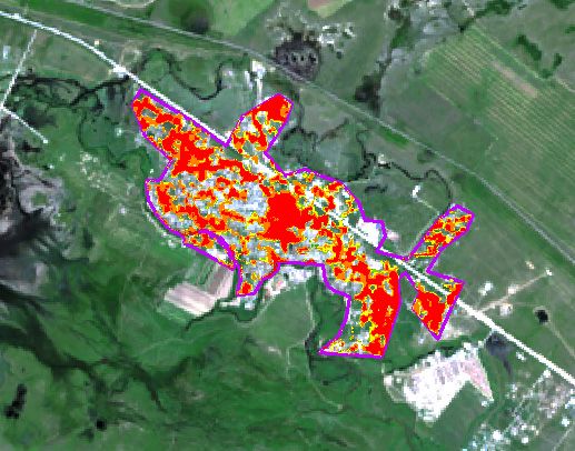
middle of the cell face.

3.2. Sensitivity Analysis and Calibration
     Sensitivity analysis for land use types present in the study area was done using the 50-m mesh
with  breaklines.
Water 2020,       There were 33 land use types in total, 10 of which were found to be more sensitive
            12, 2672                                                                          10 of 20
than the others (Figure 5).

                       Figure
                       Figure 5.
                              5. Map
                                 Map of
                                     of the
                                         the sensitive
                                             sensitive land
                                                        land use
                                                             use types
                                                                 types present
                                                                       present in
                                                                               in the
                                                                                  the study
                                                                                      study area.
                                                                                            area.

     These land
            land use
                  use types
                       typesand
                              andtheir
                                  theirparameter
                                        parameterranges
                                                   ranges
                                                        areare shown
                                                            shown       in Table
                                                                     in Table 4 in4order
                                                                                    in order of decreasing
                                                                                         of decreasing area.
area. After the  sensitivity analysis, manual calibration by  trial and  error was   performed  with
After the sensitivity analysis, manual calibration by trial and error was performed with these 10 landthese
use types using the override regions function of HEC-RAS. In each simulation, only 1 roughness
coefficient was modified and the rest were kept the same. Calibration by modifying all roughness
coefficients at once (by giving different values to each one in every simulation) was not considered
feasible due to the large number of possible combinations. The adopted method might not cover all the
possible options (parameter combinations), but this is the only feasible option in the case of HEC-RAS
with many roughness coefficients to calibrate. Calibration has increased the model performance in
terms of the F statistic from 58.4% with initial parameters to 59.7% with calibrated parameters.

                           Table 4. Calibrated land use types and their parameter ranges.

                Land Use Type           Area (ha)      Minimum         Maximum         Calibrated Value
                   Pastures               27,566          0.025            0.05              0.025
                  Arable land            7575.72           0.03            0.05              0.038
                   Hayfields              2478.8           0.02            0.04              0.055
               Bushy grasslands           1072.1          0.035            0.07              0.035
                    Fallow                830.59          0.025           0.05               0.045
                 Shrubby area             790.92          0.045            0.11              0.048
                  Settlements             781.82           0.06            0.09               0.07
                     Lakes               702.58            0.03            0.05              0.04
                  Clean river             368.9           0.025           0.045              0.03
                Vegetated river             36            0.045           0.065              0.045

     Figure 6 demonstrates the flood extent derived from the simulation using calibrated parameters.
The correctly simulated areas are shown in blue, the areas underpredicted by the model are shown in
yellow and the overpredicted areas are highlighted in red. It can be seen that there is a close agreement
between the observed and simulated inundation areas, though certain areas are overestimated. The area
upstream the Counter-Regulator is significantly overestimated. Considering the resolution of the
satellite image and other potential errors in the input data (such as DEM accuracy), the simulation
results were considered to be satisfactory.
Fallow 830.59 0.025 0.05 0.045
Shrubby area 790.92 0.045 0.11 0.048
Settlements 781.82 0.06 0.09 0.07
Lakes 702.58 0.03 0.05 0.04
Clean river 368.9 0.025 0.045 0.03
Water 2020, 12, 2672 11 of 20
Vegetated river 36 0.045 0.065 0.045
Figure 6.6.Inundation areas derived
Inundation areas from satellite
derived imagesatellite
from and simulation
imageby and
HEC-RAS (yellow—underpredicted
simulation by HEC-RAS
area, red—overpredicted area,
(yellow—underpredicted blue—correct
area, prediction).
red—overpredicted area, blue—correct prediction).
3.3. Flood Inundation Mapping
3.3. Flood Inundation Mapping
The calibrated roughness coefficients and the 50-m mesh with breaklines were used for flood
The calibrated roughness coefficients and the 50-m mesh with breaklines were used for flood
inundation modelling. The maximum flows of the 10-, 20- and 100-year return period hydrographs
inundation modelling. The maximum flows of the 10-, 20- and 100-year return period hydrographs
corresponded to 744, 962 and 1289 m33 /s, respectively (Figure 4). Figures 7–9 illustrate the inundation
corresponded to 744, 962 and 1289 m /s, respectively (Figure 4). Figures 7–9 illustrate the inundation
maps after hazard classification according to MLIT. Table 5 shows the results of classification (MLIT) in
maps2020,
Water after
12,hazard classification
x FOR PEER REVIEW according to MLIT. Table 5 shows the results of classification (MLIT)
11 of 19
terms2020,
Water of inundated area
12, x FOR PEER per hazard class for each scenario.
REVIEW 11 of 19
in terms of inundated area per hazard class for each scenario.
Figure 7. Hazard map (Classification 1) produced from the 100-year return period flow hydrograph.
Figure 7.
Figure Hazard map
7. Hazard map (Classification
(Classification 1)
1) produced
produced from the 100-year return period flow hydrograph.
Figure 8.
Figure Hazard map
8. Hazard map (Classification
(Classification 1)
1) produced
produced from
from the
the 20-year
20-year return
return period
period flow
flow hydrograph.
hydrograph.
Figure 8. Hazard map (Classification 1) produced from the 20-year return period flow hydrograph.Water 2020, 12, 2672 12 of 20
Figure 8. Hazard map (Classification 1) produced from the 20-year return period flow hydrograph.
Figure 9.
Figure Hazard map
9. Hazard map (Classification
(Classification 1)
1) produced
produced from
from the
the 10-year
10-year return
return period
period flow
flow hydrograph.
hydrograph.
Table 5. Results of flood hazard classification (Classification 1) for each scenario.
Table 5. Results of flood hazard classification (Classification 1) for each scenario.
Hazard Classification Water Depth 100 Year (ha) 20 Year (ha) 10 Year (ha)
Hazard Classification Water Depth 100 Year (ha) 20 Year (ha) 10 Year (ha)
H1 (very low) 0–0.5 m 2345.7 2192.54 2218.3
H1 (very low)
H2 (low)
0–0.5 m
0.5–1m
2345.7
2331.8
2192.54
2175.43
2218.3
2159.64
H2
H3 (low)
(medium) 0.5–1m
1–2 m 2331.8
4284.8 2175.43
3781.45 2159.64
3903.53
H3 (medium)
H4 (high) 1–22–5mm 4284.8
8327.05 3781.45
7259.43 3903.53
6372.27
H5(high)
H4 (extreme) 2–5>5mm 4469.4
8327.05 1666.72
7259.43 852.83
6372.27
Total area (ha) 21,758.75 17,075.57 15,506.57
H5 (extreme) >5 m 4469.4 1666.72 852.83
According to Table 5, the simulation of the 100-year flow hydrograph resulted in the largest area
classified as being under extreme hazard. The same can be observed for the Medium and High Hazard
classes. There was no significant difference in the size of the inundation area for very low and low
hazard classes between the three events. The total inundation area shows a distinct trend towards
decrease as the return periods of the flow hydrographs decrease. Such a classification identifies the
areas which are prone to flooding and is a useful tool during the adoption of flood mitigation measures.
Tables 5–7 show the areas of each settlement located in our study area which are classified to be under
a particular hazard class according to Classification 1. The largest inundation is observed for Zhibek
Zholy (Table 6), where the total inundated area increased from a 10 to a 100-year flood event. In all
three scenarios, the largest inundated area was observed for the medium hazard class. The 100-year
event resulted in 3.2 ha of land being affected by the flood with a depth of more than five meters; 172 ha
of land had a water depth of around 1–2 m. In the case of settlement No. 42 (not shown), there was
only very low hazard level in all three scenarios. The area under this hazard class was also small for all
three scenarios (Water 2020, 12, 2672 13 of 20
as medium hazard. As can be seen from Table 8, the village of Arnasay is the second settlement to
experience significant flooding in terms of the total area of inundation. The 100-year event resulted in
13.7 ha of land having a water depth of 2–5 m, and 14.8 ha of the total settlement area was classified as
medium hazard.
Table 7. Areas affected by the floods of different return periods for the settlement Volgodonovka
(Classification 1).
Hazard Class Water Depth 10 Year (ha) 20 Year (ha) 100 Year (ha)
H1 5 m 0.00 0.00 0.00
Total area 0.28 0.60 35.77
Table 8. Areas affected by the floods of different return periods for the settlement Arnasay
(Classification 1).
Hazard Class Water Depth 10 Year (ha) 20 Year (ha) 100 Year (ha)
H1 5 4.78
0.05 9.79
0.23 13.73
0.81
TotalH5
area >5 m 0.05
15.58 0.23
38.25 0.81
57.52
Total area 15.58 38.25 57.52
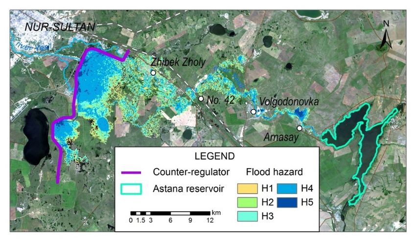
Hazard maps generated using the Classification 2 are illustrated in Figures 10–12. Whereas the
Hazard maps
corresponding generated
Table using
9 indicate thethe Classification
areas classified 2toare beillustrated in Figures
under a certain 10–12.
Hazard Whereas
class for each the
corresponding Table 9As
scenario simulated. indicate the areas classified
the Classification to be several
2 integrates under avariables
certain Hazard class
(such as for each
water depth,scenario
flow
simulated.
velocity and As flood
the Classification
duration) than2 integrates several variables
the Classification (such as water
1, it is considered depth,
to be moreflow velocity
useful. Tableand9
flood duration)
indicates than the
that when Classification
Classification 2 is 1,used
it is much
considered
larger to be more
area useful.
is under Table 9 hazard
the highest indicates that
class.
Among
when the hazard classes
Classification 2 is usedlow and larger
much medium areaclasses comprise
is under significantly
the highest hazardsmall
class.area
Amongin comparison
the hazard
to other
classes lowclasses in all scenarios.
and medium The areassignificantly
classes comprise classified to small
be under
area medium and high
in comparison classes
to other were in
classes not
all
significantly
scenarios. Thedifferent between
areas classified 3 scenarios.
to be under medium The area classified
and high classestowere
havenot
low hazard class
significantly was
different
significantly
between large for
3 scenarios. The100area
year flood event
classified to havethanlow forhazard
10 andclass
20 yearwas events. The classes
significantly large for crisis
100andyear
catastrophic
flood event thanshow foran10increasing
and 20 yeartrend in terms
events. Theof area as
classes the and
crisis return period of the
catastrophic showflooding events
an increasing
increases.
trend in termsOverall,
of areathis
as classification resulted
the return period of theinflooding
a significantly
events different
increases.flood hazard
Overall, thispattern than
classification
the Classification
resulted 1.
in a significantly different flood hazard pattern than the Classification 1.
Figure10.10.Hazard
Figure mapmap
Hazard (Classification 2) produced
(Classification from the
2) produced 100-year
from the return period
100-year flowperiod
return hydrograph.
flow
hydrograph.Figure 10. Hazard map (Classification 2) produced from the 100-year return period flow
Water 2020, 12, 2672 14 of 20
hydrograph.
Water 2020, 12, x FOR PEER REVIEW 14 of 19
Figure
Figure 11. 11. Hazard
Hazard mapmap (Classification
(Classification 2) produced
2) produced from
from thethe 20-year
20-year return
return period
period flow
flow hydrograph.
hydrograph.
Figure
Figure 12.12. Hazard
Hazard mapmap (Classification
(Classification 2) produced
2) produced from
from thethe 10-year
10-year return
return period
period flow
flow hydrograph.
hydrograph.
Table 9. Results of flood hazard classification (Classification 2) for each scenario.
Table 9. Results of flood hazard classification (Classification 2) for each scenario.
Flood Hazard Classification, Hectares
Hazard Level Flood Hazard Classification, Hectares
Hazard Level 100-Year 20-Year 10 Year
100-Year 20-Year 10 Year
Low Low 751.83
751.83 17.54
17.54 19.16
19.16
Medium 157.21 156.02 163.44
Medium High 157.21
1316.05
156.02
1520.49
163.44
1520.5
High Crisis 1316.05
4886.73 1520.49
4756.58 1520.5
4405.25
Crisis
Catastrophic 4886.73
14,646.93 4756.58
10,624.94 4405.25
9398.22
Total area
Catastrophic 21,758.75
14,646.93 17,075.57
10,624.94 15,506.57
9398.22
Total area 21,758.75 17,075.57 15,506.57
In the Figures 13 and 14 the different Flood Hazard classes present in the settlements Arnasay
In Zhibek
and the Figures
Zholy13are
andillustrated.
14 the different
TablesFlood
10 and Hazard classes
11 show present
the areas in in thesettlement,
each settlementswhich
Arnasay have
and Zhibek Zholy are illustrated. Tables 10 and 11 show the areas in each settlement,
different hazard levels. These settlements are located at different geomorphological positions and which have
different hazardconditions.
hydrological levels. These settlements
Village Arnasay areis located
located at
ondifferent
the rightgeomorphological
bank of the River positions
Yesil withinandthe
hydrological
high terraceconditions.
above the Village Arnasay
floodplain. In allisthree
located on thethe
scenarios, right bank of area,
floodplain the River
where Yesil
dry within
channelstheare
high
present, experience the greatest inundation. The largest inundation area is observed for crisisare
terrace above the floodplain. In all three scenarios, the floodplain area, where dry channels and
present, experience
catastrophic the
classes in greatest inundation.
all scenarios. 100 yearThe andlargest
20 yearinundation
events had area
similaris observed for crisis
area classified to be and
under
catastrophic classes in all scenarios. 100 year and 20 year events had similar area classified to be
under high risk, whereas 10 year event had 3 times smaller area under this class. The low hazard
class comprise significantly large area during 100 year event than during other 2 scenarios.(Classification
In the Figures2).13 and 14 the different Flood Hazard classes present in the settlements Arnasay
and Zhibek Zholy are illustrated. Tables 10 and 11 show the areas in each settlement, which have
Areas at Risk of Flooding of Various Levels, Hectares
different hazard RISK LEVEL
levels. These settlements are located at different geomorphological positions and
100-Year 20-Year 10 Year
hydrological conditions. Village Arnasay is located on the right bank of the River Yesil within the
Low 14.07 0.24 0.05
Water
high2020, 12, 2672
terrace above the floodplain. In all three scenarios, the floodplain area, where dry channels15are
of 20
Medium 2.38 1.76 0.34
present, experience the greatest inundation. The largest inundation area is observed for crisis and
High 4.75 4.78 1.43
catastrophic classes in all scenarios. 100 year and 20 year events had similar area classified to be
high risk, whereasCrisis
10 year event had 18.13 6.67under this class.
3 times smaller area 2.5 The low hazard class
under high risk, whereas 10 year event had 3 times smaller area under this class. The low hazard
Catastrophic
comprise significantly 20.16
large area during 11.7during other 27.31
100 year event than scenarios.
class comprise significantly large area during 100 year event than during other 2 scenarios.
Total area 59.49 25.15 11.63
The village Zhibek Zholy is located within a low terrace between the reaches of the Yesil River
after its bifurcation. As a result, there is higher risk of flooding in comparison to other settlements.
During the 10 year return period flood event about 30–35% of the territory of the settlement is
already subject to flooding (Figure 14). As in the case of Arnasay village, the largest inundation area
was for crisis and catastrophic hazard classes. There was no significant difference in inundation
extent for high hazard class. If 10 and 20 year events resulted in larger area under medium hazard
class than the 100 year flood event, in terms of medium hazard class an opposite trend was observed.
10 and 20 year events resulted in similar flood inundation areas for all the classes, except
catastrophic class. The obtained inundation maps and trends in inundation areas for each
Figure13.
settlement
Figure 13.Flood
Flood
could hazard
further
hazard maps
bemaps generated
usedgenerated for
for the
for developing the territory
a number
territory of
ofthe
of village
the villageArnasay
protection for
fordifferent
measures
Arnasay fromflood
different extreme
flood
events.
events. Left-100 year event, middle- 20 year flood event, right- 10 year flood event.
events. Left-100 year event, middle- 20 year flood event, right- 10 year flood event.
Figure14.
Figure 14. Flood
Flood hazard
hazard maps
maps generated
generated for
for the
theterritory
territoryofofthe
thevillage
villageZhibek
ZhibekZholy
Zholyforfordifferent
different
Figure100.
Figure 100.year
year event,
event, middle-
middle- 20
20 year
year flood
flood event,
event,right-
right-10
10year
yearflood
floodevent.
event.
Table
Table10. Areas affected
11. Areas affectedbybythe
the floods
floods of different
of different return
return periods
periods forsettlement
for the the settlement
ZhibekArnasay
Zholy
(Classification
(Classification 2).
2).
AreasAreas
at Risk of Flooding
at Risk of Various
of Flooding Levels,
of Various Levels,Hectares
Hectares
Risk
RISKLevel
LEVEL
100-Year
100-Year 20-Year
20-Year 10 Year
10 Year
Low 14.72 2.53 2
Low 14.07 0.24 0.05
Medium
Medium 6.08
2.38 15.34
1.76 13.250.34
High
High 56.82
4.75 65.124.78 66.671.43
Crisis
Crisis 159.32
18.13 138.58
6.67 141.512.5
Catastrophic
Catastrophic 20.16
298.91 11.7
211.62 186.917.31
Total area
Total area 59.49
535.85 25.15
433.19 410.3411.63
Table 11. Areas affected by the floods of different return periods for the settlement Zhibek Zholy
4. Discussion
(Classification 2).
Flooding events can cause significant economic loss and even human death. According to
Dasallas et al. [5], they are considered to have
Areas theofhighest
at Risk risk
Flooding ofamong
Varioushydro-meteorological
Levels, Hectares hazards.
Risk Level
It is therefore highly important to address these events in a20-Year
100-Year way that reduces their negative influence
10 Year
on people and infrastructure. Flood simulation using hydraulic models is one of the main tools
Low 14.72 2.53 2
Medium 6.08 15.34 13.25
High 56.82 65.12 66.67
Crisis 159.32 138.58 141.51
Catastrophic 298.91 211.62 186.91
Total area 535.85 433.19 410.34Water 2020, 12, 2672 16 of 20
The village Zhibek Zholy is located within a low terrace between the reaches of the Yesil River
after its bifurcation. As a result, there is higher risk of flooding in comparison to other settlements.
During the 10 year return period flood event about 30–35% of the territory of the settlement is already
subject to flooding (Figure 14). As in the case of Arnasay village, the largest inundation area was for
crisis and catastrophic hazard classes. There was no significant difference in inundation extent for
high hazard class. If 10 and 20 year events resulted in larger area under medium hazard class than
the 100 year flood event, in terms of medium hazard class an opposite trend was observed. 10 and
20 year events resulted in similar flood inundation areas for all the classes, except catastrophic class.
The obtained inundation maps and trends in inundation areas for each settlement could further be
used for developing a number of protection measures from extreme events.
4. Discussion
Flooding events can cause significant economic loss and even human death. According to
Dasallas et al. [5], they are considered to have the highest risk among hydro-meteorological hazards.
It is therefore highly important to address these events in a way that reduces their negative influence
on people and infrastructure. Flood simulation using hydraulic models is one of the main tools
applied for that purpose. The current study is the pilot project on the application of HEC-RAS 2D
for Kazakhstani conditions. The comparison of model performance by different grid sizes indicate
no significant difference between the results. However, there is a significant difference in terms
of simulation time between the different versions. Shustikova et al. [6] state that for large scale
studies, 50-m (for LISFLOOD-FP) and 100-m resolutions (for HEC-RAS, with 1-m terrain) offer a
compromise between accuracy and computational cost. According to our results, the 50-m mesh with
breaklines was chosen as the optimum one. Even though the use of breaklines did not significantly
influence the model’s performance, their inclusion during the mesh generation is highly recommended.
Barriers (indicated by breaklines) play an important role during flood propagation and our results
show that their inclusion can shorten the simulation time. Jarihani et al. [24] pointed out that the mesh
size in addition to DEM accuracy influences the calculation of the water inundation extent. As a result,
this could be problematic, when the model results are compared with satellite images of the flood
extent. Time savings due to larger mesh size is a key factor when the modeller is planning to perform
calibration and uncertainty analysis. It is therefore important to perform the comparison of different
grid sizes for any study area, in order to find the optimum mesh size. For the simulated event from
2017, hydrological processes such as infiltration and evaporation were considered to be negligible.
Due to the frozen condition of the soil layer, it was safe to assume no infiltration in our case. Estimation
of evapotranspiration from MOD16A2 and MYD16A2 demonstrated that during the simulation period
(14–19 April 2017) an average ETP was around 6.4 mm for the study area. This is a much lower value
than the simulated average water depth on 19 April (1.94 m) and so ETP loss was also assumed to
be negligible.
Manual calibration of the roughness coefficients produced a slight improvement in the model’s
performance. The increase is not as significant as one would have expected, and the following could
have been the reasons for that:
(1) DEM quality. If we consider the fact that the aerial images did not cover the whole river reach in
the study area, these areas without improved DEM might have acted as a place for leakage of
water. In such areas due to the resolution of the base DEM, there are no high terrains and the
river floodplain is not clearly represented. As a result, when the water level rises, there are no
barriers for water and with the low slope of the study area the water can travel a long distance and
might result in a larger inundation area. The influence of high-resolution terrain data on model
performance was demonstrated in the study by Shustikova et al. [6], where results increased
when 1-m terrain data was used in comparison to coarser data.You can also read