Hierarchical Bayesian Framework For Bus Dwell Time Prediction
←
→
Page content transcription
If your browser does not render page correctly, please read the page content below
1

   Hierarchical Bayesian Framework For Bus Dwell Time Prediction
                   Isaac K Isukapati1 , Conor Igoe1 , Eli Bronstein2 , Viraj Parimi1 , and Stephen F Smith1
                           1The Robotics Institute, Carnegie Mellon University, Pittsburgh, PA 15213 USA
       2 Department     of Electrical Engineering & Computer Science, University of California, Berkeley, CA 94720 USA

   In many applications, uncertainty regarding the duration of activities complicates the generation of accurate plans and schedules.
Such is the case for the problem considered in this paper - predicting the arrival times of buses at signalized intersections. Direct
vehicle-to-infrastructure communication of location, speed and heading information offers unprecedented opportunities for real-time
optimization of traffic signal timing plans, but to be useful bus arrival time prediction must reliably account for bus dwell time
at near-side bus stops. To address this problem, we propose a novel, Bayesian hierarchical approach for constructing bus dwell
time duration distributions from historical data. Unlike traditional statistical learning techniques, the proposed approach relies
on minimal data, is inherently adaptive to time varying task duration distribution, and provides a rich description of confidence
for decision making, all of which are important in the bus dwell time prediction context. The effectiveness of this approach is
demonstrated using historical data provided by a local transit authority on bus dwell times at urban bus stops. Our results show
that the dwell time distributions generated by our approach yield significantly more accurate predictions than those generated by
both standard regression techniques and a more data intensive deep learning approach.

   Index Terms—Task Duration prediction, Hierarchical Bayesian Models, Intelligent Transit Systems, Adaptive Control.

                          I. I NTRODUCTION                                      that significantly more accurate dwell time distributions can
                                                                                be derived from far less data than is possible with either
M       ANY practical planning and scheduling problems are
        complicated by the durational uncertainty inherent in
the tasks that must be performed to achieve stated objectives.
                                                                                standard linear regression methods, or more contemporary
                                                                                deep learning techniques.
                                                                                   The remainder of the paper is organized as follows. We
An attempt by a robot to pick up an unstable object can
                                                                                first motivate and provide background information on the
have multiple outcomes for example, and hence may require
                                                                                bus dwell time prediction problem. Next, we describe our
multiple attempts before the larger plan in which the task is
                                                                                Bayesian hierarchical modeling methodology for constructing
embedded can move forward. Alternatively, a vehicle traveling
                                                                                bus dwell time models. This is followed by a presentation
from a given pickup location to a given drop-off location
                                                                                of our empirical analysis of its effectiveness in comparison
may have several different routes to choose from, with each
                                                                                to other candidate approaches. We then briefly discuss the
route having variable duration and being dependent on current
                                                                                potential broader applicability of the work to the general
traffic conditions. Effective planning and scheduling in such
                                                                                problem of generating task models for planning and scheduling
circumstances requires the ability to accurately characterize
                                                                                systems. Finally, we summarize the main contributions of the
this uncertainty.
                                                                                paper and briefly indicate our future research directions.
   In this paper, we consider this task duration modeling
challenge in a particular setting, that of predicting bus dwell                        II. B US DWELL T IME P REDICTION P ROBLEM
times at bus stops in urban road networks. Reliable prediction
                                                                                   As indicated above, our interest in the accurate prediction of
of bus dwell times at near-side bus stops is crucial for
                                                                                bus dwell times is motivated by the opportunity that it would
determining bus arrival times at signalized intersections, which
                                                                                provide to improve the real-time dynamic flow of vehicle
in turn opens new opportunities for real-time optimization
                                                                                traffic through a network of signalized intersections. It is well
of urban traffic flows. We focus on developing probabilistic
                                                                                known that vehicle flows at signalized intersections constitute
dwell time duration models for individual bus stops from
                                                                                a non-stationary stochastic process, and optimal control of
historical data, which can then be sampled for purposes of
                                                                                those flows is NP-hard [1]. Historically, this problem has
real-time prediction. We propose a novel Bayesian hierarchical
                                                                                been approached by estimating average flow conditions and
approach to constructing probability models that offers several
                                                                                developing a fixed signal timing plan (i.e., a fixed ordering
advantages over traditional statistical learning techniques in
                                                                                and allocation of green time to various approaches at each
this application context, including the ability to start making
                                                                                intersection) offline that optimizes for these average condi-
accurate predictions with only minimal past data, the ability to
                                                                                tions. However, advances in distributed computing over the
provide robustness in the midst of a stochastic and noisy under-
                                                                                past two decades have enabled the development of online
lying system, and the ability to deliver measurable confidence
                                                                                planning approaches that produce signal timing plans in real-
in predictions. To demonstrate the efficacy of the approach, we
                                                                                time that match the actual traffic on the road. [2, 3]
present the results of experiments performed using historical
                                                                                   The Surtrac planning algorithm [3] provides a representative
data provided by a local transit authority. Our results show
                                                                                example of this online planning approach to traffic signal con-
Manuscript received June 14, 2018. Corresponding author: I. Isukapati (email:   trol. At the beginning of each planning cycle, each intersection
isaack@cs.cmu.edu).                                                             independently senses the traffic approaching in all directions
2

and constructs a prediction of when all sensed vehicles will        determination of bus schedules, has relied on linear regression
reach the intersection. This prediction is then interpreted as      prediction methods [10–13]. Furthermore, methodologies like
a special type of single machine scheduling problem, and            KNNs [14, 15], random forests [16], and deep learning [17–
solved is to produce a signal timing plan that minimizes the        23] are widely applied in time series forecasting Accordingly,
cumulative wait time of all vehicles. As each intersection          our experimental analysis in Section V uses well trained linear
begins executing its plan, it also communicates an expectation      regression, online weighted least squares, and a deep learning
to its downstream neighbors of what traffic it expects to be        based LSTM approach for performance benchmark.
sending their way, giving those intersections the “visibility”
to plan over a longer horizon. Intersection plans are executed             III. BAYESIAN H IERARCHICAL F RAMEWORK
in a rolling horizon fashion and the planning cycle at each            State-of-the-art adaptive planning systems for real-time traf-
intersection repeats every second.                                  fic control employ optimization models to decide how to
   To manage complexity, the arrival time prediction utilized       allocate scare resources among tasks for optimal performance.
by each intersection aggregates individual sensed vehicles          These systems typically assume that current unfinished tasks
that are approaching from various directions into sequences         have deterministic completion times rather than explicitly
of clusters (i.e., queues and platoons) based on proximity.         taking task duration uncertainty into account. Then, to account
Since contemporary vehicle detection devices are not typically      for dynamic behavior, optimization models are re-run upon
capable of providing mode information in real-time, clusters        the discovery of new information to generate updated optimal
in this aggregate representation treat all constituent vehicles     plans. These approaches tend to be reactive rather than proac-
similarly. Arrival time prediction of clusters is based on a        tive however, and are not likely to be effective for real-time
single ”free flow” speed parameter.                                 traffic control. To generate signal timing plans that effectively
   With the advent of technologies that support direct vehicle-     optimize overall traffic flow in the presence of buses, it is
to-infrastructure (V2I) communication, it becomes straight-         necessary to utilize more informed models of bus dwell time
forward to detect vehicle mode in real-time, and distinguish        duration that proactively quantify the uncertainty.
between different classes of vehicles (e.g., passenger vehicles,       Given this goal, our approach is to utilize the availability
buses, bicyclists, etc.) that can have very different flow pat-     of real-time (or near real-time) covariate task duration data
terns, and resulting arrival times. For example, unlike passen-     (e.g. variables that influence bus dwell times such as the
ger cars, transit vehicles make frequent stops to pick up or        number of onboarding and alighting passengers) to produce
drop off passengers with uncertain dwell times. The presence        more accurate duration models for bus dwell times at specific
of transit vehicles stopping on urban streets can also restrict     bus stops. In this context, there are several challenges. First,
or block other traffic on the road depending on stop locations.     the environment can be highly stochastic and change over
Historically, Transit Signal Priority (TSP) systems have been       time, making prediction difficult due to the large variance
introduced to streamline and expedite bus movements [4–8].          and dynamic nature of the system. Second, there is often
However, as pointed out by Isukapati et al. [9], by giving          noise and outliers in available data, necessitating a robust
unconditional priority to transit vehicles, these traffic control   approach that is not prone to overfitting. Third, the available
strategies fail to optimize the overall traffic flow.               training datasets may be small, making models with many
   With V2I communication, it will be possible to produce           parameters impractical. Fourth, a confidence in the prediction
a more accurate prediction of when buses will arrive at the         might be necessary, particularly for control decisions that must
intersection. For example, we would expect knowledge of an          gauge the uncertainty of the model. Fifth, the implementation
approaching bus with an intervening bus stop to trigger a dis-      of the model in a real-time decision-making system must
aggregation of its enclosing cluster, since the bus will block      be computationally efficient. Finally, being able to interpret
some trailing vehicles while it is stopped and hence should be      the model and understand the structure of interactions of the
the head of its cluster. A bus stop dwell time model can then       variables is always an important requirement. In the following
be used to introduce expected cluster delay and propagate the       sub-sections, we introduce a Bayesian hierarchical framework
effects to any additional blocked clusters that may reach the       that meets these requirements.
queue behind the bus before it leaves the bus stop.
   The biggest source of uncertainty in this process is reliably     A. Key Concepts Of The Framework
predicting bus dwell times. Isukapati et al. [9], summarized           Central to the framework is the concept of a rolling
the statistical characteristics of bus dwell times: 1) they vary    Bayesian update scheme. Instead of learning a model from
considerably from stop to stop, 2) in addition to seasonal          a training dataset, or using historical data from multiple
trends, the variance in dwell times over any interval is sig-       qualitatively similar time intervals, we make predictions using
nificant (so averages are not useful), and 3) given the huge        a small set of continually updated model parameter distribu-
variance in dwell time distributions, any predictive bus dwell      tions. A fundamental component of the proposed framework
time model needs to learn quickly and update distribution           involves the use of an appropriate analytical statistical model
continuously to generate useful information in the context of       that is determined offline and subsequently refined online.
real-time signal control. Consistent with these requirements,       Such a scheme has several advantages over feature-engineered
we propose a Bayesian hierarchical framework to predict bus         solutions that rely on subsets of historical data at any given
dwell times in real-time. Previous work in predicting bus dwell     time. In many real-world contexts, task duration constitutes a
times, which has focused on advance planning issues such as         highly stochastic non-stationary process. Consequently, finding
3

informative historical data for any point in time is a difficult     to fit analytic distributions. The next step is to statistically
and noise-prone endeavor, yielding little valuable signal for        analyze similarities between the empirical CDF and each of
the comparatively complex system design. In contrast, high           the analytic distributions using the Maximum Deviation Test
correlation between task duration model parameters exists            (MDT) [24].
between short intervals. As a result, there is significant value
in maintaining real-time beliefs of a predictive model and           Algorithm 1 Choose Task Duration Likelihood Function
continually updating its parameters in the light of new data.         1:   D ← chronologically ordered task duration data
This results in a lightweight framework that naturally adapts to      2:   (ti , δi ) ← time stamp & task duration of record i in D
underlying non-stationary stochastic process, quickly improves        3:   (tl , tu ) ← lower & upper bounds of time interval
with more observations, and easily generalizes to various task        4:   η ← length of time window of interest
duration prediction scenarios.                                        5:   initialize (tl , tu ) ← (0, η)
   A second key concept of the framework is its hierarchical          6:   for (ti , δi ) ∈ D do
nature – the predictions of a “lower” model can be fed in             7:         L←[]
as inputs to a “higher” model. For example, consider a task           8:         if tl ≤ ti < tu then
duration model with three input covariates [x1 , x2 , x3 ]. As        9:              append δi to L
illustrated in Fig 1, only x1 , x3 are directly observed, and x2     10:         else
is estimated by a model at different layer, and the estimated        11:              compute empirical CDF F from data in L
value of x2 in turn, feeds as an input for the main task duration    12:              fit n CDFs F 0 ← [F1 , ..., Fn ] to data in L
model. This concept is illustrated in the application section of     13:              S ← MDT scores for F & each CDF in F 0
this paper.                                                          14:              write MDT output [F, F 0 , S] to an output file
                                                                     15:              update (tl , tu ) ← (tu , tu + η)

                                                                        As the name suggests, the maximum deviation test is a
                                                                     statistical technique designed to quantify statistical differences
                                                                     between two probability density functions. The methodology
                                                                     employed here measures the statistical similarity between the
                                                                     empirical task duration distribution and each of the analytic
                                                                     distributions using MDT scores. The MDT score is defined as
                                                                     the number of percentile values in an analytic CDF (Fi0 ) that
                                                                     are within a user-defined threshold of the empirical CDF (F ).
          Fig. 1: Hierarchical Bayesian Framework                    The analytic distribution with the highest MDT score (smax ) is
                                                                     statistically most similar to the empirical distribution. Pseudo-
   The following sub-sections provide details on the individual      code for the methodology is given in Algorithm 2.
steps in using the framework.
                                                                     Algorithm 2 Maximum Deviation Test
 B. Selecting The Likelihood Function For Task Duration
                                                                      1:   tol ← error tolerance threshold
   The first step is to find an analytic distribution that best       2:   F ← empirical CDF
describes the empirical task duration distributions. Although,        3:   F 0 ← [F1 , ..., Fn ] ← CDFs of n analytic distributions
in principle, one could choose a distribution commonly used to        4:   initialize test scores S ← [0, 0, ..., 0]
model task durations, such as the log-logistic distribution, it is    5:   for Fi ∈ F 0 do
important to select the distribution that best matches historical     6:        for p in [0, 100] do
data. Unlike the training stages for many complex statistical                            F −1 (p)−Fi−1 (p)
                                                                      7:            ←        F −1 (p)     × 100
models, this analysis step, which involves fitting analytical
                                                                      8:            if abs() ≤ tol then
distributions and assessing their statistical similarities, does
                                                                      9:                si ← si + 1
not require a large amount of data.
                                                                     10:   smax ← max(S)
   Algorithm 1 describes the methodology for choosing a
                                                                     11:   return Fk corresponding to smax
task duration likelihood function. The first step is to chrono-
logically order the task duration data. The next step is to
develop empirical cumulative density functions (CDFs) F                 Most non-parametric tests, such as the Kalmagorov-
based on temporally sequential sets of observations that fall        Smirnov (KS) test [25], use maximum deviation from the
within the time window of interest. To ensure tight track-           mean as a measure to check for dissimilarity. Therefore, these
ing of time-varying parameter distributions, it is prudent to        tests fail to recognize dissimilarities in heavy-tailed, or multi-
consider intervals of time consistent with decorrelation of the      modal distributions. On the other hand, MDT uses the sum of
underlying process. In case the task durations δi in the data        deviations of every percentile of the distribution as a measure
are discretized (due to rounding errors), use Kernel Density         of dissimilarity. This property, in addition to the symmetric
Estimation (KDE) techniques to obtain a continuous CDF.              nature of the test, makes MDT a very powerful test over either
Next, use the same temporally sequential sets of observations        the KS Test or the Kullback-Leibler (KL) Divergence test [26].
4
Note that if covariate data is not available a priori for ployed.Observed data is used to perform an online Bayesian
prediction, this process can be also be used to determine an update and obtain the posterior distribution over the model
appropriate analytical distribution to estimate covariates. For parameters. These distributions are then used as priors for the
example, while selecting likelihood function for dwell time next Bayesian update, and are used to obtain the posterior
distributions, we considered the six analytical distributions due predictive distribution for the task duration. As mentioned
to their common usage in survival analysis: Non-central F, earlier, closed form solutions for the posterior distributions
Burr, Weibull, Beta, Log-normal, and Fisk (Log-logistic). We are generally not available, and often they are computed
used small samples of historical data and MDT test to identify using numerical integration [27], MCMC [28] methods, or
which of the six analytical distributions best explain the data. nested sampling techniques [29]. In this paper, we use the
Metropolis Hastings algorithm to obtain MCMC samples of
C. Setting Priors And Generating Predictions
the posterior distributions. The specific details of this algo-
rithm are presented in Algorithm 3. Posterior distributions
Algorithm 3 Real-Time Bayesian Inference for Task Duration
of the model parameters are used in computing the posterior
Under Uncertainty
task duration distribution. A choice descriptive statistic (e.g.
1: Ct ← predicted (or observed) covariates at time t mean or median) of the resulting task duration distribution
2: M ← most recent MCMC parameter samples can be used to inform control decisions. Moreover, a precision
3: σt ← lower threshold for standard deviation of M parameter (or variance) of the posterior predictive distribution
4: σr ← standard deviation to reset M provides insight into ”how good” a specific prediction is. In
5: P ← the variable to predict fact, one can make use of this information to make decisions
6: p̂t ← prediction for P generated at time t on whether to incorporate a specific prediction value in task
7: set up priors for the parameters planning and scheduling.
8: while t < ∞ do Lastly, while designing the system, it is important to pay
9: if M is not None then attention to the convergence and mixing properties of numer-
10: R ← samples of parameters from M , using Ct ical integration algorithms (in this case MCMC). Failing to
11: S ← samples of P for each parameter sample in do so may result in model parameters converging to point
R using P ’s parameterized distribution distributions. As noted by Brown et al. [30], there are three
12: Smed ← median of each sublist in S conditions under which MCMC posterior parameter estimate
13: p̂t ← mean of Smed might converge to a point distribution: 1) existence of multiple
14: if new observation for P is available then local peaks in the posterior will make it difficult for MCMC
15: pt ← new observation for P algorithm to traverse the space of parameters; 2) even if the
16: KM ← set of Kernel Density Estimates for each posterior is single mode, MCMC does not mix well due to
parameter in M the existence of equal posterior density for a large regions of
17: L ← likelihood of P , parameterized by the distri- the posterior; 3) overly informative priors favors unreasonable
butions of parameters KM and covariates Ct large branch lengths. In theory, these problems can be tackled
18: M ← samples of approximate posterior distribu- by specifying compound Dirichlet priors for branch lengths.
tion of the parameters obtained with Metropolis-Hastings However, this can also be prevented by ensuring the standard
algorithm on previous M , using L and pt deviation of the posterior does not converge to zero. In this
19: for Mi ← samples for parameter i ∈ M do work, we empirically determined lower bounds on the stan-
20: σi ← standard deviation of Mi dard deviation of each parameter distribution. If the standard
21: if σi < σt then deviation of any parameter’s posterior distribution falls below
22: µi ← mean of Mi this lower bound, the parameter is reset to have a Normal
23: Mi ← samples from N (µi , σr2 ) distribution with the same mean and a standard deviation
above the lower bound.
The next step after choosing the likelihood function(s) (the It is important to note that this algorithm is used in a rolling
output of algorithm 1) is to choose a prior distribution for each fashion to make task duration predictions for each task in real-
parameter of the task duration analytical distribution, and any time. Thus, there is no need for a training dataset to learn the
parameters necessary for other models used in the hierarchy model parameters since they are estimated online via Bayesian
for covariate estimation. If the distribution parameters are updates. As we will demonstrate in subsequent sections of this
expressed, for example, as a linear combination of input paper, this framework is able to generate highly predictive
covariates, then prior distributions for each weight must be models of task durations that are resilient to non stationary
chosen. This is a fairly straightforward process – one can stochastic processes.
either choose a predictive prior based on a historical dataset
or an uninformed prior in the absence of such data. A unique IV. E XPERIMENTAL A NALYSIS
feature about any Bayesian approach is that the impact of
A. Model Overview
the prior on the posterior predictive distribution diminishes as
more Bayesian updates are made in the light of new data. Constructing a predictive bus dwell time distribution model
Once the task duration analytic distribution and model involves three sub-tasks: 1) choosing the likelihood function
parameter priors are chosen offline, the model can be de- for posterior updates; 2) choosing principal covariates that5
influence dwell time distributions; and 3) formalizing a dwell
time model using information from the previous sub-tasks.
B. Likelihood Function For Posterior Updates
Consistent with the guidance provided in the framework
(algorithms 1 & 2), we used historical data for choosing a
likelihood function. Specifically, we used the Port Authority
of Allegheny County’s (PAAC) Advanced Vehicle Location
(AVL) weekday dataset for the period from September 2012
to August 2014 for two major bus routes – 71A and 71C.
The data is chronologically ordered, and empirical CDFs
based on every fifteen minutes of data are created. Dwell
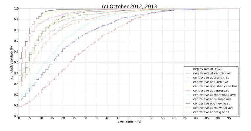
Fig. 3: Conditional dwell time distributions for several num-
times in the APCC dataset are rounded to the nearest second.
bers of onboarding passengers. Note that the variance is larger
To address this, two different continuous empirical CDFs
when more passengers board.
are generated using Gaussian, and Gamma KDE techniques.
Next, using the same temporally sequential data six analytic
distributions (Non-central F, Burr, Weibull, Beta, Log-normal, D. Dwell Time Model With Covariates
and Fisk or Log-logistic) are generated (as mentioned earlier, The following describes a Bayesian parametric model for
we choose these six analytic distributions due to their common bus dwell times using two covariates xon and xoff . Based on the
usage in survival analysis). Max-deviation scores are computed analysis presented in the subsection on choosing the likelihood
between each analytic distribution fit and each of the two function, bus dwell time is modeled as a random variable X
empirical distributions. Based on MDT scores, we chose following a Log-Logistic (Fisk) distribution. Equivalently, bus
the Log-logistic (Fisk) distribution as the likelihood for the dwell times X are distributed following the exponential of the
posterior updates. Logistic distribution. Covariate parameters are introduced by
parameterizing the s parameter, and the median of the Log-
C. Covariates For Dwell Times Logistic distribution. The exponential relationship between
In order to develop a dwell time model with covariates, the Logistic and Log-Logistic distributions is used in this
several relationships were explored between covariate data formulation. This parameterization is described below:
and dwell time, such as the number of onboarding passengers
(xon ), number of alighting passengers (xoff ), and load of the X = exp(Y ) (where Y ∼ Logistic(µ, s))
T
bus (xload ). A clear positive correlation was found between µ = ln(α) = ln(βα x + β0 )
first two covariates and dwell time, which were chosen as s = 1/τ = 1/(βτT x)
covariates in developing the predictive dwell time distribution T
model. A scatter plot demonstrating the relationship between βα = βαon βαoff
T
the number of onboarding passengers and the dwell time is βτ = βτon βτoff
presented in Fig 2. Fig 3 demonstrates not only that more T
onboarding passengers corresponds to longer dwell times, but x = xon xoff
also that the variance of the dwell time increases as more At any given time, the belief of the two parameters µ and s
passengers board. describe current belief of bus dwell time distribution. In a real-
time system with access to dwell time observations, belief of
the parameter distributions is continuously updated in the light
of new data. Bayes’ Theorem offers a natural way to achieve
such an update scheme. As only one observed dwell time d is
considered during any Bayesian update, the likelihood function
is given by
L(µ, s| ln(d)) = f (ln(d), µ, s)
Where f is the probability density function of a Logistic
distribution.
Before obtaining any posterior distributions to use as priors,
we bootstrap the model using a Normal prior for each of the 4
covariate parameters: βαon , βαoff , βτon , βτoff , and offset parameter
β0 . Once a set of posterior distributions is obtained, the most
recent posterior distributions are used as priors in the next
Bayesian update. The Metropolis Hastings algorithm is em-
ployed to obtain MCMC samples of the posterior distributions
for four covariate parameters and the offset parameter.
Fig. 2: Scatter plot of # onboardings vs. dwell times6
To make a dwell time prediction for an approaching bus, we bench-marking purposes. We trained a linear regression model
observe values for covariates xon , and xoff , and use posterior on September 2012 and tested on October 2012, which are
distributions of each β to determine the posterior predictive good training and test datasets since it is widely accepted that
distribution of X. seasonal trends in bus dwell time distributions are statistically
This process is repeated in the light of new data, using the similar [9] (also, readers interested in dwell time distribution
most recent posterior distributions of each β as priors in the models can find comprehensive reviews in [9]). Therefore,the
next Bayesian update. The means and standard deviations of linear regression model is not really put to the test. In principle,
several model parameters are shown in Fig 4 and 5, where a regression equations for September 2012 & October 2012
real-time prediction scenario is simulated on historical data in should look very similar, suggesting that predictions on the
a rolling fashion. test dataset should be reasonably good. However, the main
objective of this analysis is to evaluate the robustness of the
proposed framework. In other words, the goal is to check
whether the Bayesian model is able to predict dwell times
without any training and how good those predictions are
compared to predictions from a well-trained traditional model.
With these objectives in mind, the robustness of the
Bayesian framework was evaluated at twelve different bus
stops in the East End region along Centre Avenue corridor
in Pittsburgh, PA.
A. Cumulative Density Functions Of Dwell Times
Analyzing cumulative density functions (CDFs) of dwell
times provides useful insights into the reliability (presence
or absence of variance) of these distributions. From the
standpoint of stochastic dominance, the distributions with
curves furthest to the left have smaller variance in dwell time
distributions and hence are more reliable.
Fig. 4: Means of model parameters throughout simulation.
beta 1 corresponds to βα , beta 2 corresponds to βτ
Fig. 6: Cumulative density functions of dwell times
Fig 6 presents dwell time CDFs for test bus stops of interest.
It can be seen that dwell time distributions have the largest
variance at Negley Ave at Centre Ave (CDF in red), followed
by Centre Ave at Aiken Ave (blue), Centre Ave at Morewood
Ave (cyan), Centre Ave at Craig St NS (peach), and Centre
Fig. 5: Standard deviations of model parameters throughout Ave at Millvale (light grey). This information is useful because
simulation. Note that the MCMC samples are reset when the predicting dwell time distributions at these intersections is
standard deviation falls below a specified threshold. particularly hard due to their highly stochastic nature.
B. Model Performance
V. M ODEL T ESTING As mentioned earlier, the efficacy of the Bayesian model is
The efficacy of the proposed dwell time prediction model evaluated on data from October 2012. The results are bench-
was tested on bus dwell time data provided by the Port marked against well trained linear regression, online least
Authority of Allegheny County in Pittsburgh, Pennsylvania squares, and LSTM models trained offline on September 2012
for the period from September 2012 to August 2014. While data. The same Bayesian parametric model is applied to each
the dataset spans over two years, data from October 2012 is of the bus stops, and we set Normal priors for each of the
used to test the Bayesian model. We compared the results of 4 covariate parameters and the offset parameter β0 . Covariate
the Bayesian model to those of a linear regression model for parameters are updated on an ex post facto basis, and dwell7
TABLE I: Model Performance Comparisons
[-5, 0] [0, 5] [-5, 5]
Bus Stop
L.R Fisk O.L.S LSTM L.R Fisk O.L.S LSTM L.R Fisk O.L.S LSTM
AM 0.11 0.22 0.03 0.08 0.31 0.29 0.38 0.11 0.42 0.51 0.42 0.19
Centre Ave
PM 0.11 0.20 0.06 0.39 0.40 0.44 0.32 0.17 0.51 0.64 0.38 0.22
at Aiken Ave
All 0.10 0.21 0.02 0.08 0.39 0.41 0.37 0.13 0.49 0.63 0.39 0.21
AM 0.13 0.18 0.02 0.02 0.13 0.33 0.16 0.05 0.27 0.51 0.19 0.07
Negley Ave
PM 0.08 0.14 0.05 0.08 0.09 0.33 0.17 0.10 0.16 0.47 0.22 0.18
at Centre Ave
All 0.10 0.15 0.02 0.07 0.11 0.32 0.16 0.08 0.21 0.46 0.17 0.15
AM 0.20 0.33 0.07 0.26 0.59 0.52 0.61 0.57 0.79 0.84 0.68 0.83
Negley Ave
PM 0.13 0.21 0.07 0.60 0.66 0.66 0.78 0.32 0.79 0.87 0.85 0.92
at # 370
All 0.15 0.29 0.02 0.19 0.63 0.57 0.71 0.66 0.78 0.86 0.73 0.85
AM 0.23 0.31 0.04 0.16 0.45 0.48 0.35 0.22 0.69 0.79 0.39 0.38
Centre Ave
PM 0.18 0.26 0.20 0.07 0.55 0.47 0.60 0.37 0.73 0.73 0.80 0.44
Opp Neville St
All 0.21 0.29 0.02 0.12 0.51 0.50 0.50 0.34 0.72 0.79 0.52 0.46
AM 0.25 0.36 0.03 0.11 0.54 0.45 0.62 0.45 0.79 0.80 0.65 0.57
Centre Ave
PM 0.22 0.27 0.15 0.22 0.48 0.48 0.69 0.23 0.70 0.75 0.84 0.46
at Shadyside Hos
All 0.20 0.30 0.03 0.15 0.52 0.46 0.53 0.28 0.73 0.76 0.56 0.43
AM 0.16 0.25 0.05 0.08 0.38 0.35 0.41 0.12 0.54 0.61 0.46 0.20
Centre Ave
PM 0.15 0.37 0.11 0.12 0.58 0.44 0.44 0.35 0.73 0.81 0.55 0.47
at Morewood Ave
All 0.15 0.28 0.07 0.10 0.52 0.45 0.43 0.18 0.67 0.73 0.50 0.28
AM 0.14 0.25 0.16 0.10 0.41 0.45 0.49 0.18 0.54 0.71 0.65 0.27
Center Ave
PM 0.18 0.35 0.25 0.16 0.50 0.44 0.53 0.25 0.68 0.79 0.79 0.41
at Millvale Ave
All 0.13 0.28 0.03 0.11 0.51 0.50 0.39 0.17 0.65 0.78 0.41 0.28
AM 0.21 0.25 0.02 0.12 0.46 0.51 0.58 0.23 0.67 0.76 0.60 0.35
Centre Ave
PM 0.23 0.30 0.15 0.14 0.54 0.50 0.54 0.33 0.77 0.79 0.70 0.47
at Melwood Ave
All 0.20 0.28 0.02 0.11 0.54 0.52 0.54 0.24 0.74 0.80 0.56 0.35
AM 0.17 0.34 0.07 0.16 0.57 0.44 0.62 0.31 0.73 0.78 0.69 0.47
Centre Ave
PM 0.24 0.34 0.15 0.21 0.53 0.42 0.48 0.26 0.76 0.76 0.64 0.47
at Graham St
All 0.19 0.31 0.02 0.16 0.59 0.48 0.53 0.25 0.78 0.80 0.55 0.41
AM 0.19 0.30 0.09 0.07 0.55 0.47 0.59 0.30 0.74 0.77 0.68 0.37
Centre Ave
PM 0.09 0.26 0.15 0.24 0.53 0.42 0.65 0.24 0.62 0.68 0.80 0.47
at Cypress St
All 0.16 0.26 0.11 0.10 0.54 0.46 0.68 0.22 0.70 0.73 0.79 0.31
AM 0.07 0.17 0.03 0.11 0.25 0.32 0.30 0.16 0.32 0.49 0.33 0.28
Centre Ave
PM 0.15 0.13 0.18 0.06 0.26 0.30 0.38 0.18 0.42 0.43 0.55 0.24
at Craig St NS
All 0.11 0.17 0.02 0.08 0.26 0.34 0.33 0.15 0.37 0.51 0.34 0.23
AM 0.22 0.32 0.04 0.29 0.60 0.51 0.42 0.44 0.82 0.82 0.46 0.74
Centre Ave
PM 0.21 0.28 0.14 0.23 0.54 0.50 0.65 0.30 0.76 0.78 0.80 0.53
Opp Shadyside Hos
All 0.21 0.29 0.04 0.16 0.57 0.49 0.46 0.36 0.79 0.78 0.49 0.52
time predictions are made starting from the very first new data
point onward.
We use the ability to predict dwell times within a small error
threshold as a performance metric to evaluate the models. The
rationale for choosing small error bounds is to account for
the fact that these dwell time values are used by planning
algorithms in real-time systems, so larger errors will generate
schedules that are far from optimal. For this reason, the
fraction of predictions within error bounds of [-5, 5] seconds
is used as a performance metric. Effectively, this fraction
represents the area under the error distribution density function
within these tolerance bounds. This is a more informative
metric in the context of traffic signal scheduling due to
the importance of maximizing the proportion of very close
predictions.
Table I summarizes the performance of these four models. Fig. 7: Fraction of absolute prediction error within a threshold
As can be seen, this table contains three sets of performance for our framework vs. linear regression. Note that the Bayesian
comparisons: 1) morning peak hour (“AM”, 7:00 - 10:00 AM); hierarchical model has a higher proportion of small errors.
2) evening peak hour (“PM”, 4:00 - 7:00 PM); and 3) the
entire test dataset (“All”). This table has four columns: the
first column presents bus stop location information; the second
column presents fraction of dwell time predictions with an models. This is very encouraging to see as it validates the
error between -5 and 0 seconds; and the third and fourth main philosophy behind the development of this framework,
columns contain similar information but for ranges of [0, 5] i.e., to develop a predictive probabilistic model for estimating
and [-5, 5] seconds respectively. Lastly, each row contains task durations without making use of large training datasets.
results for a specific bus stop. Second, for the scenarios in which dwell time distributions are
The following inferences can be drawn based on these highly stochastic (see Fig. 6), the Bayesian prediction model
results: First, for the most part, the Bayesian predictive model significantly outperforms the other models (refer to results for
performs at least as good as or better than the other three Negley Ave at Centre Ave, Centre Ave at Aiken Ave, and8
Absolute Residual Distribution Fisher information, which is the negative expectation of the
NEGLEY AVE AT CENTRE AVE second derivative of the log likelihood.
1.0
log p(y|λ) = −log (y!) + ylog (λ) − λ(log likelihood)
0.8
−y
The second derivative of the above function is equal to λ2 .
0.6
Fraction
−y 1
J(λ) = −E[ |λ] =
0.4
λ2 λ
1 1
J(λ) 2 = √
0.2
λ
Online least squares The previous equation can be treated as Ga( 12 , 0). Note that
0.0
Fisk this is an improper Gamma distribution, but it is acceptable
0 10 20 30 40 50 60 for the purpose of Bayesian updates.
Residual Threshold
In order obtain a posterior arrival rate distribution via a
Bayesian update, a list of observed arrival rates are maintained,
Fig. 8: Fraction of absolute prediction error within a threshold which are defined by the number of onboardings divided by the
for our framework vs. online least squares regression. headway. Once a new observation (headway and onboardings)
is made, the arrival rate is computed and appended to the
list. A new value for α is calculated as sum of the recent β
Centre Ave at Craig St NS). Fig. 7 demonstrates this trend
arrival rate observations, where β is an integer that should
for Negley Ave at Centre Ave - the Bayesian model has a
be empirically found to maximize prediction accuracy. An
much higher proportion of very close predictions than the other
onboarding prediction for an approaching bus is made by
error distributions. This again corroborates the hypothesis of
multiplying a point estimate of the posterior arrival rate
quick adaptability of the Bayesian model. Third, in addition to
distribution (e.g., mean, median) with the headway. Here the
dwell time estimates, the variance or precision parameter of the
headway information can be obtained from published bus time
Bayesian model quantifies the uncertainty of each prediction.
tables.
C. Hierarchical Bayesian Model The hierarchical model was tested at five out of twelve
intersections, and results are summarized in Table II. The
To demonstrate the ideas of hierarchical model, a variant
results are not bench-marked against any traditional learning
of dwell time estimation model is considered. This model
model, as the main idea is to demonstrate details of the
takes two input covariates: 1) estimated value of number
hierarchical Bayesian framework.
of onboardings (x̂on ), and 2) observed value of number of
alightings (xoff ). Arrival rate of passengers at a bus stop can TABLE II: Hierarchical Fisk Model
be modeled as a doubly stochastic Poisson process, and we
Bus Stop [-5,5]
developed a Bayesian model to estimate these arrival rates. AM 0.36
Centre Ave
This model uses predicted arrival rate and known bus headway at Aiken Ave
PM 0.60
All 0.50
in estimating x̂on . The model details are presented below. AM 0.43
Negley Ave
Let Yi represent the number of passengers boarding the bus at Centre Ave
PM 0.35
All 0.42
during a bus arrival event i. The arrival rate of passengers AM 0.82
Negley Ave at
at a bus stop is modeled using λ parameter of a Poisson #370
PM 0.81
All 0.83
distribution. For the purpose of Bayesian updates, the posterior AM 0.49
Centre Ave at
for λ represented by p(λ|y) is derived as: Craig St NS
PM 0.40
All 0.47
AM 0.72
λyi e−λ Centre Ave at
p(y|λ) = Πni=1 ∝ λny e−nλ Shadyside Hos
PM
All
0.78
0.67
yi !
This is the kernel of a Gamma distribution. Therefore, if
λ ∼ Ga(α, β), then VI. B ROADER A PPLICABILITY
Although our principal research interest is effectively utiliz-
p(λ|y) ∝ p(y|λ)p(λ) ing V2I communication of real-time information from buses
p(λ|y) ∝ λnȳ e−nλ λα−1 e−βλ to improve real-time traffic control decisions, we believe that
p(λ|y) = λα+nȳ−1 e−(β+n)λ the Bayesian hierarchical framework presented in this paper
has broader applicability to other planning and scheduling
p(λ|y) ∼ Ga(α + nȳ, β + n)
under uncertainty problems. To cope with uncertainty in task
where β is the number of previous observations and α is durations and outcomes, a range of techniques for building
the sum of previous arrival rates. resilient plans and schedules have emerged over the years.
A non-informative prior such as Jeffrey’s prior is used to Some techniques have relied on knowledge of uncertainty
1
bootstrap the system. So p(λ) ∝ J(λ) 2 where J(λ) is the limits to generate plans that retain temporal flexibility [31–34].9
Others have exploited probabilistic models of task duration We envision two future directions to this research: First, we
and outcome uncertainty to generate plans or policies that are interested in integrating the bus dwell time model into an
optimize expected behavior [35–39]. Still other techniques online planning algorithm like Surtrac to investigate the system
have used probability distributions to predict durations within performance improvements. Second, we want to investigate
deterministic optimization procedures [40, 41]. In all cases the efficacy of this framework in other domains of planning
however, the effectiveness of these techniques depends on the & scheduling.
availability of good probabilistic task models. R EFERENCES
There are four primary advantages of using the Bayesian [1] C. H. Papadimitriou and J. N. Tsitsiklis, “The complexity
hierarchical framework introduced above. First, it offers robust of optimal queuing network control,” Mathematics of
predictions in highly stochastic and noisy environments, which Operations Research, vol. 24, no. 2, pp. 293–305, 1999.
often have a large variance and noise in both the independent [2] S. Sen and K. L. Head, “Controlled optimization
and dependent variables that are incorporated. Second, the of phases at an intersection,” Transportation science,
Bayesian approach effectively addresses uncertainty by deliv- vol. 31, no. 1, pp. 5–17, 1997.
ering a confidence in the prediction in the form of a posterior [3] S. F. Smith, G. J. Barlow, X.-F. Xie, and Z. B. Rubinstein,
predictive distribution. Planning and scheduling systems can “Smart urban signal networks: Initial application of the
then use this confidence to inform their decisions. Third, surtrac adaptive traffic signal control system.” in ICAPS,
the framework requires little data, both in the selection and 2013.
prediction stages. The selection stage involves choosing the [4] M. Eichler and C. F. Daganzo, “Bus lanes with inter-
likelihood for the task duration variable and prior distributions mittent priority: Strategy formulae and an evaluation,”
for the model parameters, both of which can be computed from Transportation Research Part B: Methodological, vol. 40,
a small amount of historical data. In the prediction stage, the no. 9, pp. 731–744, 2006.
model can begin making predictions and updating the posterior [5] G. Zhou and A. Gan, “Performance of transit signal pri-
distribution in a rolling fashion, removing the need for a “train- ority with queue jumper lanes,” Transportation Research
ing” dataset. Fourth, the model is computationally efficient Record: Journal of the Transportation Research Board,
because analytical conjugate posterior distributions are simply no. 1925, pp. 265–271, 2005.
described by their parameters, and non-conjugate distributions [6] G. Zhou, A. Gan, and X. Zhu, “Determination of optimal
can be sampled efficiently using Markov Chain Monte Carlo detector location for transit signal priority with queue
(MCMC) methods, or nested sampling techniques. jumper lanes,” Transportation Research Record: Journal
of the Transportation Research Board, no. 1978, pp. 123–
VII. C ONCLUSIONS A ND F UTURE W ORK 129, 2006.
[7] H. Liu, A. Skabardonis, W.-b. Zhang, and M. Li, “Op-
This paper presents a hierarchical Bayesian predictive prob- timal detector location for bus signal priority,” Trans-
abilistic model for task duration predictions in real-time sys- portation Research Record: Journal of the Transportation
tems. The framework is computationally efficient, reduces the Research Board, no. 1867, pp. 144–150, 2004.
problem of overfitting, and requires little or no training to [8] J. Ding, M. Yang, W. Wang, C. Xu, and Y. Bao, “Strategy
start producing good predictions. Furthermore, unlike tradi- for multiobjective transit signal priority with prediction
tional learning models, the proposed framework effectively of bus dwell time at stops,” Transportation Research
addresses uncertainty by delivering a confidence in the predic- Record: Journal of the Transportation Research Board,
tion through the posterior predictive distribution, rather than vol. 2488, pp. 10–19, 2015.
simply supplying a point estimate. [9] I. K. Isukapati, H. Rudová, G. J. Barlow, and S. F.
The ideas presented in the framework are tested in the Smith, “Analysis of trends in data on transit bus dwell
context of predicting dwell time distributions of a transit buses times,” Transportation Research Record: Journal of the
in urban networks. Specifically, a Bayesian parametric model Transportation Research Board, no. 2619, pp. 64–74,
for bus dwell times was created using two covariates, xon , and 2017.
xoff . The efficacy of this model is tested at twelve different bus [10] K. Zografos and H. Levinson, “Passenger service time in
stops in the East end region of Pittsburgh, PA on real-world bus a no fare bus system,” Transportation Research Record,
dwell time data. The results of the model are bench-marked vol. 1051, pp. 42–48, 1986.
against those obtained from both linear and online regression [11] R. Rajbhandari, S. I. Chien, and J. R. Daniel, “Estimation
models. The results demonstrate that the Bayesian model is of bus dwell times with automatic passenger counter
able to perform at least as good as, and in most instances information,” Transportation Research Record, vol. 1841,
far better than both traditional learning models and recently no. 1, pp. 120–127, 2003.
popular deep learning models. [12] K. J. Dueker, T. J. Kimpel, J. G. Strathman, and S. Callas,
Finally, to demonstrate the ideas of hierarchical models, a “Determinants of bus dwell time,” Journal of Public
new dwell time estimation model was considered. The input Transportation, vol. 7, no. 1, p. 2, 2004.
parameter xon was estimated, whereas the other parameter xoff [13] A. Tirachini, “Bus dwell time: the effect of different fare
was observed. Model details are presented for estimating x̂on . collection systems, bus floor level and age of passengers,”
The hierarchical model was tested at the twelve intersections Transportmetrica A: Transport Science, vol. 9, no. 1, pp.
and the results do validate the usefulness of the framework. 28–49, 2013.10
[14] F. Martı́nez, M. P. Frı́as, M. D. Pérez, and A. J. Rivera, 859, 2006.
“A methodology for applying k-nearest neighbor to time [30] J. M. Brown, S. M. Hedtke, A. R. Lemmon, and E. M.
series forecasting,” Artificial Intelligence Review, vol. 52, Lemmon, “When trees grow too long: investigating the
no. 3, 2019. causes of highly inaccurate bayesian branch-length esti-
[15] F. Martı́nez, M. P. Frı́as, M. D. Pérez-Godoy, and A. J. mates,” Systematic Biology, vol. 59, no. 2, pp. 145–161,
Rivera, “Dealing with seasonality by narrowing the train- 2009.
ing set in time series forecasting with knn,” Expert [31] R. Dechter, I. Meiri, and J. Pearl, “Temporal constraint
Systems with Applications, vol. 103, pp. 38–48, 2018. networks,” Artificial Intelligence, vol. 49, no. 1-3, pp.
[16] H. Tyralis and G. Papacharalampous, “Variable selection 61–95, May 1991.
in time series forecasting using random forests,” Algo- [32] T. Vidal and G. M., “Dealing with uncertain durations
rithms, vol. 10, no. 4, p. 114, 2017. in temporal constraint networks dedicated to planning,”
[17] S. Hochreiter and J. Schmidhuber, “Long short-term in Proceedings 12th European Conference on Artificial
memory,” Neural computation, vol. 9, no. 8, pp. 1735– Intelligence (ECAI-1996), 1996, pp. 48–54.
1780, 1997. [33] P. Morris, M. Muscettola, and T. Vidal, “Dynamic control
[18] F. A. Gers, D. Eck, and J. Schmidhuber, “Applying of plans with temporal uncertainty,” in Proceedings 17th
lstm to time series predictable through time-window international joint conference on Artificial Intelligence,
approaches,” in Neural Nets WIRN Vietri-01. Springer, Seattle, WA, August 2001, pp. 494–499.
2002, pp. 193–200. [34] N. Policella, A. Cesta, A. Oddi, and S. Smith, “Solve-
[19] R. Fu, Z. Zhang, and L. Li, “Using lstm and gru neural and-robustify: Synthesizing partial order schedules by
network methods for traffic flow prediction,” in 2016 chaining,” Journal of Scheduling, vol. 12, no. 3, 2009.
31st Youth Academic Annual Conference of Chinese [35] M. Drummond, J. Bresina, and K. Swanson, “Just in-case
Association of Automation (YAC). IEEE, 2016, pp. 324– scheduling,” in Proceedings AAAI-94, 1994.
328. [36] H. Younes and R. Simmons, “Policy generation for
[20] N. Laptev, J. Yosinski, L. E. Li, and S. Smyl, “Time- continuous-time stochastic domains with concurrency,”
series extreme event forecasting with neural networks at in Proceedings ICAPS-04, Whistler, Canada, 2004.
uber,” in International Conference on Machine Learning, [37] I. Little, D. Aberdeen, and T. S., “Prottle: A probabilistic
vol. 34, 2017, pp. 1–5. temporal planner,” in Proceedings AAAI-05, 2005.
[21] K. Bandara, C. Bergmeir, and S. Smyl, “Forecasting [38] Mausam and D. Weld, “Planning with durative actions
across time series databases using recurrent neural net- in uncertain domains,” Journal of Artificial Intelligence
works on groups of similar series: A clustering ap- Research, vol. 31, pp. 33–82, 2008.
proach,” Expert Systems with Applications, vol. 140, p. [39] J. Brooks, A. Reed, E.and Gruver, and J. Boerkoel,
112896, 2020. “Robustness in probabilistic temporal planning,” in Pro-
[22] X. Qiu, Y. Ren, P. N. Suganthan, and G. A. Amaratunga, ceedings AAAI-15, 2015, p. 3239–3246.
“Empirical mode decomposition based ensemble deep [40] S. F. Smith, A. Gallagher, T. L. Zimmerman, L. Bar-
learning for load demand time series forecasting,” Ap- bulescu, and Z. B. Rubinstein, “Distributed management
plied Soft Computing, vol. 54, pp. 246–255, 2017. of flexible times schedules,” in Proceedings 6th Inter-
[23] M. R. Oliveira and L. Torgo, “Ensembles for time series national Conference on Autonomous Agents and Multi-
forecasting,” 2014. Agent Systems (AAMAS 07), Honolulu Hawaii, May
[24] I. K. Isukapati and G. F. List, “Synthesizing route travel 2007.
time distributions considering spatial dependencies,” in [41] S. Yoon, A. Fern, R. Givan, and S. Kambhampati,
Intelligent Transportation Systems (ITSC), 2016 IEEE “Probabilistic planning via determinization in hindsight,”
19th International Conference on. IEEE, 2016, pp. in Proceedings 23rd AAAI Conference on Artificial Intel-
2143–2149. ligence, 2008.
[25] R. Wilcox, “Kolmogorov–smirnov test,” Encyclopedia of Isaac K Isukapati, PhD is a project scientist at the Robotics Institute at
biostatistics, 2005. Carnegie Mellon University. Dr. Isukapati is interested in the development of
scalable mathematical and statistical models for reasoning under uncertainty.
[26] P. J. Moreno, P. P. Ho, and N. Vasconcelos, “A kullback- His other research interests include computational game theory, distributed
leibler divergence based kernel for svm classification in & multi-agent systems, travel time reliability monitoring systems, adaptive
multimedia applications,” in Advances in neural infor- signal control.
mation processing systems, 2004, pp. 1385–1392. Conor Igoe completed his bachelors in Electronic Engineering at University
College Dublin. Mr. Igoe will start his PhD in the Machine Learning
[27] L. Tierney and J. B. Kadane, “Accurate approximations Department at Carnegie Mellon University.
for posterior moments and marginal densities,” Journal Eli Bronstein is a senior in the department of Electrical Engineering &
of the american statistical association, vol. 81, no. 393, Computer Science at University of California at Berkeley.
pp. 82–86, 1986. Viraj Parimi is a Masters student in the Robotics Institute at Carnegie Mellon
[28] S. Chib and E. Greenberg, “Understanding the University.
metropolis-hastings algorithm,” The american statisti- Stephen F. Smith, PhD is a research professor at the Robotics Institute at
Carnegie Mellon University. Dr. Smith has over 35 years of experience in
cian, vol. 49, no. 4, pp. 327–335, 1995. technology development for complex planning, scheduling, and optimization
[29] J. Skilling et al., “Nested sampling for general bayesian problems. Dr. Smith is a Fellow of the Association for the Advancement of
computation,” Bayesian analysis, vol. 1, no. 4, pp. 833– AI (AAAI).You can also read