A Real Time Localization System for Vehicles Using Terrain-Based Time Series Subsequence Matching - MDPI
←
→
Page content transcription
If your browser does not render page correctly, please read the page content below
remote sensing
Article
A Real Time Localization System for Vehicles Using
Terrain-Based Time Series Subsequence Matching
Hongjuan Zhang 1,2 , Wenzhuo Li 1, *, Chuang Qian 3         and Bijun Li 1,2
 1   State Key Laboratory of Information Engineering in Surveying, Mapping and Remote Sensing,
     Wuhan University, Wuhan 430072, China; hongjuanzhang@whu.edu.cn (H.Z.); lee@whu.edu.cn (B.L.)
 2   Engineering Research Center for Spatio-Temporal Data Smart Acquisition and Application,
     Wuhan University, Wuhan 430072, China
 3   GNSS Research Center, Wuhan University, Wuhan 430072, China; qc_gnss@whu.edu.cn
 *   Correspondence: alvinlee@whu.edu.cn

 Received: 16 July 2020; Accepted: 5 August 2020; Published: 13 August 2020

 Abstract: Global Navigation Satellite Systems (GNSSs) are commonly used for positioning vehicles
 in open areas. Yet a GNSS frequently encounters loss of lock in urban areas. This paper presents a
 new real-time localization system using measurements from vehicle odometer data and data from
 an onboard inertial measurement unit (IMU), in the case of lacking GNSS information. A Dead
 Reckoning model integrates odometer data, IMU angular and velocity data to estimate the rough
 position of the vehicle. We then use an R-Tree structured reference road map of pitch data to boost
 spatial search efficiency. An optimized time series subsequence matching method matches the
 measured pitch data and the stored pitch data in reference road map for more accurate position
 estimation. The two estimated positions are fused using an extended Kalman filter model for final
 localization. The proposed localization system was tested for computational complexity with a
 median runtime of 12 ms, and for positioning accuracy with a median position error of 0.3 m.

 Keywords: real-time vehicle localization; time series subsequence matching; integrated localization
 system; dead reckoning; IMU

1. Introduction
      Autonomous vehicles and connected vehicles have emerged in recent years. This development is
linked to the rapid development of intelligent transportation systems based on advances in computing
speed, and 5G and sensor technologies. One of the key issues in all these systems is the ability to
localize a vehicle precisely. Their effectiveness is heavily dependent on lane-level or decimeter-level
ego-localization. Furthermore, the localization of the vehicles must be highly reliable to prevent failures
of these systems during operation.
      Global Navigation Satellite Systems (GNSSs) are commonly used for positioning vehicles. Given a
sufficient number of satellites, these systems can achieve centimeter-level precision by taking advantage
of Continuously Operating Reference Stations (CORS) in an open area. The BeiDou Navigation Satellite
System (BDS) in particular, has been on the rise in recent years and shows great potential in terms of
positioning and timing [1]. Combining multiple satellite systems improves the availability of signals,
gives operators more access, and increases accuracy [2]. However, GNSS frequently encounters loss of
lock in urban areas with high buildings and trees, which is averse to GNSS geometry and visibility,
degrades positioning accuracy, and can even lead to positioning failure.
      An Inertial Navigation System (INS) is an attractive augmentation of GNSS [3] that can solve this
issue. An INS has Dead Reckoning (DR) capability and can provide position, velocity and attitude
estimation even when loss of lock occurs in GNSS. At the same time, INS error can be mitigated using

Remote Sens. 2020, 12, 2607; doi:10.3390/rs12162607                      www.mdpi.com/journal/remotesensing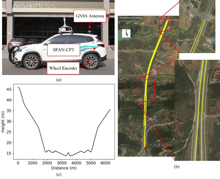
Remote Sens. 2020, 12, 2607                                                                          2 of 18

position and velocity updates from GNSS when in open areas. However, an INS suffers from drifting
errors that grow unbounded with respect to operation time, making it difficult for an INS to balance
between cost and positioning accuracy. A tactical grade inertial measurement unit (IMU) can achieve
high localization accuracy, but is too expensive to be used on a commercial scale [4]. To improve the
positioning performance of low cost inertial measurement units (IMUs), in recent years, INSs have
been combined with other sensors, like steering encoders [5], wheel tachometers [6] and odometers [7].
These sensors, however, are subject to wheel slips, road skidding and changing wheel diameters,
adding uncertainty and accumulated error to positioning results.
      Map-based localization using LiDAR [8], and cameras [9] is another common way to deal
with GNSS-denied environments. In these methods, a prior feature map is generated from point
clouds obtained from LiDAR or images, and then real-time ego-localization is performed using
feature-matching techniques. This feature-based principle is effective in environments with abundant
features such as indoors, yet, it is not suitable for outdoor environments with sparse features [10].
Moreover, LiDAR and cameras are susceptible to weather phenomena like rain, fog, and snow and
light conditions such as heavy shadow, and strong light.
      In the map-based category, terrain-based localization has also received attention, as an IMU can
measure road grades by vehicle pitch, road bank angles by vehicle rolls, or the road curvature by
vehicle yaw rate. In terrain-based localization, terrain information of the driving region is stored in a
predetermined map and new measurements of pitch, roll, or yaw angle from an in-vehicle IMU sensor are
compared with the predetermined map data to localize the vehicle. Dean et al. [11] proposed a particle
filter algorithm to obtain sub-meter longitudinal position accuracy using spatial pitch measurements
without a GNSS device. They demonstrated that the low-frequency pitch data is speed-independent so
that it is feasible to localize a vehicle by terrain disturbances in pitch. Another main contribution of
their work is the use of a particle filter, which finds the optimal position estimation from a non-Gaussian
probability distribution via similarities between the pitch measurement and pitch reference in the
predetermined pitch map, and is suitable for real-time applications. Li et al. [12] improved this method
by considering braking events of vehicles. They proposed an acceleration-considered model to take into
account the noise from braking to make the particle filter-based method more robust. Instead of using
the vehicle pitch angle, Ahmed et al. [4,13] applied this method using vehicle roll angle estimation
using low cost Micro Electromechanical System (MEMS)-IMU sensors whose external acceleration in
the lateral direction was compensated before the roll angles were calculated.
      Terrain information measured by in-vehicle sensors including pitch, roll, and yaw angles are
typical kinds of time-series sequences (TSS). TSS are defined by the explicit information about timing,
for example, electric consumption, climate data, and speech; or an ordering of values can be inferred
from the data such as handwriting [14,15]. Comparing with other kinds of time-series sequences, terrain
information also contains implicit location information. Localizing a vehicle by terrain information
becomes a pattern recognition task, specifically, a task about similarity-based pattern querying in
time-series databases.
      Problems in similarity-based pattern queries in time-series databases include the definition and
measurement of similarity in time-series sequences. The Dynamic Time Warping method (DTW) using
distance in similarity comparisons is a classic and advanced solution [16–18], which is ubiquitously
used in audio/video processing [19,20], gesture recognition [21], handwriting recognition [22],
industry [23], astronomy [24,25], medicine [26], geology [27], and finance [28]. In the last decade,
dozens of alternative measures have been suggested, like the symbolic aggregate approximation
methods [29,30], trend-based time series similarity [31], shape-based time-series similarity [14,32],
event-based time-series similarity [33], and interest point methods [34,35]. Rapid developments in
time-series matching methods make terrain-based vehicle localization more reliable and practical.
Martini et al. [36] used the Pearson-product correlation coefficient as a distance measure, instead of
DTW, to compare the road grade measurements with an off-line reference map to find a path in the
map corresponding to the location of the maximum correlation coefficient. Vemulapalli et al. [34,37]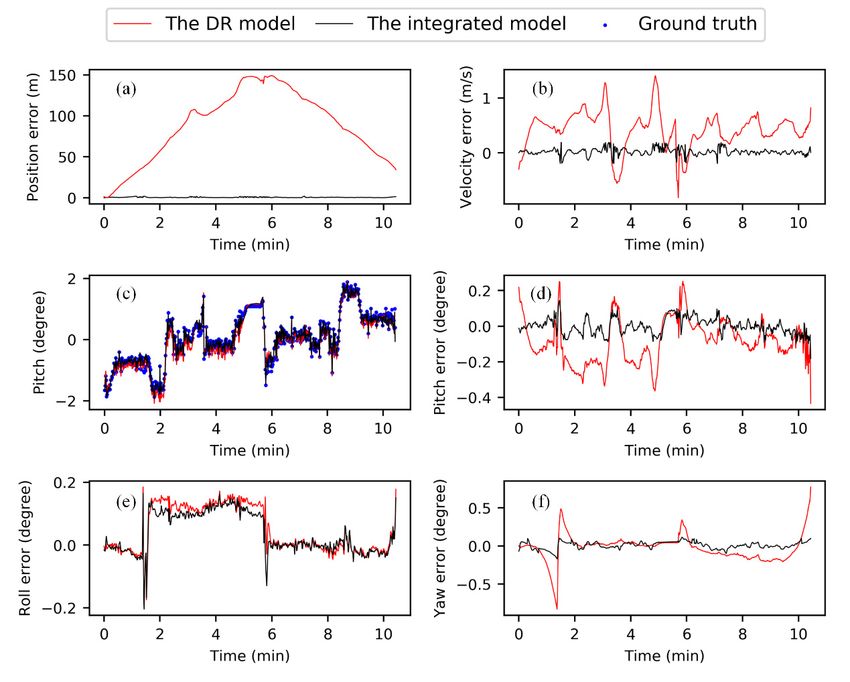
Remote Sens. 2020, 12, 2607                                                                             3 of 18

proposed a new interest point method with multi-scale extrema features, to extract feature vectors
from the pitch information of road regions and created a KD-tree in the preprocessing phase. In the
online phase, the feature vectors for a query signal were tested for a match within the feature tree to
find vehicle’s position estimation. Laftchiev et al. [38] proposed a linear model based on autoregressive
models with an exogenous input to segment the pitch data and compare model output instead of
original pitch data, which accelerates the matching process. However, in all these methods, finding
a balance between time consumption and accuracy is an elusive goal. Therefore, new approaches
must be developed to improve the viability of using advanced time-series subsequence matching
methods for vehicle localization. In this work, we present a new real-time localization system that
combines INS measurements, odometer data and an advanced DTW method to achieve both accuracy
and computation efficiency without recourse to GNSS signals.

1.1. Problem Formulation
      Previous works attempt to localize a vehicle based on terrain information using either particle
filter-based methods or solely time series subsequence (TSS) matching methods, but both have
limitations. Particle filter represents the posterior distribution of the state using a set of particles which
evolve recursively as new information becomes available [39]. Particle degeneracy is a common problem
when implementing a particle filter, which reduces the performance of the particle filter. Previous
research on particle filter-based localization [4,11–13] using terrain information addressed particle
degeneracy by increasing the particle numbers, which increased the computation burden. Moreover,
only observation information at a current moment was used to update the particles. As in [12], pitch
or pitch difference measurements have similar trends at different speeds, but at a specific location,
the values of measurements at various speeds may be at different orders of magnitude. Therefore,
using information from the current moment only is not sufficient to ensure accuracy. Consequently,
we choose to use TSS matching methods to find the path of the vehicle and current position using a
sliding window of a certain length incorporating historical data.
      DTW has been shown to be the most precise measure for time-series data queries in most
domains [16,40]. Even though previous localization research [11,34,37,38] has argued that DTW is
not computationally efficient, nevertheless authors in [16] proposed an exact DTW algorithm whose
sequential search is much faster than most alternatives. In our work, we adopted the DTW algorithm
from [16] to do TSS matching on pitch data. Furthermore, localization processes discussed in previous
research depend solely on time-series matching, regardless of accuracy, which is not robust as pitch
data varies with speed and increases the chance of matching failures.
      Another unsolved issue with pitch-based localization is that IMU error is neglected. IMU gyros
exhibit drift performances from 0.1◦ /h at a tactical grade to 100◦ /h at a typical Micro Electromechanical
System (MEMS) grade [41]. A tactical IMU alone can accomplish accurate localization but is way too
expensive to be applied broadly on consumer vehicles. A new pitch-based localization system needs
to be designed for low grade IMUs.

1.2. Contributions
    We designed a new pitch-based localization system, which has several advantages over the
methods described in the literature:

1.    An advanced DTW algorithm is used and the road map with terrain information is stored in an
      R-Tree to speed up the online localization process, which makes our system truly real-time;
2.    To ensure the accuracy at the same time, an integrated localization model is proposed to fuse
      in-vehicle multisensory data and time-series data matching results;
3.    Our proposed model is insensitive to dynamics of the vehicle velocity while most existing methods
      require steady speeds;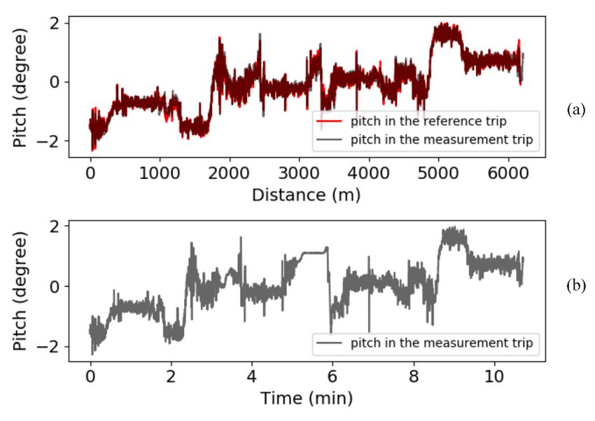
Remote Sens. 2020, 12, 2607                                                                                                4 of 18

4.    Our system is robust to abrupt changes in single-pitch data since it uses time-series subsequence
      pitch data instead of single time-point pitch data.

     The  remainder of this paper is organized as follows. The methods are described in 4Section
     Remote Sens. 2020, 12, x FOR PEER REVIEW                                                     of 19
                                                                                                        2.
Experimental implementation and the results are presented in Section 3. Section 4 provides
the conclusions.
          The remainder of this paper is organized as follows. The methods are described in Section 2.
      Experimental implementation and the results are presented in Section 3. Section 4 provides the
2. Methods
    conclusions.

     In    our integrated model, only two in-vehicle sensors are used: an odometer and a low-grade IMU,
      2. Methods
which are easily installed on almost all vehicles. The model includes an offline mapping and an online
             In our integrated model, only two in-vehicle sensors are used: an odometer and a low-grade
localization     process. In Figure 1, we illustrate our system in the online localization phase at time step k.
      IMU, which are easily installed on almost all vehicles. The model includes an offline mapping and
Measurements from IMU and odometer are combined by a Dead Reckoning (DR) model to predict
      an online localization process. In Figure 1, we illustrate our system in the online localization phase at
the navigation
      time step k. state     (latitude,from
                      Measurements         longitude,
                                                IMU andheight,
                                                          odometerroll,
                                                                     arepitch,   yaw)byofa Dead
                                                                          combined          a vehicle.    The predicted
                                                                                                   Reckoning     (DR) modelpitch
valuetois predict
            stored thein a navigation
                            vector together       with  all pitch  values   in  previous    t d seconds,    to  generate
                                          state (latitude, longitude, height, roll, pitch, yaw) of a vehicle. The          a pitch
       k . Accumulated driving distance in the t seconds is calculated by the odometer measurements,
TSS xpredicted      pitch value is stored in a vector together
                                                             d        with all pitch values in previous td seconds, to
and ifgenerate
         it is lessa pitch
                     than TSS
                            a threshold,     the predicted
                                 xk. Accumulated              navigation
                                                     driving distance       state
                                                                        in the      is returned
                                                                               td seconds         as the by
                                                                                           is calculated   result  at the current
                                                                                                               the odometer
      measurements,
time step.                 and if it is map
               From a predefined          less than
                                                whicha threshold,  the predicted
                                                        includes accurate            navigation
                                                                               positions          state is
                                                                                           and pitch        returned
                                                                                                         values        as the
                                                                                                                  of road   points,
      result   at the  current   time  step.  From   a predefined  map    which   includes  accurate
a closest road point to the vehicle can be found based on the vehicle navigation state. Given a search positions   and  pitch
      values
window,          of road
             a search       points,
                         area   in thea road
                                         closest
                                               maproad
                                                     canpoint  to thebased
                                                          be found      vehicle
                                                                              on can    be found
                                                                                   the closest      based
                                                                                                 road  point.on Then
                                                                                                                 the vehicle
                                                                                                                        a series of
      navigationk     state. Given a search window, a search area in the road map can be found based on the
pitch TSS Y from the map is generated based onk the search area. A time series subsequence matching
      closest road point. Then a series of pitch TSS Y from the map is generated based                  on the search area.
model is applied for xk and Yk to find the best-fit matching subsequence                       in Yk . An estimation model is
      A time series subsequence matching model is applied for xk and Yk to find the best-fit matching
used subsequence
      to estimate the   in Yvehicle    position model
                             k. An estimation     from the   matching
                                                         is used         model.
                                                                 to estimate    theFinally,   an integrated
                                                                                     vehicle position   from themodel   is used to
                                                                                                                   matching
integrate     the  predicted      position    from  the  DR   model   and    the  estimated     position
      model. Finally, an integrated model is used to integrate the predicted position from the DR model     from   the  matching
model,and  and
             thereturn    a final
                  estimated         vehicle
                               position      position.
                                          from           Detailed
                                                 the matching       explanations
                                                                model,   and returnofa key
                                                                                         finalmodels
                                                                                                vehicle with   greyDetailed
                                                                                                         position.   background
in Figure     1 are shown
      explanations      of keyinmodels
                                   the following
                                          with greytext.
                                                      background in Figure 1 are shown in the following text.

                      Figure 1. The
                         Figure     framework
                                1. The frameworkof
                                                 ofour
                                                    our online  localizationsystem
                                                        online localization   system  at time
                                                                                   at time      k. k.
                                                                                           stepstep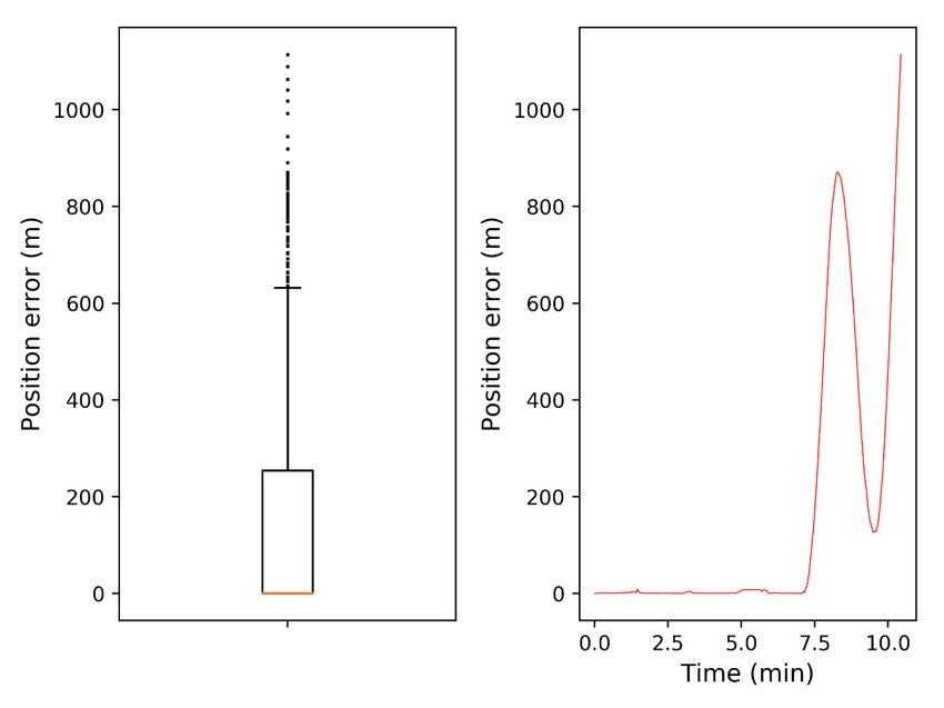
Remote Sens. 2020, 12, 2607                                                                                  5 of 18

2.1. Offline Road Map Generation
      A road map including terrain information is generated for the driving region, and all sensors are
synchronized before mapping. The vehicle must travel slowly and smoothly to gather a sufficient
number of discrete points in the test region, because the higher the resolution of the map, the higher the
                                                                              h                                   iT
positioning accuracy. The ith point of the road map is defined as pi = idi , latidi , lonidi , hidi , θidi , ∆sidi ,
where idi is the index of the point i, the values latid , lonidi , hidi , and θidi are its latitude, longitude,
height and pitch data, respectively; ∆sidi is the distance traveling from the last point, as recorded by
the odometer.
      After data acquisition, the road points are stored in an R-Tree. R-Tree is a dynamic index structure
for spatial searches [42], and can index multi-dimensional information such as geographical coordinates
in a highly efficient manner. When the point data is organized in an R-Tree, for a point, the nearest
neighbor pki within a given distance r can efficiently be queried. Even though we structure the R-Tree
by latitude and longitude information, tree nodes include all features of pi . Nodes that are in the same
bounding box are stored in a list and have consecutive index numbers. Therefore, to find a previous
neighbor whose index is idi−1 , merely requires a search for the previous node in the bounding box, or if
pi is the first node in the bounding box, a search for the last node in the previous child bounding box.

2.2. Dead Reckoning Model
     In our DR model, real-time measurements from odometer and IMU are integrated to provide a
position estimation of a vehicle. A low-cost IMU can estimate the position, attitude, and velocity of a
vehicle from the raw data: velocity increments as measured by an accelerometer and angular increments
as measured by a gyroscope, in the navigation frame. Because of the drift of the accelerometer and
gyroscope in the IMU, the velocity and angular increments from the IMU contain errors that cause the
navigation results to drift rapidly. In [43], the author elaborated estimation techniques for low-cost
inertial navigation; we however, focus on integrating an IMU and odometer, we call the DR model.
     We define the vehicle frame (v-frame) as forward-transversal-down, originating at the vehicle
center, the navigation frame (n-frame) as north-east-down, originating at the earth mass center, and body
frame (b-frame) expressed as forward-transversal-down, originating at the IMU center. More details
about the frames can be seen in [43]. The odometer is installed on the rear wheel, as it is not used for
steering. We assume that the vehicle does not have either a cross track or vertical speed but only an
along-track speed v at time step k, as measured by the odometer, so that the speed of the vehicle at the
                     h        iT
v-frame is vv,k
             wheel
                   = vk , 0, 0 . The relationship between the velocity of vehicle at the n-frame vn,k
                                                                                                  IMU
                                                                                                      and
vv,k
 wheel
       can be expressed as:

                              vn,k
                               IMU
                                   − δv n,k
                                        IMU
                                            = v n,k
                                                wheel
                                                      − δv n,k
                                                           wheel
                                                                 − C n,k
                                                                     b
                                                                           ωb,k
                                                                            nb
                                                                                ×   διb,k
                                                                                      wheel
                                                                                            ,
                                                                                                                (1)
                              with vn,k
                                    wheel
                                          = Cn,k
                                             b
                                                 Cb,k v,k
                                                  v vwheel

where δvn,k
        IMU
            and δvn,k
                  wheel
                        are the error of vn,k
                                          IMU
                                              and vn,k
                                                   wheel
                                                         , respectively. The value Cn,k
                                                                                    b
                                                                                        and Cb,k
                                                                                             v express
the rotation matrix from the b-frame to the n-frame and from the v-frame to the b-frame, while, ωb,k
                                                                                                 nb
                                                                                                     × is
the cross-product form of the rotation rate of the b-frame with respect to the n-frame, and διb,k
                                                                                              wheel
                                                                                                    is the
lever-arm vector of the odometer in the b-frame.
     Considering this relationship, the Extended Kalman Filter (EKF) is used to integrate the
measurements from the IMU and the odometer. A state vector Xk is constructed as:
                                                         T           T             T
                                       Xk = [(δϕn,k
                                                IMU
                                                    ) , (δvn,k
                                                           IMU
                                                               ) , (δpn,k
                                                                      IMU
                                                                          ) ,
                                               T         T                     T                                (2)
                                       (δεb,k      b,k                 b,k
                                          a ) , (δε g ) , δκwheel , (διwheel ) ]
                                                            k                    T

                                                        h          i
                                                   W k = wb,k  b,k
                                                          a , wg                                                (3)
Remote Sens. 2020, 12, 2607 6 of 18
•
Xk = Fk Xk +Gk Wk (4)
where superscript T is the transposition, δϕn,k
IMU
is the error in attitude as estimated by INS using the
IMU at the n-frame, δpn,k
IMU
is the error of position, δεb,k
a is the drift error of the accelerometer at the
b-frame, and the drift error of gyroscope is δεb,k
g , and δκwheel is the scale factor error of the odometer.
k
The value Wk is the noise in Xk including the white noise generated by the specific force from the
accelerator wb,k
a whose deviation is the velocity random walk of the accelerator, and the white noise of
the angular rate from the gyroscope wb,k
g whose deviation is the angular random walk of the gyroscope.
The EKF state transformation is shown in Equation (4), where Fk and Gk are coefficient matrix. Then,
Equation (4) is discretized in time so that a coarse estimation of state vector Xk− can be derived from
Xk−1 by the identity matrix I, Fk−1 , Gk−1 and Wk−1 :
Xk− = Φk|k−1 Xk−1 + Gk−1 Wk−1
, (5)
with Φk|k−1 = I + Fk−1 ∆t
The EKF observation function is constructed as follows:
Zk = Hk Xk− +Vk (6)
where Hk is coefficient matrix and Vk ∼ N 0, Rk is observation error covariance matrix.
From Equation (1) we can get:
Zk = vn,k
IMU
− vn,k
wheel
= δvn,k
IMU
− δvn,k
wheel
− Cnb ωbnb × ιbwheel
(7)
= −vn,k × δϕn,k + δvn,k − Mk δκkwheel
wheel
IMU IMU
−Cnb ωbnb × ιbwheel
so that: h i
Hk = −vn,k
wheel
× I3×3 03×9 − Mk − Cnb ωbnb × (8)
Afterwards, Xk− is updated by Zk via EKF to get Xk :
Xk = Xk− + Kk Zk − Hk Xk− (9)
T
Pk− = Φk|k−1 Pk−1 Φk|k−1 + Qk (10)
T T −1
Kk = Pk− Hk Hk Pk− Hk + Rk (11)
Pk = I − Kk Hk Pk− (12)
where Qk is the spectral density matrix, Pk the error covariance of Xk , and Kk the Kalman gain of EKF.
The estimated error Xk is fed back to the navigation state of position, velocity, and attitude in
the n-frame: n,k− n,k
pIMU δpIMU
k
p 11×3 01×3 01×3
vk 0 n,k− n,k
= 11×3 01×3 vIMU − δvIMU (13)
n,k 1×3
01×3 01×3 I + δϕn,k
n,k−
Cb IMU
× Cb 03×1
If the vk measured by the odometer drops below a certain predefined threshold, a zero-velocity
update (ZUPT) is applied instead of the wheel sensor velocity, vv,k
wheel
. More details about ZUPT
implementations can be found in [44].Remote Sens. 2020, 12, 2607 7 of 18
After estimating the current navigation state, given a predefined time duration td , we calculate
the accumulated distance dkt within td and the corresponding pitch data xk :
d
k
X h iT
dktd = ∆s j , xk = θk−td ∗ f , θk−td ∗ f +1 , . . . , θk (14)
j=k−td ∗ f
f is the sensor frequency and ∆s is the odometer increment. If dkt is less than a predefined distance
d
threshold dthre1 , then the navigation state estimated by the DR model is assumed to be the final vehicle
state. As an illustrative example, consider a vehicle stopping when a traffic light turns red, in this
condition dkt would be small and the DR model is applied for final navigation state estimation at this
d
time step.
2.3. Time Series Subsequence Matching Model
After the vehicle navigation state is calculated using the DR model and exploiting the efficiency
of an R-Tree spatial search, we calculate the closest point pki in the road map to the estimated point
pk . Given a search window [−dw , dw ], we find all road points Yk from idi−m to idi+n in the map whose
distances to pki are within this window:
h iT
Yk = pi−m , . . . , pi−1 , pki , pi+1 , . . . , pi+n ,
m
X
with argmin(| ∆sidi− j − dw |),
j=0 (15)
n
X
and argmin(| ∆sidi+ j − dw |)
j=0
Because of the drift error of an IMU, pk is the possible vehicle position, so we assume that the
accurate position drops in the set of all possible road points, Yk . We use a time series matching method
DTW to estimate the optimum position. More details about DTW are in [16]. Algorithm 1 describes
the algorithm.
Algorithm 1: Application of DTW in Localization
Initialize Variables:
Set the distance vector Dk to empty
Initialize Constant:
Cutoff frequency for a low-pass filter: fc
Algorithm Loop:
FOR l = i − m: i + n
Similar to Equation (14), from the road map find a point cluster Bk such that:
h iT
Bk = pl−u , . . . , pl−1 , pl ,
u
X
with argmin(| ∆sidl− j − dktd |)
j=0
h i
Get the pitch data vector yk = θidl−u , . . . , θidl−1 , θidl from Bk
Normalize yk and xk using Z-Score method
0
Interpolate or sample yk to yk to have the same length with xk
0
k k
Low-pass filter y and x with Fast Fourier Transform (FFT) by fc
0
Calculate the distance dl between filtered sequences yk and xk by DTW
Store dl in the distance vector Dk
END FOR
RETURN DkRemote Sens. 2020, 12, 2607 8 of 18
Normalization is necessary before executing DTW as yk and xk may be on different magnitudes.
Moreover, to reduce the noise in the measurement related to velocity, we use FFTW [45] to perform
Fast Fourier Transform (FFT) in our work. FFTW is a C subroutine library for computing the discrete
Fourier transform in one or more dimensions and is thought to be the fastest Fourier Transform tool
among all the open source FFT tools.
2.4. Estimation of Navigation State from the Matching Model
In almost all DTW applications, the best-fit matching subsequence has the smallest distance value.
In the pitch-based localization, pitch angle measurements contain bias noise and are affected by vehicle
speed. There even might be different vehicles or sensors when generating the road map and processing
online localization. Moreover, most parts of a road have slight slopes, so the magnitude of pitch angle
measurements is small. Thus, the smallest value in the Dk does not necessarily mean that we can find
the best subsequence and the right location. Instead, we choose n minima and choose the one whose
position is closest to navigation state estimation from DR, which can constraint time series matching
results. This principle makes the final navigation state more robust and precise. We use an algorithm
detecting the valleys in data to calculate Mk and mk , shown in Algorithm 2.
Algorithm 2: Calculation of Minima
Initialize Constant:
Number of minima: n
Length of xk : lx = td * f
The smallest index distance between minima: mid = ROUND(lx/n)
Algorithm Loop:
Find all valleys vk (smaller than both the left and right neighbors) in Dk and their corresponding indices ik
Sort vk by their values in ascending order and get new vk and its corresponding ik
FOR ind = 0: length of ik
Keep
h indices that is not in the range
i
ik [ind] − mid/2, ik [ind] + mid/2
Keep current index
END FOR
Remove these indices from ik
Sort back ik byh itheir occurrence
Set Mk = Bk ik
Calculate the spatial distance between the road points in Mk and pk
Find the smallest spatial distance and the corresponding road point mk in Mk
Return mk
2.5. Integration Model
We obtain the road point mk ’s latidm , lonidm , and hidm from the map. Equation (2) is augmented to:
T T T
Xk =[(δϕn,k
IMU
) , (δvn,k
IMU
) , (δpn,k
IMU
) ,
T T T
(δpn,k
TM
) , (δεb,k b,k
a ) , (δε g ) , (16)
T T
δκkwheel , (διb,k
wheel
) ]Remote Sens. 2020, 12, 2607 9 of 18
including an error δpn,kTM
of position (latidm , lonidm , and hidm ) estimated by TSS matching model.
Equation (7) is also augmented as:
Zk = (v n,k )T (p n,k
h
IMU
− vn,k
wheel IMU
− pn,k
TM
)T ] T
with pn,k = [latidm lonidm hidm ]T
TM (17)
−vn,k × δϕn,k + δvn,k − Mk δκkwheel − Cnb ωbnb × ιbwheel
IMU IMU
= wheel
δpn,k − δpn,k
IMU TM
so Hk becomes:
−vn,k ×
k wheel
I3×3 03×9 −Mk −Cnb ωbnb ×
H = (18)
03×6 I3×3 −I3×3 03×12
Fk and Gk are changed to the following:
Fk1:9×1:9 Fk1:9×10:21
" #
03×3
Fk = (19)
012×21
Gk
" #
k
G = (20)
03×6
Then, EKF is applied again by repeating Equations (9)–(12), but here Qk and Pk should also include
the error density information and error covariance of δpn,k
TM
. Finally, we get the integrated navigation
state like Equation (13).
3. Experiments
In our work, field experiments are carried out to test our integrated navigation system. Our system
and algorithms are implemented in C++ on a Windows10 PC with 3.70 GHz CPU and 16 GB RAM.
The test vehicle (see Figure 2a) we use is a Chery Tiggo car equipped with a Novatel SPAN-CPT, which
couples GNSS and IMU to provide consistent navigation support. An RTK-GPS (centimeter-level
accuracy) is used to gather ground truth positions for evaluation. The IMU components are comprised
of a Fiber Optic Gyros (FOG) and a MEMS accelerometer, its performance metrics are shown in Table 1.
Table 1. SPAN-CPT inertial measurement unit (IMU) sensor specifications.
FOG MEMS Accelerometer
Bias Offset ±20◦ /hr ±50 mg
Turn on to turn on bias repeatability(compensated) ±3◦ /hr ±0.75 mg
In run bias variation, at constant temperature 1◦ /hr @ 1σ 0.25 mg@ 1σ
Scale factor error (total) 1500 ppm, 1σ 4000 ppm, 1σ
Scale factor linearity 1000 ppm, 1σ
Temperature dependent SF variation 500 ppm, 1σ 1000 ppm, 1σ
√ √
Random walk 0.0667◦ / hr @ 1σ 55 ug/ Hz @ 1σ
Max input ±375◦ /sec ±10 g
An encoder is used to measure the speed of a vehicle. In our experiments, we travelled twice on a
6.5-km round route (see Figure 2b) on the Huashan Road in Wuhan, China. From Figure 2c, we can see
that in our test area there are both sharp and slight changes in height; these various features help test
the robustness of our system.
The vehicle travelled along the route (called reference trip) at about 20 km/h to generate the
reference map, where 3D positions (latitude, longitude, height), attitudes (roll, pitch, yaw) and the
encoder measurements (distances between two adjacent positions) were recorded at 100 Hz. Then,
the reference map was stored in an R-Tree as described above in Section 2.1. In the second trip
(called measurement trip), the vehicle travelled on the route at various speeds and recorded raw IMU
measurements (angle increments, velocity increments), 3D positions, attitudes, and the distances atRemote Sens. 2020, 12, 2607 10 of 18
100 Hz. The 3D positions and attitudes were used as ground truth for evaluation. Then, the encoder’s
distance measurements were converted to velocity and integrated with IMU for the DR model as
described above in Section 2.2.
Figure 3 shows the vehicle’s velocity at n-frame in the measurement trip. Around time 3 min and
5 min, the vehicle decelerates to about 0 m/s, stops for a while, and accelerates again. This is because
of the traffic lights and the U-turn in the route (see Figure 2b). Unlike most existing studies, which
assume that the vehicle travels at a steady speed, the vehicle’s various speed features in our work also
help prove the robustness of our navigation system.
Remote Sens. 2020, 12, x FOR PEER REVIEW 10 of 19
Figure 2. The vehicle andvehicle
Figure 2. The the test
and theregion. (a)(a)The
test region. The test vehicle.
test vehicle. The encoder
The wheel wheelisencoder
mounted onisleft
mounted on left
rear wheel, the Global Navigation Satellite System (GNSS) antenna is on the roof, and SPAN-CPT is
rear wheel, the inGlobal Navigation Satellite System (GNSS) antenna is on the roof, and SPAN-CPT is in
the mass center of the vehicle. (b) An overhead satellite image of the test region. The mapped route
the mass centerisof the in
shown vehicle.
yellow. To(b)be An
moreoverhead
specific, two satellite
areas in theimage ofare
red frame the test region.
zoomed in. The redThe mapped route is
arrow
indicates the starting position and the driving direction. (c) The road height of the test route, and
shown in yellow. To be more specific, two areas in the red frame are zoomed in. The red arrow indicates
distance is calculated from the starting position.
the starting position and the driving direction. (c) The road height of the test route, and distance is
Remote Sens. 2020, 12, xThe
calculated from FOR PEERtravelled
thevehicle
starting REVIEW along the route (called reference trip) at about 20 km/h to generate the
position. 11 of 19
reference map, where 3D positions (latitude, longitude, height), attitudes (roll, pitch, yaw) and the
encoder measurements (distances between two adjacent positions) were recorded at 100 Hz. Then,
the reference map was stored in an R-Tree as described above in Section 2.1. In the second trip
(called measurement trip), the vehicle travelled on the route at various speeds and recorded raw
IMU measurements (angle increments, velocity increments), 3D positions, attitudes, and the
distances at 100 Hz. The 3D positions and attitudes were used as ground truth for evaluation. Then,
the encoder’s distance measurements were converted to velocity and integrated with IMU for the
DR model as described above in Section 2.2.
Figure 3 shows the vehicle’s velocity at n-frame in the measurement trip. Around time 3 min
and 5 min, the vehicle decelerates to about 0 m/s, stops for a while, and accelerates again. This is
because of the traffic lights and the U-turn in the route (see Figure 2b). Unlike most existing studies,
which assume that the vehicle travels at a steady speed, the vehicle’s various speed features in our
work also help prove the robustness of our navigation system.
To test the repeatability of terrain features of the two trips, pitch values are shown in Figure 4.
Note that the pitch values in the measurement trip are the ground truth from the integrated
SPAN-CPT and RTK-GPS. Because of the good performance of FOG and centimeter-level accuracy
of RTK-GPS, the pitch values in the two trips are almost the same in Figure 4a. In Figure 4b we can
see the effect of the vehicle’s stops in the measurement trip, pitch values remain unchanged around
time 3 min and 5 min.
Figure 3. The vehicle’s
3. The vehicle’s velocity
velocity in
in the measurement
measurement trip at north (red), east (green), down (blue)
directions, and driving
driving direction
direction (black).
(black).Remote Sens. 2020, 12, 2607 11 of 18
To test the repeatability of terrain features of the two trips, pitch values are shown in Figure 4.
Note that the pitch values in the measurement trip are the ground truth from the integrated SPAN-CPT
and RTK-GPS. Because of the good performance of FOG and centimeter-level accuracy of RTK-GPS,
the pitch values
Figure invehicle’s
3. The the two trips areinalmost
velocity the same intrip
the measurement Figure 4a. In(red),
at north Figure
east4b(green),
we candown
see the effect of
(blue)
the vehicle’s stops in the measurement trip,
directions, and driving direction (black). pitch values remain unchanged around time 3 min and
5 min.
Figure 4. The vehicle pitch values in the reference trip and the measurement trip. (a) Pitch values
Figure distance,
versus 4. The vehicle pitchfrom
calculated values in the reference
the starting trip
position in theand the measurement
reference trip (red) andtrip. (a)measurement
in the Pitch values
versus distance, calculated from the starting position in the reference
trip (black). (b) Pitch values versus travelling time in the measurement trip. trip (red) and in the
measurement trip (black). (b) Pitch values versus travelling time in the measurement trip.
In the experiments, we conduct DR calculations at 100 Hz, DTW matching at 1 Hz, and record the
final In the experiments,
integrated navigationwestate
conduct DR In
at 1 Hz. calculations
our system,at there
100 Hz,
are DTW matching
several at 1parameters,
predefined Hz, and record
like
the final integrated
duration td , distancenavigation
threshold dstate
thre1 at
and1 Hz.
dthre2In
inour system,
Figure 1. there
Table 2 are several
shows the predefined
predefined parameters,
parameters in
our
like system
duration andtdtheir valuesthreshold
, distance dthre1 and dthre 2 in Figure 1. Table 2 shows the predefined
in our experiments.
parameters in our system and their values in our experiments.
Table 2. Predefined parameters and their values in our integrated system.
Parameter Values Description
dw 10 m Search window [−dw , dw ]
fc 8 Hz Cutoff frequency in the FFT
td 2s Duration in which the pitch values are matched
dthre1 5m Distance threshold that the vehicle moves in td
Distance threshold that the vehicle moves in the
dthre2 0.5 m
0.01 s, as our system runs with 100 Hz
n 8 Number of minima
Figure 5 illustrates the comparison results of the horizontal vehicle position estimation from
our integrated model and the pure DR model without being integrated by DTW matching during
the measurement trip. We can see that both our system output and the DR model output have
similar pattern as the ground truth, but our system bias is much smaller than that of the DR model.
In the beginning of the measurement trip in Figure 5e, our system and the DR model have good
correspondence with the ground truth. After a while, in Figure 5d the DR model gradually deviates
from the ground truth trajectory and in Figure 5b,c it completely deviates from the lane. In Figure 5b
there is a U turn where the DR model overshoots the lane during position calculation. This phenomenonintegrated model and the pure DR model without being integrated by DTW matching during the
measurement trip. We can see that both our system output and the DR model output have similar
pattern as the ground truth, but our system bias is much smaller than that of the DR model. In the
beginning of the measurement trip in Figure 5e, our system and the DR model have good
correspondence with the ground truth. After a while, in Figure 5d the DR model gradually deviates
Remote Sens. 2020, 12, 2607 12 of 18
from the ground truth trajectory and in Figure 5b,c it completely deviates from the lane. In Figure 5b
there is a U turn where the DR model overshoots the lane during position calculation. This
is common in is
phenomenon DR, which is
common incaused
DR, whichby lever arm effect
is caused and arm
by lever accumulated
effect anderror in INS and
accumulated odometer.
error in INS
At the end of the trip, we can see from the Figure 5d,e that the bias of the DR model output
and odometer. At the end of the trip, we can see from the Figure 5d,e that the bias of the DR model decreases
and leads
output to a betterand
decreases correspondence with the
leads to a better ground truth.with
correspondence Our system has a much
the ground truth. better performance
Our system has a
than
muchthe DR model,
better performanceno matter
than ifthe
onDR
a straight
model, lane or U turn,
no matter if onand our system
a straight lane output
or U turn,keeps
andgood
our
positioning accuracy.
system output keeps good positioning accuracy.
Figure 5.
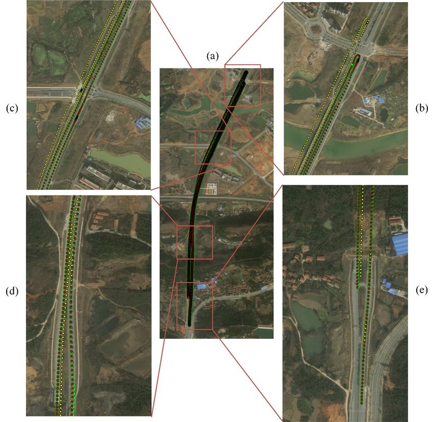
Figure 5. Comparison
Comparison results
results of our integrated model and the pure Dead Reckoning (DR) model.
Green dots
Green dots on the map are the ground truth, red dots the results
results of our integrated model, and yellow
dots
dots the
the results
resultsofofthe
theDR
DRmodel.
model.(a)(a)The
Theresults
resultsfor
forthe
thewhole
wholemeasurement
measurementtrip.
trip.(b–e)
(b–e)the
theresults forfor
results 4
specific areas.
4 specific areas.
Figure 6 shows a boxplot of the vehicle positioning error in the DR model and our system, and a
boxplot of the runtime of our system. The data for the boxplot is at 1 Hz for both the DR model and
our system. Our system’s median error was about 0.3 m while that of the DR model is about 100 m.
Moreover, the median run time of our system is 12 ms, and for all the time steps (cycles) the runtime is
less than 100 ms. Therefore, our system meets real-time requirements as the cycle is 1 s.
Figure 7 shows the time series of vehicle state errors in the DR model and our system. In Figure 7a
the DR model’s position error is increasing with time in the first half of the trip, after reaching a peak,
it keeps decreasing. However, Position Dilution of Precision (PDOP) for the DR model is reflected by
the error covariance matrix Pk in Equation (12), increasing over time. The DR model position error,
as calculated by the ground truth, decreased unexpectedly in the second half of the trip, possibly due to
random values in the EKF. Dilution of Precision (DOP) is not consistent with the error calculated from
the ground truth, nor the error calculated from the velocity and attitude. Figure 7b shows the velocity
error in the driving direction. The DR model’s velocity error is much larger than that of our system.
In Table 1, we can see that the accelerometer in SPAN-CPT is at a MEMS level, its large drift error leads
to deviation quickly during operation. However, in Figure 7d–f, errors of pitch, roll and yaw angles of
the DR model are slightly larger than those of our system, which is due to the good quality of FOG in
SPAN-CPT. As the pitch data is matched in our work, Figure 7c shows the time series of pitch data for
the DR model, our system and the ground truth. We can see that both the DR model and our system
achieved a similar pattern with the ground truth, and pitch data from our system is slightly closer to
the ground truth than the DR model. The similarity and accuracy of the pitch data from our systemRemote Sens. 2020, 12, x FOR PEER REVIEW 13 of 19
RemoteFigure 6 shows
Sens. 2020, 12, 2607a boxplot of the vehicle positioning error in the DR model and our system, 13 and a
of 18
boxplot of the runtime of our system. The data for the boxplot is at 1 Hz for both the DR model and
our system. Our system’s median error was about 0.3 m while that of the DR model is about 100 m.
benefit ourthe
Moreover, matching
medianprocess,
run timehelp find
of our a precise
system is 12estimation
ms, and forofallthe
thevehicle’s position,
time steps (cycles)and
the lead to a
runtime
positive constraint on the drift errors of the gyroscope and accelerometer in
is less than 100 ms. Therefore, our system meets real-time requirements as the cycle is 1 s.the integration model.
We can see that it is a positive recursive procedure and makes our system more robust.
Figure 6. The error of localization from the pure DR model and our integrated model, compared with
Figure 6. The
the ground error
truth of localization
from RTK-GPS, andfromthe
theruntime
pure DRofmodel and our integrated
our integrated model. model, compared with
Remote Sens. 2020, 12, x FOR PEER REVIEW 14 of 19
the ground truth from RTK-GPS, and the runtime of our integrated model.
Figure 7 shows the time series of vehicle state errors in the DR model and our system. In Figure
7a the DR model’s position error is increasing with time in the first half of the trip, after reaching a
peak, it keeps decreasing. However, Position Dilution of Precision (PDOP) for the DR model is
reflected by the error covariance matrix P k in Equation (12), increasing over time. The DR model
position error, as calculated by the ground truth, decreased unexpectedly in the second half of the
trip, possibly due to random values in the EKF. Dilution of Precision (DOP) is not consistent with the
error calculated from the ground truth, nor the error calculated from the velocity and attitude.
Figure 7b shows the velocity error in the driving direction. The DR model’s velocity error is much
larger than that of our system. In Table 1, we can see that the accelerometer in SPAN-CPT is at a
MEMS level, its large drift error leads to deviation quickly during operation. However, in Figure
7d–f, errors of pitch, roll and yaw angles of the DR model are slightly larger than those of our
system, which is due to the good quality of FOG in SPAN-CPT. As the pitch data is matched in our
work, Figure 7c shows the time series of pitch data for the DR model, our system and the ground
truth. We can see that both the DR model and our system achieved a similar pattern with the ground
truth, and pitch data from our system is slightly closer to the ground truth than the DR model. The
similarity and accuracy of the pitch data from our system benefit our matching process, help find a
precise estimation of the vehicle’s position, and lead to a positive constraint on the drift errors of the
gyroscope and accelerometer in the integration model. We can see that it is a positive recursive
procedure and makes our system more robust.
Figure 7. Time series of the errors of position, attitude and velocity for the pure DR model and our
Figure 7. Time
integrated series
model, of the errors
compared of ground
with the position,truth
attitude
fromand velocity
RTK-GPS andforSPAN-CPT.
the pure DR model and our
integrated model, compared with the ground truth from RTK-GPS and SPAN-CPT.
These results indicate that DR model is vulnerable to the biases of the gyroscope, accelerometer
These results
and odometer. Ourindicate
systemthat DR model isfor
compensates vulnerable to the
these biases bybiases of the position
integrating gyroscope, accelerometer
estimation with
and odometer.
higher accuracy Our system compensates
for improved for these biases
positioning performance. The by
FFTintegrating position estimation
and DTW processes in our workwith
are
higher accuracy
implemented forFFTW
with improved positioning
and fast performance.
DTW, furthermore, weThe FFT andoptimize
extensively DTW processes in our
their codes work
to make
are implemented
them with
even faster for FFTWcomputing.
real-time and fast DTW, furthermore,
Our system deliverswe extensively
high optimize
performance their codes
and efficiency withto
a
make them
median even
position faster
error form real-time
of 0.3 computing.
and a median Our
runtime of system delivers high performance and
12 ms.
efficiency with a median position error of 0.3 m and a median runtime of 12 ms.
4. Discussion
In our system, we use a TSS-matching model in a DTW algorithm to find the possible positions
of a vehicle. We choose n positions where the DTW distance is minima instead of the smallestRemote Sens. 2020, 12, 2607 14 of 18
4. Discussion
In our system, we use a TSS-matching model in a DTW algorithm to find the possible positions of
a vehicle. We choose n positions where the DTW distance is minima instead of the smallest distance of
Dk in Algorithm 2. Then through the constraint in Algorithm 2, we find the best positioning estimation
from n minima. The smallest DTW distance means that its corresponding subsequence on the reference
map matches our calculated pitch subsequence the best. But it may not be the right position. This is
reasonable because compared with other applications of TSS matching, amplitudes of pitch values are
small, pitch values are vulnerable to disturbances, and for flat road or straight slope the pitch curve
may have less features, so subsequences of pitch data at different positions on the reference map may
have similar patterns and have similar DTW distances. In this situation, we need an extra constraint,
as in Algorithm 2, to find the right positioning estimation. Figure 8 supports our assumption by
presenting the position error of using the smallest DTW distance of Dk instead of minima in our system.
e Sens. 2020, 12,Wex FOR
can seePEER REVIEW
that there is a wrong positioning estimation at around 7 min. The error caused by this 1
erroneous positioning estimation accumulates and affects all cycles afterwards.
Figure 8. Boxplot and time series of the position error of the integrated model using smallest
Figure 8. BoxplotDTW distance.
and time series of the position error of the integrated model using smallest DTW
distance. We also test how these parameters affect the performances of our system by control variates
method. A series of tests named Testk, k = 1, 2, ...5 are implemented with parameters values shown
in Table 3. Parameter values of the control group are from Table 2. The parameter values with gray
We also testbackground
how these parameters
are different affect thevalues
from the corresponding performances of our
in the control group. system
Note that dthre2 is by
not control var
hod. A seriestested, because
of tests we think itTest
named is large = 1, 2,...5
k , kenough in our work. Figure 9 shows the position
are implemented witherror and runtime values show
parameters
of the tests and the control group. We can see that if we increase dw from 10 to 20 m, the boxplot of the
e 3. Parameter values
position of the
error slightly control
changes, but thegroup are from
runtime increases a lot.dTable 2. mean
w increases Thethat
parameter
the number ofvalues with
k
from the corresponding values in the control group. Note that dthre 2 i
road points Y in Equation (15) increases and the iteration in the loop in Algorithm 1 also increases,
ground are different
which increases time consumption. Even though dw is increased from 10 to 20 m, considering our
d, because we think
system’s it is error
positioning largewhichenough
is less thanin our
2 m, work.
the search Figure
window 910shows
(−10 m, m) is largethe
enoughposition error
to find the right position. Therefore, Test1 results in a similar boxplot of position error with the
me of the tests
controland the control group. We can see that if we increase d w from 10 to 20 m
group.
lot of the position error slightly changes, but the runtime increases a lot. d w increases m
the number of road points Y k in Equation (15) increases and the iteration in the loo
rithm 1 also increases, which increases time consumption. Even though d w is increased fro
m, considering our system’s positioning error which is less than 2 m, the search windowdistance.
We also test how these parameters affect the performances of our system by control variates
method. A series of tests named Testk , k = 1, 2,...5 are implemented with parameters values shown in
Table 3. Parameter values of the control group are from Table 2. The parameter values with gray
Remote Sens. 2020, 12, 2607 15 of 18
background are different from the corresponding values in the control group. Note that dthre 2 is not
tested, because we think it is large enough in our work. Figure 9 shows the position error and
Table
runtime Predefined
of 3.the tests andparameters andgroup.
the control their values for the
We can seefive testing
that if weexperiments
increase dand the control group.
w from 10 to 20 m, the
boxplot of the position error slightly
Parameter dw changes,
fc but the
td runtime increases
dthre1 a lot. d wn increases mean
dthre2
k
that the number ofTest1
road points 20Ym in Equation
8 Hz (15)
2 s increases
5 m and 0.5
themiteration8 in the loop in
Algorithm 1 also increases,
Test2 which increases
10 m time
5 Hz consumption.
2s Even 0.5 m d w is increased
5 m though 8 from 10
to 20 m, consideringTest3
our system’s10 m 8 Hzerror which
positioning 5s 5 mthan 20.5m,
is less mthe search
8 window (−10
Test4 10 m 8 Hz 2s 10 m 0.5 m 8
m, 10 m) is large enough
Test5
to find the
10 m
right position.
8 Hz
Therefore,
2s 5m
Test1 results
0.5 m
in a similar
4
boxplot of
position error with the control
Control Group group.
10 m 8 Hz 2s 5m 0.5 m 8
Figure 9. Position error and runtime for the five testing experiments and the control group.
Figure 9. Position error and runtime for the five testing experiments and the control group.
In Test2, the cutoff frequency fc in the low-pass filter in Algorithm 2 decreases from 8 to 5 Hz; from
Figure 9 we can see that the positioning result is slightly worse than the control group, and the running
time is almost the same. fc has no effect on runtime. Lower fc means a smoother pitch subsequence,
but less small features, which is not good for finding the best position estimation.
From Figure 1 and Equation (14), we can see that td controls the length of the pitch subsequence.
In Test3, td increases from 2 to 5 s, which means more pitch data are involved in the matching procedure
so that the DTW algorithm takes more time. The positioning accuracy is similar to that of the control
group, which means that pitch data in the duration of 2 s are enough to find the best position estimation.
In Figure 1, dthre1 is a distance threshold; if the accumulated distance that the vehicle moves
within td is less than dthre1 , the navigation state from the DR model is assumed to be the vehicle’s
final state at the current time step. This constraint is for low speed situations, like waiting for traffic
lights or obstacle avoidance. In Figure 3, we can see that the vehicle stops twice, and the second stop
lasts for about 1 min. During these situations, the vehicle uses the DR model directly to calculate its
navigation state. If dthre1 is increased from 5 to 10 m (the situation lasts for longer for the vehicle),
our integration model works less, and the vehicle takes the direct output from the DR model in more
cycles. From Figure 9, we can see that in Test4 there is a larger position error and the runtime is similar
to the that of the control group.
From Algorithm 2, we can see that the number n of minima has a direct effect on the choice
of possible position estimations in matrix Mk . Larger n means more possible estimations using the
constraint in Algorithm 2 to obtain the best estimation mk . In Test 5, we decrease n from 8 to 4.Remote Sens. 2020, 12, 2607 16 of 18
From Figure 9, we can see that 8 minima can produce a more accurate position estimation and n has a
very limited effect on runtime.
5. Conclusions
This paper proposed an integrated model for real-time localization. This integrated model deploys
a DR model and a DTW algorithm. The DR model calculates the vehicle’s navigation state (position,
velocity and attitude) by IMU and odometer. However, the DR model is vulnerable to the drift error of
gyroscope and accelerometer in the IMU and the accumulated error of odometer. Using the prediction
of the vehicle’s navigation state from the DR model, we take advantage of R-Tree to find the closest
road point in the reference terrain map efficiently. Given a search window centering on this road point,
we match our calculated pitch data over a period with the pitch data stored in the reference map using
DTW algorithm to find the best-fit position estimation. This position estimation is integrated with
the DR model by EKF to get final navigation state. The integration constrains IMU drift error and
accumulated odometer error for improved positioning accuracy. Field experiments were conducted
to test the integrated system, the terrain map covered a route more than 6 km and the measurement
trip lasted for more than 10 min. In our work, we used a high-performance MEMS-level IMU sensor
which helped the DR system provide good estimations of positions. In the future, we will try low-cost
MEMS-level IMU sensors in our system to make our system more practical. Experimental results show
that our integrated system can accurately (mean position error: 0.3 m) and efficiently (median runtime:
12 ms) localize the vehicle.
Author Contributions: Conceptualization, H.Z. and W.L.; methodology, H.Z.; software, W.L.; validation,
C.Q. and H.Z.; writing H.Z.; supervision, B.L. All authors have read and agreed to the published version of
the manuscript.
Funding: This work was supported in part by the National Key Research and Development Program of China
under Grant 2018YFB1600600, in part by the National Natural Science Foundation of China under Grant 41801377,
41801344 and in part by National Natural Science Foundation of China under Grant U1764262.
Conflicts of Interest: The authors declare no conflict of interest.
References
1. Wanninger, L.; Beer, S. BeiDou satellite-induced code pseudorange variations: Diagnosis and therapy.
GPS Solut. 2015, 19, 639–648. [CrossRef]
2. Li, X.; Ge, M.; Dai, X.; Ren, X.; Fritsche, M.; Wickert, J.; Schuh, H. Accuracy and reliability of multi-GNSS
real-time precise positioning: GPS, GLONASS, BeiDou, and Galileo. J. Geod. 2015, 89, 607–635. [CrossRef]
3. Hide, C.; Moore, T.; Smith, M. Adaptive Kalman filtering for low-cost INS/GPS. J. Navig. 2003, 56, 143–152.
[CrossRef]
4. Ahmed, H.; Tahir, M. Terrain-based vehicle localization using low cost MEMS-IMU sensors. In Proceedings
of the 2016 IEEE 83rd Vehicular Technology Conference (VTC Spring), Nanjing, China, 15–18 May 2016;
pp. 1–5.
5. Tin Leung, K.; Whidborne, J.F.; Purdy, D.; Dunoyer, A. A review of ground vehicle dynamic state estimations
utilising GPS/INS. Veh. Syst. Dyn. 2011, 49, 29–58. [CrossRef]
6. Malvezzi, M.; Vettori, G.; Allotta, B.; Pugi, L.; Ridolfi, A.; Rindi, A. A localization algorithm for railway
vehicles based on sensor fusion between tachometers and inertial measurement units. Proc. Inst. Mech. Eng.
Part F J. Rail Rapid Transit 2014, 228, 431–448. [CrossRef]
7. Georgy, J.; Karamat, T.; Iqbal, U.; Noureldin, A. Enhanced MEMS-IMU/odometer/GPS integration using
mixture particle filter. GPS Solut. 2011, 15, 239–252. [CrossRef]
8. Levinson, J.; Montemerlo, M.; Thrun, S. Map-based precision vehicle localization in urban environments.
Robot. Sci. Syst. 2007, 4, 1.
9. Se, S.; Lowe, D.; Little, J. Vision-based mobile robot localization and mapping using scale-invariant features.
In Proceedings of the Proceedings 2001 ICRA. IEEE International Conference on Robotics and Automation
(Cat. No. 01CH37164), Seoul, Korea, 21–26 May 2001; pp. 2051–2058.You can also read