MULTILAYER-HYSEA MODEL VALIDATION FOR LANDSLIDE-GENERATED TSUNAMIS - PART 2: GRANULAR SLIDES
←
→
Page content transcription
If your browser does not render page correctly, please read the page content below
Nat. Hazards Earth Syst. Sci., 21, 791–805, 2021
https://doi.org/10.5194/nhess-21-791-2021
© Author(s) 2021. This work is distributed under
the Creative Commons Attribution 4.0 License.

Multilayer-HySEA model validation for landslide-generated
tsunamis – Part 2: Granular slides
Jorge Macías1 , Cipriano Escalante1,a , and Manuel J. Castro1
1 Departamento     de Análisis Matemático, Estadística e Investigación Operativa y Matemática Aplicada,
Facultad de Ciencias, Universidad de Málaga, 29080 Málaga, Spain
a current affiliation: Departamento de Matemáticas, Campus de Rabanales, Universidad de Córdoba, 14071 Córdoba, Spain

Correspondence: Jorge Macías (jmacias@uma.es)

Received: 22 May 2020 – Discussion started: 15 September 2020
Revised: 16 January 2021 – Accepted: 18 January 2021 – Published: 26 February 2021

Abstract. The final aim of the present work is to pro-           be found in the companion paper. Then, results for the three
pose a NTHMP-benchmarked numerical tool for landslide-           NTHMP benchmark problems dealing with tsunamis gener-
generated tsunami hazard assessment. To achieve this, the        ated by granular slides are presented with a description of
novel Multilayer-HySEA model is validated using labora-          each benchmark problem.
tory experiment data for landslide-generated tsunamis. In
particular, this second part of the work deals with granular
slides, while the first part, in a companion paper, consid-
ers rigid slides. The experimental data used have been pro-      1   Introduction
posed by the US National Tsunami Hazard and Mitigation
Program (NTHMP) and were established for the NTHMP               Following the introduction of the companion paper Macías
Landslide Benchmark Workshop, held in January 2017 at            et al. (2021), a landslide tsunami model benchmarking and
Galveston (Texas). Three of the seven benchmark problems         validation workshop was held on 9–11 January 2017 in
proposed in that workshop dealt with tsunamis generated by       Galveston, TX. This workshop was organized on behalf of
rigid slides and are collected in the companion paper (Macías    the NOAA National Weather Service’s National Tsunami
et al., 2021). Another three benchmarks considered tsunamis      Hazard Mitigation Program (NTHMP) Mapping and Mod-
generated by granular slides. They are the subject of the        eling Subcommittee (MMS) with the expected outcome be-
present study. The seventh benchmark problem proposed the        ing to (i) develop a set of community-accepted benchmark
field case of Port Valdez, Alaska, 1964 and can be found in      tests for validating models used for landslide tsunami gen-
Macías et al. (2017). In order to reproduce the laboratory ex-   eration and propagation in NTHMP inundation mapping
periments dealing with granular slides, two models need to       work; (ii) develop workshop documentation and a web-based
be coupled: one for the granular slide and a second one for      repository, for benchmark data, model results, and work-
the water dynamics. The coupled model used consists of a         shop documentation, results, and conclusions; and (iii) pro-
new and efficient hybrid finite-volume–finite-difference im-     vide recommendations as a basis for developing best-practice
plementation on GPU architectures of a non-hydrostatic mul-      guidelines for landslide tsunami modeling in NTHMP work.
tilayer model coupled with a Savage–Hutter model. To intro-         A set of seven benchmark tests was selected (Kirby et al.,
duce the multilayer model more fluidly, we first present the     2018). The selected benchmarks were taken from a sub-
equations of the one-layer model, Landslide-HySEA, with          set of available laboratory data sets for solid slide exper-
both strong and weak couplings between the fluid layer and       iments (three of them) and deformable slide experiments
the granular slide. Then, a brief description of the multi-      (another three) that included both submarine and subaerial
layer model equations and the numerical scheme used is in-       slides. Finally, a benchmark based on a historic field event
cluded. The dispersive properties of the multilayer model can    (Valdez, AK, 1964) closed the list of proposed benchmarks.
                                                                 The EDANYA group (https://www.uma.es/edanya, last ac-

Published by Copernicus Publications on behalf of the European Geosciences Union.
792 J. Macías et al.: Multilayer-HySEA model validation for landslide-generated tsunamis – Part 2
cess: 21 February 2021) from the University of Malaga par- material. Well-controlled 2D glass bead experiments were re-
ticipated in the aforementioned workshop, and the numerical ported and modeled by Grilli et al. (2017) using the model of
codes Multilayer-HySEA and Landslide-HySEA were used Kirby et al. (2016).
to produce our modeled results. We presented numerical re- The benchmark problems performed in the present work
sults for six out of the seven benchmark problems proposed, are based on the laboratory experiments of Kimmoun and
including the field case (Macías et al., 2017). The sole bench- Dupont (see Grilli et al., 2017) for BP4, Viroulet et al. (2014)
mark we did not perform at the time was BP6, for which nu- for BP5, and Mohammed and Fritz (2012) for BP6. The ba-
merical results are included here. sic reference for these three benchmarks, but also the three
The present work aims at showing the numerical re- related to solid slides and the Alaska field case, all of them
sults obtained with the Multilayer-HySEA model in the proposed by the NTHMP, is Kirby et al. (2018). That is a key
framework of the validation effort described above for reference for readers interested in the benchmarking initia-
the case of granular-slide-generated tsunamis for the com- tive which the present work is based on.
plete set of the three benchmark problems proposed by the
NTHMP. However, the ultimate goal of the present work is
to provide the tsunami community with a numerical tool, 2 The Landslide-HySEA model for granular slides
tested and validated meeting the defined criteria for the
First we consider the Landslide-HySEA model, applied in
NTHMP, for landslide-generated tsunami hazard assessment.
Macías et al. (2015) and González-Vida et al. (2019), which
This NTHMP acceptance has already been achieved by the
for the case of one-dimensional domains reads
Tsunami-HySEA model for the case of earthquake-generated
tsunamis (Macías et al., 2017, 2020a, c). ∂t h + ∂x (hu) = 0,
Fifteen years ago, at the beginning of the century, solid
∂ (hu) + ∂ hu 2 + 1 gh2 − gh∂ (H − z )
t x x s
2
block landslide modeling challenged researchers and was
= na (us − u) ,
undertaken by a number of authors (see companion paper, (1)
Macías et al., 2021, for references), and laboratory experi-
∂t zs + ∂x (zs us) = 0,
∂t (zs us ) + ∂x zs u2s + 12 g(1 − r)zs2
ments were developed for those cases and for tsunami model
benchmarking. In contrast, some early models (e.g., Hein-
= gzs ∂x ((1 − r)H − rη) − rna (us − u) + τP ,
rich, 1992; Harbitz et al., 1993; Rzadkiewicz et al., 1997;
Fine et al., 1998) and a number of more recent models have where g is the gravity acceleration (g = 9.81 m s−2 ); H (x) is
simulated tsunami generation by deformable slides, based the non-erodible (does not evolve in time) bathymetry mea-
either on depth-integrated two-layer model equations or on sured from a given reference level; zs (x, t) represents the
solving more complete sets of equations in terms of fea- thickness of the layer of granular material at each point x at
tured physics (dispersive, non-hydrostatic, Navier–Stokes). time t; h(x, t) is the total water depth; η(x, t) denotes the free
Examples include solutions of 2D or 3D Navier–Stokes surface (measured form the same fixed reference level used
equations to simulate subaerial or submarine slides mod- for the bathymetry, for example, the mean sea surface) and
eled as dense Newtonian or non-Newtonian fluids (Ataie- is given by η = h + zs − H ; u(x, t) and us (x, t) are the av-
Ashtiani and Shobeyri, 2008; Weiss et al., 2009; Abadie eraged horizontal velocity for the water and for the granular
et al., 2010, 2012; Horrillo et al., 2013), flows induced by material, respectively; and r = ρρ12 is the ratio of densities be-
sediment concentration (Ma et al., 2013), or fluid or gran- tween the ambient fluid and the granular material. The term
ular flow layers penetrating or failing underneath a 3D wa- na (us − u) parameterizes the friction between the fluid and
ter domain – for example, the two-layer models of Macías the granular layer. Finally, the term τP (x, t) represents the
et al. (2015) or González-Vida et al. (2019), where a fully friction between the granular slide and the non-erodible bot-
coupled non-hydrostatic SW/Savage–Hutter model is used, tom surface. It is parameterized as in Pouliquen and Forterre
or the model used in Ma et al. (2015) and Kirby et al. (2016), (2002), and it is described in the next section.
in which the upper water layer is modeled with the non- System Eq. (1) presents the difficulty of considering the
hydrostatic σ -coordinate 3D model NHWAVE (Ma et al., complete coupling between sediment and water, including
2012). For a more comprehensive review of recent modeling the corresponding coupled pressure terms. That makes its
work, see Yavari-Ramshe and Ataie-Ashtiani (2016). A num- numerical approximation more complex. Moreover, it also
ber of recent laboratory experiments have modeled tsunamis makes it difficult to consider its natural extension to non-
generated by subaerial landslides composed of gravel (Fritz hydrostatic flows.
et al., 2004; Ataie-Ashtiani and Najafi-Jilani, 2008; Heller Now, if ∂x η is neglected in the momentum equation of
and Hager, 2010; and Mohammed and Fritz, 2012) or glass the granular material, that is, the fluctuation of pressure due
beads (Viroulet et al., 2014). For deforming underwater land- to the variations of the free surface is neglected in the mo-
slides and related tsunami generation, 2D experiments were mentum equation of the granular material, then the following
performed by Rzadkiewicz et al. (1997), who used sand, and weakly coupled system could be obtained:
Ataie-Ashtiani and Najafi-Jilani (2008), who used granular
Nat. Hazards Earth Syst. Sci., 21, 791–805, 2021 https://doi.org/10.5194/nhess-21-791-2021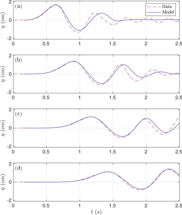
J. Macías et al.: Multilayer-HySEA model validation for landslide-generated tsunamis – Part 2 793
3 The Multilayer-HySEA model
∂t h + ∂x (hu) = 0,
S-W system ∂t (hu) + ∂x hu2 + 21 gh2 (2) The Multilayer-HySEA model implements a two-phase
−gh∂x (H − zs ) = na (us − u) , model intended to reproduce the interaction between the slide
granular material (submarine or subaerial) and the fluid. In
∂t zs + ∂x (zs us) = 0,
the present work, a multilayer non-hydrostatic shallow-water
S-H system ∂t (zs us ) + ∂x zs u2s + 21 g(1 − r)zs2 (3)
model is considered for modeling the evolution of the am-
−g(1 − r)zs ∂x H = −rna (us − u) + τP ,
bient water (see Fernández-Nieto et al., 2018), and for sim-
where the first system is the standard one-layer shallow- ulating the kinematics of the submarine/subaerial landslide
water system and the second one is the one-layer reduced- the Savage–Hutter model (Eq. 3) is used. The coupling be-
gravity Savage–Hutter model (Savage and Hutter, 1989) that tween these two models is performed through the boundary
takes into account that the granular landslide is underwater. conditions at their interface. The parameter r represents the
Note that the previous system could be also adapted to sim- ratio of densities between the ambient fluid and the granular
ulate subaerial/submarine landslides by a suitable treatment material (slide liquefaction parameter). Usually
of the variation of the gravity terms. Under this formulation,
it is now straightforward to improve the numerical model for ρf
the fluid phase by including non-hydrostatic effects. r= , ρb = (1 − ϕ)ρs + ϕρf , (4)
ρb
In the present study, the governing equations of the land-
slide motion are derived in Cartesian coordinates. In some
cases where steep slopes are involved, landslide models where ρs stands for the typical density of the granular ma-
based on local coordinates allow representing the slide mo- terial, ρf is the density of the fluid (ρs > ρf ), both con-
tion better. However, when general topographies are consid- stant, and ϕ represents the porosity (0 ≤ ϕ < 1). In the cur-
ered and not only simple geometries, landslide models based rent work, the porosity, ϕ, is supposed to be constant in space
on local coordinates also introduce some difficulties on the and time, and, therefore, the ratio r is also constant. This ra-
final numerical model and on its implementation compromis- tio ranges from 0 to 1 (i.e., 0 < r < 1) and, even on a uniform
ing, at the same time, the computational efficiency of the nu- material, is difficult to estimate as it depends on the porosity
merical model. Here, we focus on the hydrodynamic compo- (and ρf and ρs are also supposed to be constant). Typical
nent of the system, and that is one of the reasons for choosing values for r are in the interval [0.3, 0.8].
a simple landslide model based on Cartesian coordinates. Of
course, the strategies presented here can also be adapted for The fluid model
more sophisticated landslide models. For example, in Garres-
Díaz et al. (2021) a non-hydrostatic model for the hydrody- The ambient fluid is modeled by a multilayer non-hydrostatic
namic part that is similar to the one presented here for the shallow-water system (Fernández-Nieto et al., 2018) to ac-
case of a single layer was introduced. In the work mentioned count for dispersive water waves. The model considered,
above, the authors study the influence of coupling the hy- that is obtained by a process of depth-averaging of the Euler
drodynamic model with a granular model that is derived in equations, can be interpreted as a semi-discretization with re-
both reference systems: Cartesian and local coordinates. The spect to the vertical coordinate. In order to take into account
front positions calculated with the Cartesian model progress dispersive effects, the total pressure is decomposed into the
faster, and, after some time, they are slightly ahead com- sum of hydrostatic and non-hydrostatic components. In this
pared with the local coordinate model solution (see, for in- process, the horizontal and vertical velocities are supposed
stance, Fig. 4 in Garres-Díaz et al., 2021). This is due to to have constant vertical profiles. The resulting multilayer
the fact that the Cartesian model uses the horizontal veloc- model admits an exact energy balance, and when the number
ity instead of the velocity tangent to the topography. In any of layers increases, the linear dispersion relation of the linear
case, the differences between the two models are not very no- model converges to that of Airy’s theory. Finally, the model
ticeable. A granular slide model based on local coordinates proposed in Fernández-Nieto et al. (2018) can be written in
might give better results. However, when introducing a non- compact form as
hydrostatic pressure, the model is closer to a 3D solver. In
such a case, the influence on the reference coordinate system
barely exists. That is the reason why in Garres-Díaz et al.
∂t h + ∂x (hu) = 0,
2 + 1 gh2 − gh∂ (H − z )
∂ (hu ) + ∂ hu
(2021) both non-hydrostatic models based on different coor-
t α x α 2 x s
dinate systems show similar results. In any case, although on +uα+1/2 0α+1/2 − uα−1/2 0α−1/2
the present work we focus on the hydrodynamic part, it can = −h (∂x pα + σα ∂z pα ) − τα (5)
be observed on the benchmark tests that the numerical results ∂t (hwα ) + ∂x (huα wα ) + wα+1/2 0α+1/2
are in very good agreement with the laboratory-measured −wα−1/2 0α−1/2 = −h∂z pα ,
data, despite the simple landslide model chosen here.
∂x uα−1/2 + σα−1/2 ∂z uα−1/2 + ∂z wα−1/2 = 0,
https://doi.org/10.5194/nhess-21-791-2021 Nat. Hazards Earth Syst. Sci., 21, 791–805, 2021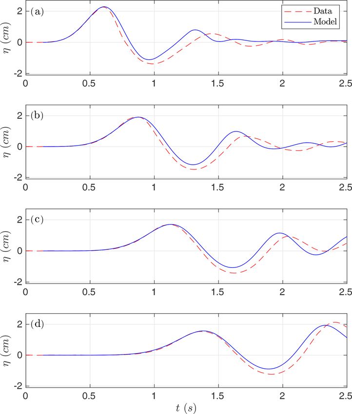
794                         J. Macías et al.: Multilayer-HySEA model validation for landslide-generated tsunamis – Part 2

Figure 1. Schematic diagram describing the multilayer system.

for α ∈ {1, 2, . . . , L}, with L the number of layers and where   Here we suppose that 01/2 = 0L+1/2 = 0; this means that
the following notation has been used:                              there is no mass transfer through the sea floor or the water
                                                                   free surface. In order to close the system, the boundary con-
          1
fα+1/2 =    (fα+1 + fα ) ,                                         dition
          2
              1                                                    pL+1/2 = 0
∂z fα+1/2 =      (fα+1 − fα ) ,
            h1s
                                                                   is imposed at the free-surface and the boundary conditions
where f denotes one of the generic variables of the system,
i.e., u, w, and p; 1s = 1/L and, finally,                          u0 = 0, w0 = −∂t (H − zs )

σα = ∂x (H − zs − h1s(α − 1/2)) ,                                  are imposed at the bottom. The last two conditions enter into
σα−1/2 = ∂x (H − zs − h1s(α − 1)) .                                the incompressibility relation for the lowest layer (α = 1),
                                                                   given by
   Figure 1 shows a schematic picture of the model configura-
tion, where the total water height h is decomposed along the       ∂x u1/2 + σ1/2 ∂z u1/2 + ∂z w1/2 = 0.
vertical axis into L ≥ 1 layers. The depth-averaged velocities
                                                                   It should be noted that both models, the hydrodynamic model
in the x and z directions are written as uα and wα , respec-
                                                                   described here and the morphodynamic model described in
tively. The non-hydrostatic pressure at the interface zα+1/2
                                                                   the next subsection, are coupled through the unknown zs ,
is denoted by pα+1/2 . The free-surface elevation measured
                                                                   which, in the case of the model described here, is present in
from a fixed reference level (for example the still-water level)
                                                                   the equations and in the boundary condition (w0 = −∂t (H −
is written as η and η = h − H + zs , where again H (x) is the
                                                                   zs )).
unchanged non-erodible bathymetry measured from the same
                                                                      Some dispersive properties of system Eq. (5) were orig-
fixed reference level. τα = 0 for α > 1, and τ1 is given by
                                                                   inally studied in Fernández-Nieto et al. (2018). Moreover,
τ1 = τb − na (us − u1 ) ,                                          for a better-detailed study on the dispersion relation (such as
                                                                   phase velocity, group velocity, and linear shoaling) the reader
where τb stands for an classical Manning-type parameteri-          is referred to the companion paper Macías et al. (2021).
zation for the bottom shear stress and, in our case, is given         Along the derivation of the hydrodynamic model pre-
by                                                                 sented here, the rigid-lid assumption for the free surface of
                                                                   the ambient fluid is adopted. This means that pressure vari-
           n2
τb = gh        u1 |u1 |,                                           ations induced by the fluctuation on the free surface of the
          h4/3                                                     ambient fluid over the landslide are neglected.
and na (us − u1 ) accounts for the friction between the fluid
and the granular layer. The latest two terms are only present      The landslide model
at the lowest layer (α = 1). Finally, for α = 1, . . . , L − 1,
                                                                   The 1D Savage–Hutter model used and implemented in the
0α+1/2 parameterizes the mass transfer across interfaces, and
                                                                   present work is given by system Eq. (3). The friction law τP
those terms are defined by
                                                                   (Pouliquen and Forterre, 2002) is given by the expression
             L                          L
                                                                                         u2s
             X                        X
0α+1/2 =            ∂x h1s uβ − u , u =   1suα .
                                                                   τP = −g(1 − r)µzs          ,
            β=α+1                            α=1                                        |us |

Nat. Hazards Earth Syst. Sci., 21, 791–805, 2021                                    https://doi.org/10.5194/nhess-21-791-2021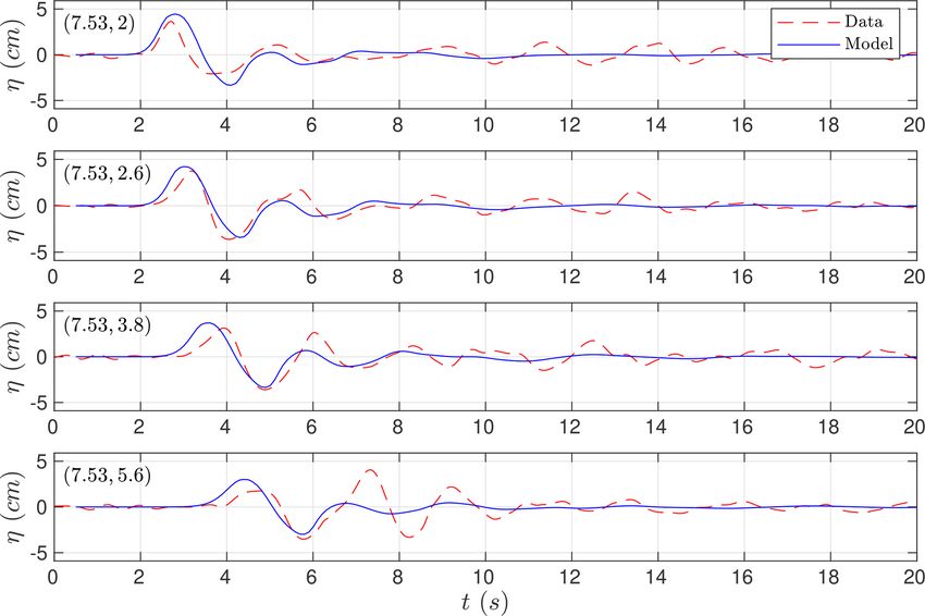
J. Macías et al.: Multilayer-HySEA model validation for landslide-generated tsunamis – Part 2 795
where µ is a constant friction coefficient with a key role, as it Analogously, the multilayer non-hydrostatic shallow-water
controls the movement of the landslide. Usually µ is given by system Eq. (5) can also be expressed in a similar way:
the Coulomb friction law as the simpler parameterization that
can be used in landslide models. However, it is well known ∂t Uf + ∂x Ff Uf + Bf Uf ∂x Uf
that a constant friction coefficient does not allow us to re- = Gf (U )∂x(H − zs ) + TNH −Sf Uf , (7)
B Uf , Uf x , H, Hx , zs , (zs )x = 0,
produce steady uniform flows over rough beds observed in
the laboratory for a range of inclination angles. To reproduce
these flows, in Pouliquen and Forterre (2002), the authors in- where
troduce an empirical friction coefficient µ that depends on
h
hu
the norm of the mean velocity us , on the thickness zs of the hu1 hu2 + 1 gh2
granular layer, and on the Froude number F r = √ugzs s . The
..
1
..
2
. .
friction law is given by
Uf = hu , F U 2 1 2
L f f = huL + 2 gh ,
µ (zs , us ) = hw1 hu1 w1
γ . ..
..
(
µstart (zs ) + Fβr
µstop (zs ) − µstart (zs ) , for F r < β, .
µstop (zs ) , for β ≤ F r, hwL huL wL
0
with gh
zs
..
.
µstart (zs ) = tan (δ3 ) + (tan (δ2 ) − tan (δ1 )) exp − ,
ds
Gf Uf = gh ,
zs β 0
µstop (zs ) = tan (δ1 ) + (tan (δ2 ) − tan (δ1 )) exp − ,
..
ds F r .
where ds represents the mean size of grains. β = 0.136 and 0
γ = 10−3 are empirical parameters. tan(δ1 ) and tan(δ2 ) are
and Bf (Uf )∂x (Uf ) contains the non-conservative products
the characteristic angles of the material, and tan(δ3 ) is other
involving the momentum transfer across the interfaces, and,
friction angle related to the behavior when starting from
finally, Sf (Uf ) represents the friction terms,
rest. This law has been widely used in the literature (see,
e.g., Brunet et al., 2017).
0
Note that the slide model can also be adapted to simulate u3/2 03/2
subaerial landslides. The presence of the term (1 − r) in the
u5/3 05/2 − u3/2 03/2
definition of the Pouliquen–Forterre friction law is due to the
..
buoyancy effects, which must be taken into account only in
.
the case that the granular material layer is submerged in the Bf Uf ∂x Uf =
−uL−1/2 0L−1/2 ,
fluid. Otherwise, this term must be replaced by 1.
w3/2 03/2
w5/3 05/2 − w3/2 03/2
..
4 Numerical solution method .
−wL−1/2 0L−1/2
System Eq. (3) can be written in the following compact form:
0
τb − na (us − u1 )
∂t Us + ∂x Fs (Us ) = Gs (Us ) ∂x H − Ss (Us ) , (6)
Sf Uf =
0 .
..
being
.
0
zs zs us
Us = , Fs (Us ) = ,
us zs zs u2s + 12 g(1 − r)zs2 The non-hydrostatic corrections in the momentum equations
are given by
0
Gs (Us ) = ,
g(1 − r)zs
0
Ss (Us ) = .
−rna (us − u) + τP
https://doi.org/10.5194/nhess-21-791-2021 Nat. Hazards Earth Syst. Sci., 21, 791–805, 2021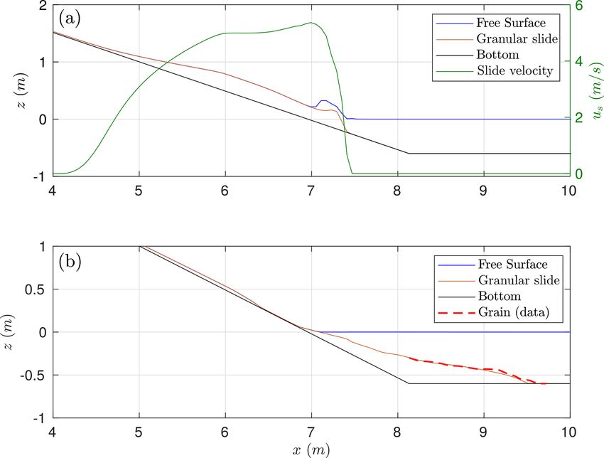
796 J. Macías et al.: Multilayer-HySEA model validation for landslide-generated tsunamis – Part 2
et al., 2018a, b). For the discretization of the Coulomb fric-
tion term, we refer the reader to Fernández-Nieto et al.
TNH = TNH h, hx , H, Hx , zs , (zs )x , p, px
(2008).
0
h (∂x p1 + σ1 ∂z p1 ) The resulting numerical scheme is well balanced for the
..
water-at-rest stationary solution and is linearly L∞ stable un-
.
der the usual CFL condition related to the hydrostatic system.
= − h (∂x pL + σL ∂z pL )
, It is also worth mentioning that the numerical scheme is pos-
h∂z p 1
itive preserving and can deal with emerging topographies.
.. Finally, its extension to 2D is straightforward. For dealing
.
with numerical experiments in 2D regions, the computational
h∂z pL domain must be decomposed into subsets with a simple ge-
and, finally, the operator related with the incompressibility ometry, called cells or finite volumes. The 2D numerical al-
condition at each layer is given by gorithm for the hydrodynamic hyperbolic component of the
coupled system is well suited to be parallelized and imple-
B Uf , Uf x , H, Hx , zs , (zs )x mented in GPU architectures, as is shown in Castro et al.
(2011). Nevertheless, a standard treatment of the elliptic part
∂x u1/2 + σ1/2 ∂z u1/2 + ∂z w1/2
.. of the system does not allow the parallelization of the al-
= .
. gorithms. The method used here and proposed in Escalante
∂x uL−1/2 + σL−1/2 ∂z uL−1/2 + ∂z wL−1/2 et al. (2018a, b) makes it possible that the second step can
also be implemented on GPUs, due to the compactness of the
The discretization of systems (Eqs. 6 and 7) becomes diffi- numerical stencil and the easy and massive parallelization of
cult. In the present work, the natural extension of the numer- the Jacobi method The above-mentioned parallel GPU and
ical schemes proposed in Escalante et al. (2018a, b) is con- multi-GPU implementation of the complete algorithm results
sidered. These authors propose, describe, and use a splitting in much shorter computational times.
technique. Initially, the systems (Eqs. 6 and 7) are expressed
as the following non-conservative hyperbolic system:
5 Benchmark problem comparisons
Gs (Us ) ∂x H,
∂t Us + ∂x Fs (Us ) =
∂t Uf + ∂x Ff Uf + Bf Uf ∂x Uf = Gf Uf ∂x (H − zs ) .
(8)
This section presents the numerical results obtained with the
Both equations are solved simultaneously using a second- Multilayer-HySEA model for the three benchmark problems
order HLL (Harten–Lax–van Leer), positivity-preserving, dealing with granular slides and the comparison with the
and well-balanced, path-conservative finite-volume scheme measured lab data for the generated water waves. In particu-
(see Castro and Fernández-Nieto, 2012) and using the same lar, BP4 deals with a 2D submarine granular slide, BP5 with
time step. The synchronization of time steps is performed a 2D subaerial slide, and BP6 with a 3D subaerial slide. The
by taking into account the Courant–Friedrichs–Lewy (CFL) description of all these benchmarks can be found in LTMBW
condition of the complete system Eq. (8). A first-order esti- (2017) and Kirby et al. (2018). In this paper, all units, unless
mation of the maximum of the wave speed for system Eq. (8) otherwise indicated, will be expressed in the SI (International
is the following: System of Units) units.
The model parameters required in each simulation are
p p
λmax = max |us | + (g(1 − r)zs , |u| + gh . g, r, na , nm , ds , δi , β, and γ .
Then, the non-hydrostatic pressure corrections The parameters g, r, nm , and ds are related to physical set-
p1/2 , · · ·, pL−1/2 at the vertical interfaces are computed tings given in each experiment. β and γ are empirical param-
from eters that were chosen as in the seminal paper of Pouliquen
and Forterre (2002).
∂t Uf = TNH h, hx , H, Hx , zs , (z
s )x , p, px , The friction angles δ1 and δ2 are characteristic angles of
B Uf , Uf x , H, Hx , zs , (zs )x = 0,
the material, and δ3 is related to the behavior of the slide mo-
which requires the discretization of an elliptic operator that is tion when starting from the rest. Thus, the values of these an-
done using standard second-order central finite differences. gles strongly depend on the granular material. They were ad-
This results in a linear system than in our case is solved justed within a range of feasible values according to the refer-
using an iterative scheduled Jacobi method (see Adsuara ences (Brunet et al., 2017; Mangeney et al., 2007; Pouliquen
et al., 2016). Finally, the computed non-hydrostatic correc- and Forterre, 2002):
tions are used to update the horizontal and vertical momen- δ1 ∈ [1, 22◦ ], δ2 ∈ [11, 34◦ ], δ3 ∈ [3, 23◦ ].
tum equations at each layer, and, at the same time, the fric-
tions Ss (Us ) and Sf (Uf ) are also discretized (see Escalante In the present paper we have used the values
Nat. Hazards Earth Syst. Sci., 21, 791–805, 2021 https://doi.org/10.5194/nhess-21-791-2021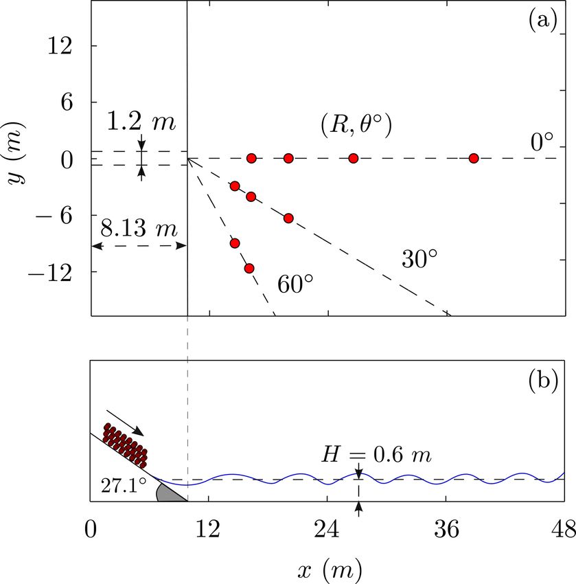
J. Macías et al.: Multilayer-HySEA model validation for landslide-generated tsunamis – Part 2 797
δ1 = 6◦ , δ2 ∈ [17, 30◦ ], δ3 = 12◦
for the three benchmark problems, which is consistent with
the values found in the literature. As noted in Mangeney et al.
(2007), in general for real problems involving complex rhe-
ologies, smaller values of these parameters δi should be em-
ployed.
With regard to the sensitivity of the model to parame- Figure 2. BP4 sketch showing the longitudinal cross section of the
ter variation, an appropriate sensitivity analysis can be per- IRPHE’s precision tank. The figure shows the location of the plane
formed, as is done in González-Vida et al. (2019). How- slope, the sluice gate, and the four gages (WG1–WG4).
ever, the aim of the present work was to prove if the non-
hydrostatic model coupled with the granular model was able
to accurately reproduce the three benchmarks considered. The one-dimensional domain [0, 6] is discretized with
Regarding the parameter denoting the buoyancy effect, for 1x = 0.005 m, and wall boundary conditions are imposed.
field cases, r = 0.5 is usually taken, and then the parameter The simulated time is 10 s. The CFL number was set to 0.5,
is eventually adjusted based on available field data. In gen- and model parameters take the following values:
eral, the complexity of the rheology introduces a difficulty
g = 9.81, r = 0.78, na = 0.2, nm = 10−3 ,
that is always present on the modeling as well as on the ad-
justment of the parameters. Moreover, the more sophisticated ds = 7 × 10⁻³ , δ1 = 6◦ , δ2 = 17◦ , δ3 = 12◦ ,
the model is (considering, for example, the rheology of the β = 0.136, γ = 10−3 .
material), more input data will be required.
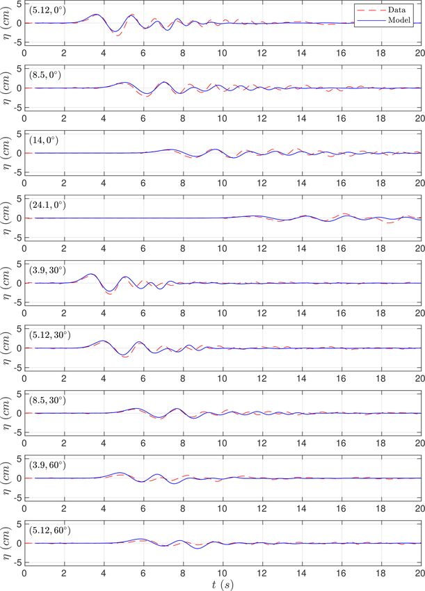
We would like to stress the simplicity of the slide model Figure 3 depicts the modeled times series for the water height
used here as a great advantage regarding parameter setup. at the four wave gages and compares them with the lab-
Although the end user has to adjust some input parameters measured data. Note that the computed free surface matches
of the model, within a range of acceptable value, the sim- well with the laboratory data for gauges WG2–WG4, both in
plicity of the proposed numerical model makes this task re- amplitude and frequency. For gauge WG1, some mismatch is
main simple – not representing an obstacle to run the model. observed in amplitude, which could be explained by the sim-
On the other hand, the efficient GPU implementation of the plicity of the landslide model and the absence of turbulent
model allows for performing uncertainty quantification (see effects in the model.
Sánchez-Linares et al., 2016) on a few parameters and inves- Figure 4 shows the location and evolution of the granular
tigating the sensitivity to them, varying on small ranges (as material and water free surface at several times during the
in González-Vida et al., 2019). This will be the aim of future numerical simulation. In Grilli et al. (2017) some snapshots
works. When field or experimental observations are avail- of the landslide evolution are shown at different time steps.
able, a different approach is proposed in Ferreiro-Ferreiro Compared to those snapshots, it can be observed that the lo-
et al. (2020), where an automatic data assimilation strategy cation of the landslide front is well captured by the model,
for a similar landslide non-hydrostatic model is proposed. but there is some mismatch in the landslide shape at the front,
The same strategy can be adapted for the model used here. mainly due to the simplicity of the landslide model consid-
ered here. In particular, we consider that density remains con-
5.1 Benchmark problem 4: two-dimensional stant in the landslide layer during the simulation, which is not
submarine granular slide true due to the water entrainment.
In the numerical experiments presented in this section, the
The first proposed benchmark problem for granular slides,
number of layers was set up to five. Similar results were
BP4 in the list, aims to reproduce the generation of tsunamis
obtained with a lower number of layers (four or three) but
by submarine granular slides modeled in the laboratory
slightly closer to measured data when considering five layers.
experiment by means of glass beads. The corresponding
This justifies our choice in the present test problem. A larger
2D laboratory experiments were performed at the École Cen-
number of layers does not further improve the numerical re-
trale de Marseille (see Grilli et al., 2017, for a description of
sults. This may indicate that to get better numerical results,
the experiment). A set of 58 (29 with their corresponding
it is no longer a question related to the dispersive properties
replicate) experiments were performed at the IRPHE (Insti-
of the model (which improve with the number of layers) but
tut de Recherche sur les Phénomènes Hors Equilibre) pre-
is more likely due to some missing physics.
cision tank. The experiments were performed using a trian-
gular submarine cavity filled with glass beads that were re-
leased by lifting a sluice gate and then moving down a plane
slope, all underwater. Figure 2 shows a schematic picture of
the experiment setup.
https://doi.org/10.5194/nhess-21-791-2021 Nat. Hazards Earth Syst. Sci., 21, 791–805, 2021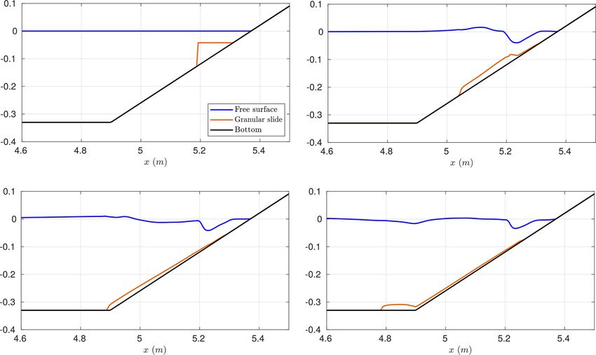
798                        J. Macías et al.: Multilayer-HySEA model validation for landslide-generated tsunamis – Part 2

                                                                    14.8 cm, and L = 11 cm. Case 2 is given by ds = 10 mm,
                                                                    H = 15 cm, and L = 13.5 cm. The benchmark problem pro-
                                                                    posed consists of simulating the free-surface elevation evolu-
                                                                    tion at the four gauges WG1 to WG4, where measured data
                                                                    are provided, for the two test cases described above.
                                                                       The same model configuration as in the previous bench-
                                                                    mark problem is used here. The vertical structure is re-
                                                                    produced using three layers in the present case. The one-
                                                                    dimensional domain is given by the interval [0, 2.2], and it is
                                                                    discretized using a step 1x = 0.003 m. As boundary condi-
                                                                    tions, rigid walls were imposed. The simulation time is 2.5 s.
                                                                    The CFL number is set to 0.9, and the model parameters take
                                                                    the following values:

                                                                    g = 9.81, r = 0.6, na = 10−2 , nm = 9 × 10⁻² ,
                                                                    δ1 = 6◦ , δ2 = 26◦ , δ3 = 12◦ , β = 0.136, γ = 10−3 .

                                                                    Finally ds was set to 1.5 × 10⁻³ and 10 × 10−3 depending on
                                                                    the test case.
                                                                       Figure 6 shows the comparison for Case 1. In this case, the
                                                                    numerical results show a very good agreement when com-
                                                                    pared with lab-measured data, and, in particular, the two
                                                                    leading waves are very well captured. Figure 7 shows the
                                                                    comparison for Case 2. In this case, the agreement is good,
Figure 3. Numerical time series for the simulated water surface
                                                                    but larger differences between model and lab measurements
(in blue) compared with lab-measured data (red) at wave gauges
(a) WG1, (b) WG2, (c) WG3, and (d) WG4.                             can be observed.
                                                                       Two things can be concluded from the observation of
                                                                    Figs. 6 and 7: (1) a much better agreement is obtained for
                                                                    Case 1 than for Case 2 and (2) the agreement is better for
5.2   Benchmark problem 5: two-dimensional subaerial                gauges located farther from the slide compared with closer
      granular slide                                                to the slide gauges. Although paradoxical, this second dif-
                                                                    ferential behavior among gauges can be explained as a con-
This benchmark is based on a series of 2D laboratory exper-         sequence of the hydrodynamic component being much bet-
iments performed by Viroulet et al. (2014) in a small tank at       ter resolved and simulated than the morphodynamic compo-
the École Centrale de Marseille, France. The simplified pic-        nent (the movement of the slide material), which is obviously
ture of the setup for these experiments can be found in Fig. 5.     much more difficult to reproduce. But, at the same time, this
   The granular material was confined in triangular subaerial       implies a correct transfer of energy at the initial stages of the
cavities and composed of dry glass beads of diameter ds             interaction between the slide and fluid.
(which was varied) and density ρs = 2500 km m−3 . This was             Finally, Fig. 8 shows the location of the granular material
located on a plane with a 45◦ slope just on top of the water        and the free-surface elevation at several times for the numeri-
surface. Then the slide was released by lifting a sluice gate       cal simulation of Case 1. In Viroulet et al. (2014) some snap-
and coming in contact with water right away. The experimen-         shots of the landslide evolution are shown at different time
tal setup used by Viroulet et al. (2014) consisted of a wave        steps that can be compared with Fig. 8. As for the bench-
tank 2.2 m long, 0.4 m high, and 0.2 m wide.                        mark problem 4, it can be seen that the location of the land-
   The granular material is initially retained by a vertical gate   slide front is well captured, but there is some mismatch in the
on the dry slope. The gate is suddenly lowered, and in the          landslide shape at the front, mainly due to the simplicity of
numerical experiments, it should be assumed that the gate re-       the landslide model considered here.
lease velocity is large enough to neglect the time it takes the
gate to withdraw. The front face of the granular slide touches      5.3   Benchmark problem 6: three-dimensional
the water surface at t = 0. The initial slide shape has a tri-            subaerial granular slide
angular cross section over the width of the tank, with down-
tank length L and front face height B = L as the slope angle        This benchmark problem is based on the 3D laboratory ex-
is 45◦ .                                                            periment of Mohammed and Fritz (2012) and Mohammed
   For the present benchmark, two cases are considered.             (2010). Benchmark 6 simulates the rapid entry of a granu-
Case 1 is defined by the following setup: ds = 1.5 mm, H =          lar slide into a 3D water body. The landslide tsunami exper-

Nat. Hazards Earth Syst. Sci., 21, 791–805, 2021                                     https://doi.org/10.5194/nhess-21-791-2021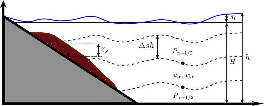
J. Macías et al.: Multilayer-HySEA model validation for landslide-generated tsunamis – Part 2                                         799

Figure 4. Modeled location of the granular material and water free surface elevation at times t = 0, 0.3, 0.6, and 0.9 s.

Figure 5. BP5 sketch of the setup for the laboratory experiments.

iments were conducted at Oregon State University in Cor-
vallis. The landslides are deployed off a plane with a 27.1◦
slope, as shown in Fig. 9.
   The landslide material is deployed using a box measur-
ing 2.1 m × 1.2 m × 0.3 m, with a volume of 0.756 m3 , and
weighting approximately 1360 kg. The case selected by the
NTHMP as a benchmarking test is the one with a still-water
depth of H = 0.6 m (see Fig. 9). The computational domain
is the rectangle defined by [0, 48] × [−14, 14], and it is dis-
cretized with 1x = 1y = 0.06 m. At the boundaries, wall
boundary conditions were imposed. The simulation time is
20 s and we set the CFL = 0.5. According to Mohammed and
Fritz (2012) and Mohammed (2010), the three-dimensional
granular landslide parameters were set to

g = 9.81, r = 0.55, na = 4, nm = 4 × 10⁻² ,
                                                                          Figure 6. Numerical time series for the simulated water surface
ds = 13.7 × 10⁻³ , δ1 = 6◦ , δ2 = 30◦ , δ3 = 12◦ ,                        (in blue) compared with lab-measured data (red). Case 1 at gauges
β = 0.136, γ = 10−3 .                                                     (a) G1, (b) G2, (c) G3, and (d) G4.

https://doi.org/10.5194/nhess-21-791-2021                                            Nat. Hazards Earth Syst. Sci., 21, 791–805, 2021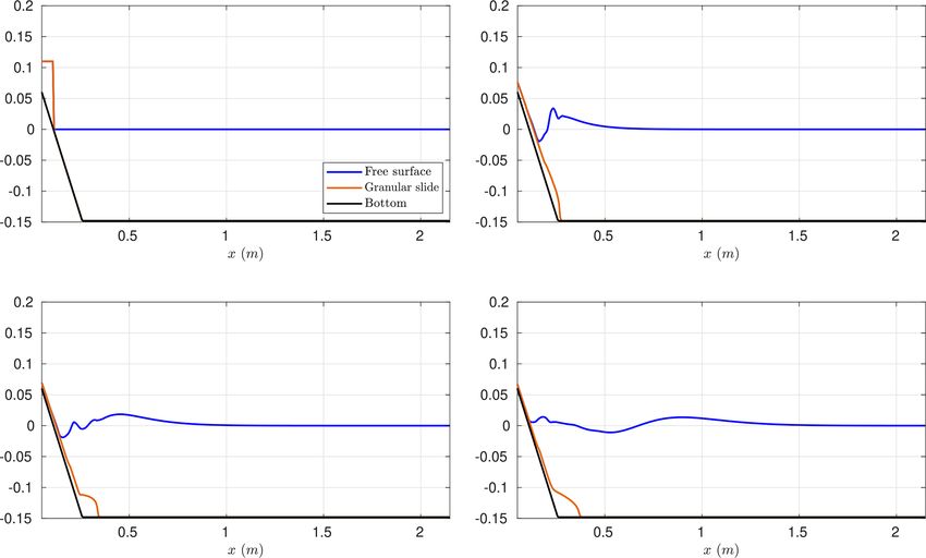
800                           J. Macías et al.: Multilayer-HySEA model validation for landslide-generated tsunamis – Part 2

                                                                    Table 1. Location of the nine waves gauges referenced to the toe’s
                                                                    slope.

                                                                     θ◦                 0◦                        30◦                  60◦
                                                                     R     5.12   8.5        14   24.1    3.9     5.12     8.5   3.9     5.12

                                                                    Table 2. Wall-clock times in seconds for the hydrostatic shallow-
                                                                    water Savage–Hutter system (SWE-SH) and the non-hydrostatic
                                                                    GPU implementations. The ratios are with respect to the SWE-SH
                                                                    model implementation.

                                                                                                     Runtime (s)         Ratio
                                                                                   SWE-SH                186.55             1
                                                                                   1L NH-SH              541.11           2.9
                                                                                   2L NH-SH              649.19          3.48
                                                                                   3L NH-SH              869.32          4.66

                                                                    The slide impact velocity measured in the lab experiment
                                                                    is 5.72 m s−1 at time t = 0.44 s. The numerically computed
                                                                    slide impact velocity is slightly underestimated with a value
                                                                    of 5.365 m s−1 at time t = 0.4 s as it can be seen in the up-
Figure 7. Numerical time series for the simulated water surface     per panel of Fig. 10. The final simulated granular deposit is
(in blue) compared with lab-measured data (red). Case 2 at gauges   located partially on the final part of the sloping floor and par-
(a) G1, (b) G2, (c) G3, and (d) G4.                                 tially at the flat bottom closer to the point of change of slope
                                                                    as is shown in the lower panel of Fig. 10. This can be com-
                                                                    pared with the actual final location of the granular material
The vertical structure of the fluid layer is modeled using three    in the experimental setup. The simulated deposits, being thin-
layers. Similar results were obtained with two layers.              ner, extend further. This is probably due to the fact that we
   Initially, the slide box is driven using four pneumatic          are neglecting the friction that it is produced by the change in
pistons. Here we provide comparisons for the case where             the slope at the transition area. In Ma et al. (2015) a similar
the pressure for the pneumatic pistons generating the slide         result and discussion can be found.
is P = 0.4 MPa (P = 58 PSI). In Mohammed (2010), it is                 Figure 11 presents the comparisons between the simulated
shown that for this test
                       √ case, the landslide box reached a          and the measured waves at the nine gauges we have retained.
velocity of vb = 2.3 · g · 0.6 = 5.58 m s−1 . Thus, the initial     Model results are in good agreement with measured time.
condition for the water velocities is set to zero,                  Despite this, wave heights are overestimated at some stations,
ui = 0, i = 1, 2, . . ., L,                                         specially those closer to the shoreline (for example, the sta-
                                                                    tion with R = 3.9 and θ = 30◦ ). This effect has been also ob-
and for the landslide velocity it is set to the above-mentioned     served and discussed in Ma et al. (2015). At some of the time
constant value,                                                     series, it can be observed that the small free-surface oscilla-
us = 5.58, wherever zs > 0,                                         tions at the final part of the time series are not well captured
                                                                    by the model. This is partially due to the relatively coarse
for the x component. The y component of the landslide ve-           horizontal grids used in the simulation. This same behavior
locity was initially set to zero.                                   can be also observed in Fig. 12 in this case for the com-
   The benchmark problem proposed consists of simulating            parisons between the simulated and measured run-up values
the free-surface elevation at some wave gauges. In the present      at some measure locations situated at the shoreline (as for
study, we include the comparison for the nine wave gauges           x = 7.53).
displayed in Fig. 9 as red dots. A total number of 21 wave             Table 2 shows the wall-clock times on an NVIDIA
gauges composed the whole set of data plus five run-up              Tesla P100 GPU. It can be observed that including non-
gauges. The wave gauges in coordinates (R, θ ◦ ) are given          hydrostatic terms in the SWE-SH system results in an in-
more precisely in Table 1.                                          crease in the computational time of 2.9 times. If a richer ver-
   Before comparing time series, we first check the simu-           tical structure is considered, then larger computational times
lated landslide velocity at impact with the measured one.           are required. As in the examples for the two- and three-layer

Nat. Hazards Earth Syst. Sci., 21, 791–805, 2021                                        https://doi.org/10.5194/nhess-21-791-2021
J. Macías et al.: Multilayer-HySEA model validation for landslide-generated tsunamis – Part 2 801
Figure 8. Modeled water free-surface elevation and granular slide location at times t = 0, 0.2, 0.4, and 0.8 s for Case 1.
systems, there is a 3.48 and 4.66 times increase in the com-
putational effort.
6 Concluding remarks
Numerical models need to be validated prior to their use as
predictive tools. This requirement becomes even more neces-
sary when these models are going to be used for risk assess-
ment in natural hazards where human lives are involved. The
current work aims at benchmarking the novel Multilayer-
HySEA model for landslide-generated tsunamis produced by
granular slides, in order to provide the tsunami community
with a robust, efficient, and reliable tool for landslide tsunami
hazard assessment in the future.
The Multilayer-HySEA code implements a two-phase
model to describe the interaction between landslides (aerial
or subaerial) and water body. The upper phase describes the
hydrodynamic component. This is done using a stratified ver-
tical structure that includes non-hydrostatic terms in order
to include dispersive effects in the propagation of simulated
waves. The motion of the landslide is taken into account by
the lower phase, consisting of a Savage–Hutter model. To re-
produce these flows, the friction model given in Pouliquen
Figure 9. Schematic picture of the computational domain. Plan and Forterre (2002) is considered here. The hydrodynamic
view in panel (a). Cross section at y = 0 m in panel (b). The red and morphodynamic models are weakly coupled through the
dots represent the distribution of the wave gauge positions in the boundary condition at their interface.
laboratory setup. The implemented numerical algorithm combines a finite-
volume path-conservative scheme for the underlying hyper-
bolic system and finite differences for the discretization of
the non-hydrostatic terms. The numerical model is imple-
https://doi.org/10.5194/nhess-21-791-2021 Nat. Hazards Earth Syst. Sci., 21, 791–805, 2021802 J. Macías et al.: Multilayer-HySEA model validation for landslide-generated tsunamis – Part 2 Figure 10. BP6 cross section at y = 0 m. Panel (a) shows the location and velocity of the granular slide and the generated wave at time t = 0.4 s from the triggering and (b) the final deposit location (at t = 20 s). Figure 11. Simulated (solid blue lines) time series compared with measured (dashed red lines) free-surface waves for the nine wave gauges considered at (R, θ ◦ ) positions. Nat. Hazards Earth Syst. Sci., 21, 791–805, 2021 https://doi.org/10.5194/nhess-21-791-2021
J. Macías et al.: Multilayer-HySEA model validation for landslide-generated tsunamis – Part 2                                         803

Figure 12. Time series comparing numerical run-up (solid blue) at the four run-up gauges with the measured (dashed red) data at (x, y) po-
sitions.

mented to be run in GPU architectures. The two-layer non-              Data availability. All the data used in the present work and nec-
hydrostatic code coupled with the Savage–Hutter used here              essary to reproduce the setup of the numerical experiments as
has been shown to run at very efficient computational times.           well as the laboratory-measured data to compare with can be
To assess this, we compare with respect to the one-layer               downloaded from LTMBW (2017) at http://www1.udel.edu/kirby/
SWE/Savage–Hutter GPU code. For the numerical simu-                    landslide/ (last access: 21 February 2021).
lations performed here, the execution times for the non-
hydrostatic model are always below 4.66 times the times for
                                                                       Author contributions. JM led the HySEA codes benchmarking ef-
the SWE model for a number of layers up to three. We can
                                                                       fort undertaken by the EDANYA group, wrote most of the paper, re-
conclude that the numerical scheme presented here is very
                                                                       viewed and edited it, and assisted in the numerical experiments and
robust, is extremely efficient, and can model dispersive ef-           in their setup. CE implemented the numerical code and performed
fects generated by submarine/subaerial landslides at a low             all the numerical experiments; he also contributed to the writing of
computational cost considering that dispersive effects and a           the manuscript. JM and CE did all the figures. MC significantly con-
vertical multilayer structure are included in the model. Model         tributed to the design and implementation of the numerical code.
results show a good agreement with the experimental data for
the three benchmark problems considered, in particular for
BP5, but this also occurs for the other two benchmark prob-            Competing interests. The authors declare that they have no conflict
lems. In general, a better agreement for the hydrodynamic              of interest.
component, compared with its morphodynamic counterpart,
is shown, which is more challenging to reproduce.
                                                                       Acknowledgements. The authors are indebted to Diego Arcas
                                                                       (PMEL/NOAA) and Victor Huérfano (PRSN) for supporting our
Code availability. The numerical code is currently under develop-      participation in the 2017 Galveston workshop and to the MMS of
ment and only available to close collaborators. In the future, we      the NTHMP for kindly inviting us to that event.
will provide an open version of the code as we already do for
Tsunami-HySEA. This version will be available from the web-
site https://edanya.uma.es/hysea/ (last access: 21 February 2021)      Financial support. This research has been supported by the
(Macías, 2021). Finally, the NetCDF files containing the numer-        Spanish Government–FEDER (project MEGAFLOW) (grant
ical results obtained with the Multilayer-HySEA code for all the       no. RTI2018-096064-B-C21) and the Junta de Andalucía–FEDER
tests presented here can be found and download from Macías et al.      (grant no. UMA18-Federja-161).
(2020b).

https://doi.org/10.5194/nhess-21-791-2021                                        Nat. Hazards Earth Syst. Sci., 21, 791–805, 2021
804 J. Macías et al.: Multilayer-HySEA model validation for landslide-generated tsunamis – Part 2
Review statement. This paper was edited by Maria Ana Baptista Fine, I. V., Rabinovich, A. B., and Kulikov, E. A.: Numerical mod-
and reviewed by two anonymous referees. elling of landslide generated tsunamis with application to the
Skagway Harbor tsunami of November 3, 1994, in: Proc. Intl.
Conf. on Tsunamis, Paris, 211–223, 1998.
Fritz, H. M., Hager, W. H., and Minor, H.-E.: Near field
References characteristics of landslide generated impulse waves,
J. Waterway Port Coast. Ocean Eng., 130, 287–302,
Abadie, S., Morichon, D., Grilli, S., and Glockner, S.: Nu- https://doi.org/10.1061/(ASCE)0733-950X(2004)130:6(287),
merical simulation of waves generated by landslides using a 2004.
multiple-fluid Navier–Stokes model, Coast. Eng., 57, 779–794, Garres-Díaz, J., Fernández-Nieto, E. D., Mangeney, A.,
https://doi.org/j.coastaleng.2010.03.003, 2010. and de Luna, T. M.: A weakly non-hydrostatic shal-
Abadie, S. M., Harris, J. C., Grilli, S. T., and Fabre, R.: Numerical low model for dry granular flows, J. Scient. Comput., 86,
modeling of tsunami waves generated by the flank collapse of https://doi.org/10.1007/s10915-020-01377-9, 2021.
the Cumbre Vieja Volcano (La Palma, Canary Islands): Tsunami González-Vida, J., Macías, J., Castro, M., Sánchez-Linares,
source and near field effects, J. Geophys. Res.-Oceans, 117, C., Ortega, S., and Arcas, D.: The Lituya Bay landslide-
C05030, https://doi.org/10.1029/2011JC007646, 2012. generated mega-tsunami. Numerical simulation and sensitiv-
Adsuara, J., Cordero-Carrión, I., Cerdá-Durán, P., and ity analysis, Nat. Hazards Earth Syst. Sci., 19, 369–388,
Aloy, M.: Scheduled relaxation Jacobi method: Improve- https://doi.org/10.5194/nhess-19-369-2019, 2019.
ments and applications, J. Comput. Phys., 321, 369–413, Grilli, S. T., Shelby, M., Kimmoun, O., Dupont, G., Nicolsky, D.,
https://doi.org/10.1016/j.jcp.2016.05.053, 2016. Ma, G., Kirby, J. T., and Shi, F.: Modeling coastal tsunami haz-
Ataie-Ashtiani, B. and Najafi-Jilani, A.: Laboratory investigations ard from submarine mass failures: effect of slide rheology, ex-
on impulsive waves caused by underwater landslide, Coast. Eng., perimental validation, and case studies off the US East Coast,
55, 989–1004, https://doi.org/10.1016/j.coastaleng.2008.03.003, Nat. Hazards, 86, 353–391, https://doi.org/10.1007/s11069-016-
2008. 2692-3, 2017.
Ataie-Ashtiani, B. and Shobeyri, G.: Numerical simulation of Harbitz, C. B., Pedersen, G., and Gjevik, B.: Numerical sim-
landslide impulsive waves by incompressible smoothed parti- ulations of large water waves due to landslides, J. Hydraul.
cle hydrodynamics, Int. J. Numer. Meth. Fluids, 56, 209–232, Eng., 119, 1325–1342, https://doi.org/10.1061/(ASCE)0733-
https://doi.org/10.1002/fld.1526, 2008. 9429(1993)119:12(1325), 1993.
Brunet, M., Moretti, L., Le Friant, A., Mangeney, A., Fernández Ni- Heinrich, P.: Nonlinear water waves generated by subma-
eto, E. D., and Bouchut, F.: Numerical simulation of the 30– rine and aerial landslides, J. Waterway Port Coast. Ocean
45 ka debris avalanche flow of Montagne Pelée volcano, Mar- Eng., 118, 249–266, https://doi.org/10.1061/(ASCE)0733-
tinique: from volcano flank collapse to submarine emplacement, 950X(1992)118:3(249), 1992.
Nat. Hazards, 87, 1189–1222, 2017. Heller, V. and Hager, W.: Impulse product parameter in land-
Castro, M. and Fernández-Nieto, E.: A class of computationally fast slide generated impulse waves, J. Waterway Port Coast. Ocean
first order finite volume solvers: PVM methods, SIAM J. Scient. Eng., 136, 145–155, https://doi.org/10.1061/(ASCE)WW.1943-
Comput., 34, A2173–A2196, 2012. 5460.0000037, 2010.
Castro, M., Ortega, S., de la Asunción, M., Mantas, J., and Gallardo, Horrillo, J., Wood, A., Kim, G.-B., and Parambath, A.: A simplified
J.: GPU computing for shallow water flow simulation based on 3-D Navier–Stokes numerical model for landslide-tsunami: Ap-
finite volume schemes, Comptes Rendus Mécanique, 339, 165– plication to the Gulf of Mexico, J. Geophys. Res.-Oceans, 118,
184, 2011. 6934–6950, https://doi.org/10.1002/2012JC008689, 2013.
Escalante, C., Fernández-Nieto, E., Morales, T., and Castro, Kirby, J. T., Shi, F., Nicolsky, D., and Misra, S.: The 27 April 1975
M.: An efficient two–layer non-hydrostatic approach for Kitimat, British Columbia, submarine landslide tsunami: a com-
dispersive water waves, J. Scient. Comput., 79, 273–320, parison of modeling approaches, Landslides, 13, 1421–1434,
https://doi.org/10.1007/s10915-018-0849-9, 2018a. https://doi.org/10.1007/s10346-016-0682-x, 2016.
Escalante, C., Morales, T., and Castro, M.: Non-hydrostatic pres- Kirby, J. T., Grilli, S. T., Zhang, C., Horrillo, J., Nicolsky, D.,
sure shallow flows: GPU implementation using finite volume and and Liu, P. L.-F.: The NTHMP Landslide Tsunami Benchmark
finite difference scheme, Appl. Math. Comput., 338, 631–659, Workshop, Galveston, January 9–11, 2017, Tech. rep., Re-
https://doi.org/10.1016/j.amc.2018.06.035, 2018b. search Report CACR-18-01, available at: http://www1.udel.edu/
Fernández-Nieto, E., Bouchut, F., Bresch, D., Castro, M., and kirby/landslide/report/kirby-etal-cacr-18-01.pdf (last access:
Mangeney, A.: A new Savage-Hutter type model for submarine 20 February 2021), 2018.
avalanches and generated tsunami, J. Comput. Phys., 227, 7720– LTMBW: Landslide Tsunami Model Benchmarking Workshop,
7754, 2008. Galveston, Texas, 2017, available at: http://www1.udel.edu/
Fernández-Nieto, E., Parisot, M., Penel, Y., and Sainte-Marie, J.: A kirby/landslide/index.html (last access: 21 April 2020), 2017.
hierarchy of dispersive layer-averaged approximations of Euler Ma, G., Shi, F., and Kirby, J. T.: Shock-capturing
equations for free surface flows, Commun. Math. Sci., 16, 1169– non-hydrostatic model for fully dispersive sur-
1202, 2018. face wave processes, Ocean Model., 43–44, 22–35,
Ferreiro-Ferreiro, A., García-Rodríguez, J., López-Salas, J., Es- https://doi.org/10.1016/j.ocemod.2011.12.002, 2012.
calante, C., and Castro, M.: Global optimization for data as- Ma, G., Kirby, J. T., and Shi, F.: Numerical simu-
similation in landslide tsunami models, J. Comput. Phys., 403, lation of tsunami waves generated by deformable
109069, https://doi.org/10.1016/j.jcp.2019.109069, 2020.
Nat. Hazards Earth Syst. Sci., 21, 791–805, 2021 https://doi.org/10.5194/nhess-21-791-2021J. Macías et al.: Multilayer-HySEA model validation for landslide-generated tsunamis – Part 2 805
submarine landslides, Ocean Model., 69, 146–165, Mangeney, A., Bouchut, F., Thomas, N., Vilotte, J. P., and Bristeau,
https://doi.org/10.1016/j.ocemod.2013.07.001, 2013. M. O.: Numerical modeling of self-channeling granular flows
Ma, G., Kirby, J. T., Hsu, T.-J., and Shi, F.: A two- and of their levee-channel deposits, J. Geophys. Res.-Earth, 112,
layer granular landslide model for tsunami wave genera- F02017, https://doi.org/10.1029/2006JF000469, 2007.
tion: Theory and computation, Ocean Model., 93, 40–55, Mohammed, F.: Physical modeling of tsunamis generated by three-
https://doi.org/10.1016/j.ocemod.2015.07.012, 2015. dimensional deformable granular landslides, PhD thesis, Georgia
Macías, J.: HySEA codes web page, available at: https://edanya. Institute of Technology, Atlanta, GA, USA, 2010.
uma.es/hysea/, last access: 21 February 2021. Mohammed, F. and Fritz, H. M.: Physical modeling of
Macías, J., Vázquez, J., Fernández-Salas, L., González-Vida, tsunamis generated by three-dimensional deformable gran-
J., Bárcenas, P., Castro, M., del Río, V. D., and Alonso, ular landslides, J. Geophys. Res.-Oceans, 117, C11015,
B.: The Al-Borani submarine landslide and associated https://doi.org/10.1029/2011JC007850, 2012.
tsunami. A modelling approach, Mar. Geol., 361, 79–95, Pouliquen, O. and Forterre, Y.: Friction law for dense gran-
https://doi.org/10.1016/j.margeo.2014.12.006, 2015. ular flows: application to the motion of a mass down
Macías, J., Castro, M., Ortega, S., Escalante, C., and González- a rough inclined plane, J. Fluid Mech., 453, 133–151,
Vida, J.: Performance Benchmarking of Tsunami-HySEA Model https://doi.org/10.1017/S0022112001006796, 2002.
for NTHMP’s Inundation Mapping Activities, Pure Appl. Rzadkiewicz, S. A., Mariotti, C., and Heinrich, P.: Numerical
Geophys., 174, 3147–3183, https://doi.org/10.1007/s00024-017- simulation of submarine landslides and their hydraulic ef-
1583-1, 2017. fects, J. Waterway Port Coast. Ocean Eng., 123, 149–157,
Macías, J., Escalante, C., Castro, M., González-Vida, J., and https://doi.org/10.1061/(ASCE)0733-950X(1997)123:4(149),
Ortega, S.: HySEA model, Landslide Benchmarking Results, 1997.
NTHMP report, Tech. rep., Universidad de Málaga, Málaga, Sánchez-Linares, C., de la Asunción, M., Castro, M., Vida, J. G.,
https://doi.org/10.13140/RG.2.2.27081.60002, 2017. Macías, J., and Mishra, S.: Uncertainty quantification in tsunami
Macías, J., Escalante, C., and Castro, M.: Performance assess- modeling using multi-level Monte Carlo finite volume method,
ment of Tsunami-HySEA model for NTHMP tsunami cur- J. Math. Indust., 6, 5, https://doi.org/10.1186/s13362-016-0022-
rents benchmarking. Laboratory data, Coast. Eng., 158, 103667, 8, 2016.
https://doi.org/10.1016/j.coastaleng.2020.103667, 2020a. Savage, S. and Hutter, K.: The motion of a finite mass of granular
Macías, J., Escalante, C., and Castro, M.: Numerical results material down a rough incline, J. Fluid Mech., 199, 177–215,
in Multilayer-HySEA model validation for landslide gener- https://doi.org/10.1017/S0022112089000340, 1989.
ated tsunamis. Part II Granular slides, Dataset on Mendeley, Viroulet, S., Sauret, A., and Kimmoun, O.: Tsunami generated
https://doi.org/10.17632/94txtn9rvw.2, 2020b. by a granular collapse down a rough inclined plane, Europhys.
Macías, J., Ortega, S., González-Vida, J., and Castro, M.: Per- Lett., 105, 34004, https://doi.org/10.1209/0295-5075/105/34004,
formance assessment of Tsunami-HySEA model for NTHMP 2014.
tsunami currents benchmarking. Field cases, Ocean Model., 152, Weiss, R., Fritz, H. M., and Wünnemann, K.: Hybrid mod-
101645, https://doi.org/10.1016/j.ocemod.2020.101645, 2020c. eling of the mega-tsunami runup in Lituya Bay af-
Macías, J., Escalante, C., and Castro, M. J.: Multilayer-HySEA ter half a century, Geophys. Res. Lett., 36, L09602,
model validation for landslide-generated tsunamis – Part 1: https://doi.org/10.1029/2009GL037814, 2009.
Rigid slides, Nat. Hazards Earth Syst. Sci., 21, 775–789, Yavari-Ramshe, S. and Ataie-Ashtiani, B.: Numerical modeling
https://doi.org/10.5194/nhess-21-775-2021, 2021. of subaerial and submarine landslide-generated tsunami waves–
recent advances and future challenges, Landslides, 13, 1325–
1368, https://doi.org/10.1007/s10346-016-0734-2, 2016.
https://doi.org/10.5194/nhess-21-791-2021 Nat. Hazards Earth Syst. Sci., 21, 791–805, 2021You can also read