Retrieval algorithm for the column CO2 mixing ratio from pulsed multi-wavelength lidar measurements
←
→
Page content transcription
If your browser does not render page correctly, please read the page content below
Atmos. Meas. Tech., 14, 3909–3922, 2021
https://doi.org/10.5194/amt-14-3909-2021
© Author(s) 2021. This work is distributed under
the Creative Commons Attribution 4.0 License.

Retrieval algorithm for the column CO2 mixing ratio from pulsed
multi-wavelength lidar measurements
Xiaoli Sun1 , James B. Abshire1,2 , Anand Ramanathan1,a , Stephan R. Kawa1 , and Jianping Mao1,2
1 NASA   Goddard Space Flight Center, Science and Exploration Directorate, Greenbelt, Maryland, USA
2 Universityof Maryland, College Park, Maryland, USA
a now at: Audible, Inc., Newark, New Jersey, USA

Correspondence: Xiaoli Sun (xiaoli.sun-1@nasa.gov)

Received: 26 November 2020 – Discussion started: 22 December 2020
Revised: 17 March 2021 – Accepted: 9 April 2021 – Published: 27 May 2021

Abstract. The retrieval algorithm for CO2 column mixing            1   Introduction
ratio from measurements of a pulsed multi-wavelength inte-
grated path differential absorption (IPDA) lidar is described.
The lidar samples the shape of the 1572.33 nm CO2 absorp-          Accurate remote sensing of atmospheric CO2 from Earth-
tion line at multiple wavelengths. The algorithm uses a least-     orbiting satellites is a key component in a long-term carbon–
squares fit between the CO2 line shape computed from a             climate observing system (Sellers et al., 2018). Airborne and
layered atmosphere model and that sampled by the lidar.            spaceborne lidar can be used to remotely monitor the global
In addition to the column-average CO2 dry-air mole frac-           CO2 and other trace-gas concentrations under conditions that
tion (XCO2 ), several other parameters are also solved si-         are inaccessible to passive spaceborne CO2 measurement
multaneously from the fit. These include the Doppler shift         missions, such as GOSAT (Kuze et al., 2016), OCO-2 (Crisp
at the received laser signal wavelength, the product of the        et al., 2017), and OCO-3 (Eldering et al., 2017, 2019). Stud-
surface reflectivity and atmospheric transmission, and a lin-      ies have shown (Kawa et al., 2018) that a polar-orbiting inte-
ear trend in the lidar receiver’s spectral response. The algo-     grated path differential absorption (IPDA) lidar can measure
rithm can also be used to solve for the average water vapor        XCO2 with low bias and high precision at all sun angles,
mixing ratio, which produces a secondary absorption in the         seasons, and latitudes using a constant nadir-zenith illumi-
wings of the CO2 absorption line under humid conditions.           nation and observation geometry. A pulsed IPDA lidar also
The least-squares fit is linearized about the expected XCO2        provides the range-resolved atmospheric backscatter profiles,
value, which allows the use of a standard linear least-squares     so that return signals from the surface, clouds, and aerosols
fitting method and software tools. The standard deviation of       can be uniquely separated (Allan et al., 2019). This allows
the retrieved XCO2 is obtained from the covariance matrix of       pulsed IPDA lidar to measure XCO2 to the surface, cloud
the fit. The averaging kernel is also provided similarly to that   tops, or both (Ramanathan et al., 2015). Because the laser
used for passive trace-gas column measurements. Examples           pulses reflected from clouds, aerosols, and surface are sepa-
are presented of using the algorithm to retrieve XCO2 from         rated in time, the XCO2 retrievals to the ground surface are
measurements of the NASA Goddard airborne CO2 Sounder              not biased by scattering from clouds and aerosols (Mao et al.,
lidar that were made at constant altitude and during spiral-       2018).
down profile maneuvers.                                               Several types of dual-wavelength (online and offline)
                                                                   IPDA lidar have been demonstrated previously for measur-
                                                                   ing XCO2 from aircraft (Spiers et al., 2011; Menzies et al.,
                                                                   2014; Jacob et al., 2019; Dobler et al., 2013; Campbell et
                                                                   al., 2020; Refaat et al., 2016, 2020, 2021; Amediek et al.,
                                                                   2017; Zhu et al., 2019, 2020). A multi-wavelength IPDA li-
                                                                   dar has also been reported. The retrieval algorithms used in

Published by Copernicus Publications on behalf of the European Geosciences Union.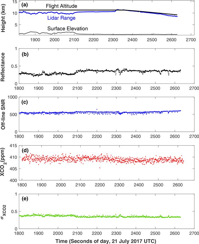
3910 X. Sun et al.: Retrieval algorithm for XCO2 from lidar measurements
these IPDA lidars calculate the ratios of online to offline at- consists of a tunable seed laser, a pulsed modulator, and
mosphere transmission, convert them to differential absorp- a power amplifier. The seed laser module consists of two
tion optical depths (DAODs), and then solve for XCO2 from single-frequency continuous-wave (CW) diode lasers. One is
the DAOD based on atmospheric transmission models. For the reference laser whose wavelength is locked to the cen-
the multi-wavelength lidar proposed by Han et al. (2020), ter of the CO2 absorption line in a gas cell. The other diode
a series of DAODs are calculated, and a least-squares fit is laser (slave) is tunable and its wavelength is locked to that of
used to solve for XCO2 (Han et al., 2020). The XCO2 can be the master, plus a programmable offset frequency. The off-
solved directly from the DAOD; however, these algorithms set frequency is step-tuned across the CO2 absorption line.
rely on the accurate knowledge of the line shape of the CO2 The number of laser wavelengths in the scan and the exact
absorption. They are sensitive to measurement biases due to wavelength of each laser pulse are digitally pre-programmed
uncertainties in spectroscopy and meteorological conditions and can be adjusted via software commands (Numata et al.,
that affect the line shape. They also require precise knowl- 2012). An electro-optical modulator is used to gate the out-
edge of the laser wavelengths, the lidar receiver optical trans- put of the slave laser into 1 µs wide pulses. The laser pulses
mission versus wavelength, and the Doppler shift of the re- are then amplified by a multi-stage commercial fiber laser
ceived laser signals. amplifier. The airborne lidar’s laser pulse rate is 10 kHz and
NASA Goddard Space Flight Center (GSFC) has devel- there are 30 wavelengths per scan, which gives a wavelength
oped an airborne multi-wavelength CO2 sounder lidar and scan rate of about 300 Hz. The transmitted laser pulse energy
demonstrated XCO2 measurements through a series of air- at each wavelength is also sampled, and the results are used
borne campaigns (Abshire et al., 2010, 2013, 2014, 2018; to normalize the received signal to correct for fluctuations in
Ramanathan et al., 2013, 2015, 2018; Mao et al., 2018). the transmitted laser energy with wavelength.
Its retrieval compares the lidar-sampled line shape with one The lidar receiver detects and records the received laser
computed from an atmosphere model to retrieve XCO2 . Sev- pulse waveform over the entire atmosphere column traveled
eral other parameters, such as the Doppler shift, surface by the laser pulses. In the airborne lidar all signals are dig-
reflectance, and lidar receiver spectral response are solved itized and recorded and the lidar analysis is performed on
simultaneously via a least-squares fit. The retrieval algo- ground after the flight. The received signals from the scatter-
rithm is similar to those used for passive trace gas mea- ing surface are used to retrieve XCO2 . The signals before the
surements with modifications specifically for the lidar mea- ground returns are used to obtain the atmosphere backscatter
surement. Although this multi-wavelength approach requires profiles as an ancillary data set. The signals recorded after the
more laser power to achieve a given XCO2 measurement ground returns are used to estimate the solar background, the
precision, it provides more tolerance to the uncertainties in detector dark noise, and the baseline voltage offset in the de-
the CO2 absorption line shape, lidar receiver response, and tector output. The baseline offset is subtracted from the sig-
Doppler shift, so that the retrieved XCO2 is more robust nal before calculating the ground return pulse energies. The
against bias errors. times of flight of the laser pulse to the targeted scattering
This paper describes the retrieval algorithm for the multi- surface are used to determine the atmosphere column height
wavelength CO2 Sounder lidar and provides a framework over which the CO2 is measured.
for similar IPDA lidar for other atmospheric gas measure-
ments. Parts of the algorithm have been reported earlier (Ra-
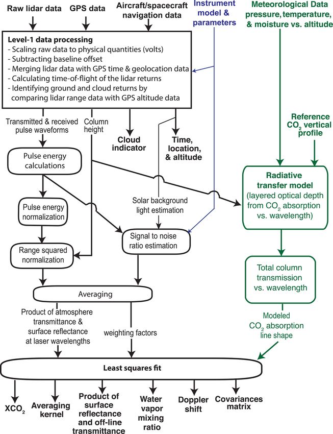
manathan et al., 2013, 2015, 2018). This paper gives a com- 3 Lidar signal processing and atmosphere modeling
plete description of the algorithm, the mathematical deriva-
tions, signal processing techniques, estimation error, and av- An overview of the retrieval algorithm for lidar data is shown
eraging kernel. An example of using the algorithm to analyze in Fig. 3. The initial processing consists of (a) processing
measurements from the airborne CO2 Sounder lidar is also the stored lidar data to estimate ranges to the reflecting sur-
presented. faces and form a series of atmosphere transmission measure-
ments across the CO2 absorption line; (b) generating a CO2
absorption line shape from the radiative transfer model and
2 Measurement approach meteorological data at the time and location of lidar measure-
ments; and (c) performing a least-squares fit of the modeled
The measurement geometry for the CO2 Sounder lidar is line shape function to the measurements to solve for XCO2
shown in Fig. 1. The lidar transmits laser pulses toward nadir, and other parameters.
and its receiver telescope collects the optical signal backscat-
tered from the atmosphere and the surface. Figure 2 shows a 3.1 Lidar signal processing
block diagram of the airborne CO2 Sounder lidar, which was
developed as an airborne demonstrator for NASA’s planned The signal waveforms are first corrected for the detector
Active Sensing of CO2 Emissions over Nights, Days, & Sea- baseline offset and other instrument characteristics and then
sons (ASCENDS) mission (Kawa et al., 2018). The laser scaled to the received optical signal power. The pulse ener-
Atmos. Meas. Tech., 14, 3909–3922, 2021 https://doi.org/10.5194/amt-14-3909-2021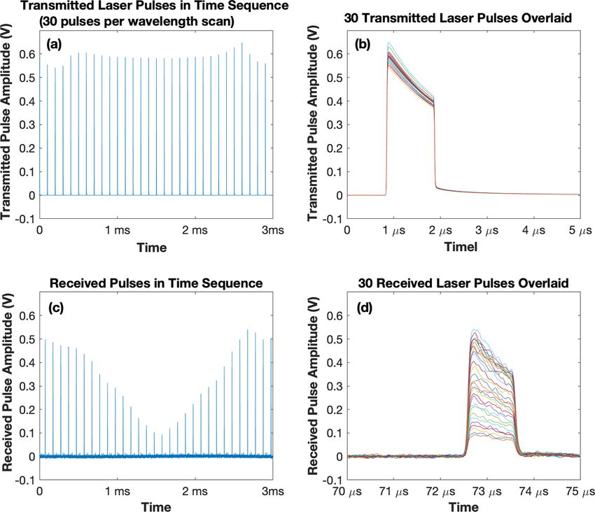
X. Sun et al.: Retrieval algorithm for XCO2 from lidar measurements                                                             3911

Figure 1. Illustrations of the CO2 Sounder lidar measurement geometry and received signal at a single laser wavelength.

Figure 2. Block diagram of the airborne CO2 Sounder lidar.

gies from the scattering surfaces are calculated by integrat-          from the cloud tops are usually sufficient for XCO2 retrievals
ing the received pulse waveforms over the pulse width in-              (Mao et al., 2018). For thin clouds and aerosols, the laser
terval. The relative atmosphere transmittances for all laser           pulses can often reach the ground surface and be received
wavelengths are calculated by dividing the received pulse en-          at the lidar with sufficient energy to allow useful XCO2 re-
ergies by the transmitted ones and then multiplying by the             trievals. The signal waveform before ground return can be
square of the range from the lidar to the reflecting surface.          averaged to obtain the atmospheric backscatter profiles at the
The signal-to-noise ratio (SNR) of the atmospheric transmit-           laser wavelength, which gives information about the heights
tances at each wavelength is estimated based on the received           and densities of thin clouds and aerosols (Allan et al., 2019).
signal energy, the estimated background noise, and the de-
tector noise. Finally, a least-squares fit of the modeled line         3.2   Model for the lidar signals
shape to the lidar measurements is used to estimate XCO2
along with the other parameters.                                       The average signal pulse energy reflected from the scattering
   The lidar returns from clouds are identified by compar-             surface can be calculated from the lidar equation (McMana-
ing the elevations of the lidar returns, namely aircraft alti-         mon, 2019), as
tude minus the lidar range, to the surface elevation from ei-
ther the onboard radar measurements or a digital elevation
                                                                                                   rs Ar
model (DEM). For dense clouds, the laser energies reflected            Er (λ) = Et (λ) · TA2 (λ)     ·   · ηr ,                   (1)
                                                                                                   π R2

https://doi.org/10.5194/amt-14-3909-2021                                                  Atmos. Meas. Tech., 14, 3909–3922, 2021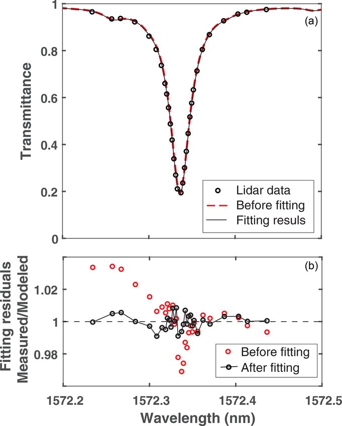
3912                                                  X. Sun et al.: Retrieval algorithm for XCO2 from lidar measurements

                                                                   3.3   Model for the CO2 absorption line shape

                                                                   The total atmospheric transmission from the lidar to the sur-
                                                                   face can be written as

                                                                   TA2 (λ) = TCO
                                                                              2
                                                                                 2
                                                                                   (λ) · Tw2 (λ) · To2 .                       (3)

                                                                   Here, TCO 2 (λ) and T 2 (λ) are the two-way atmospheric
                                                                               2            w
                                                                   transmissions of CO2 and water vapor at laser wavelength
                                                                   λ. The term To2 accounts for the transmission of aerosols
                                                                   and other particles, which are independent of the laser wave-
                                                                   length. To2 is often called the offline atmospheric transmis-
                                                                   sion. Note that Eq. (3) and the XCO2 measurement are for the
                                                                   atmosphere column from the lidar to the surface. This is dif-
                                                                   ferent from the passive remote sensing measurement where
                                                                   the incident light from the sun and the reflected light are at
                                                                   an angle and go through different atmosphere columns.
                                                                      To compute the transmission line shapes of CO2 and wa-
                                                                   ter vapor, the atmosphere is divided into a number of layers.
                                                                   The total transmission is modeled as the product of the in-
                                                                   dividual transmissions of all the layers traveled by the laser
                                                                   pulse. The layered transmission is calculated from the lay-
                                                                   ered radiative transfer atmospheric model, which takes into
                                                                   account the effects of the temperature, pressure, and humid-
                                                                   ity for each layer. The vertical profiles of temperature, pres-
                                                                   sure, and humidity are obtained from a meteorological anal-
                                                                   ysis model or, when possible, from in situ atmospheric mea-
                                                                   surements made during aircraft spiral-down maneuvers.
Figure 3. Flowchart of the XCO2 retrieval algorithm for the CO2
                                                                      The atmospheric transmissions of each layer for each of
Sounder lidar.
                                                                   the lidar wavelengths across the CO2 absorption line are cal-
                                                                   culated by using the Beer–Lambert law. The total two-way
where Er (λ) and Et (λ) are the received and transmitted laser     transmission due to CO2 can be written as
pulse energies at laser wavelength λ, TA (λ) is the one-way                         "
                                                                                          N2
                                                                                                                           #
atmosphere transmission at laser wavelength λ, rs is the dif-        2
                                                                   TCO2 (λi ) = exp −2
                                                                                         X
                                                                                              ρCO2 Hj σCO2 Hj , λi 1Hj , (4)
fuse surface reflectance to the laser beam, Ar is the light col-                           j =1
lecting area of the receiver telescope, R is the range from the
lidar to the scattering surface (the column height), and ηr is     where i = 1, 2, . . ., N1 is the index for the laser wavelengths
the receiver optical transmission efficiency.                      with N1 the total number of laser wavelengths used in the
   The product of the surface reflectance and the two-way          lidar measurements, j = 1, 2, . . ., N2 is the index for the at-
atmospheric transmission can be calculated from the received       mospherelayer with N2 the total number atmospheric layers,
laser pulse energy after correcting for the range as               ρCO2 Hj is the molecular density of CO2 for the j th layer,
                                                               Hj is the average altitude of the j th layer, and σCO2 Hj , λi
             2          π        Er (λ) 1                          is the absorption cross section of a CO2 molecule in the j th
y (λ) = rs TA (λ) =                    ·      .              (2)
                       Ar η r    Et (λ) R 2                        layer at the ith wavelength.
                                                                      Here we assumed that the laser wavelengths are known
The term in the parentheses of the right-hand side of Eq. (2)
                                                                   precisely and the laser spectral line width is much narrower
is a constant related to the lidar receiver. The telescope di-
                                                                   than the CO2 absorption line width. For the CO2 Sounder li-
ameter and overall optical transmission are measured in the
                                                                   dar, the laser is step locked to an onboard CO2 gas cell with
lab. The optical transmission can also be calibrated in flight
                                                                   fixed frequency offsets in each scan. The frequency accuracy
by flying over an area where the surface reflectance and the
                                                                   is < 1 MHz peak to peak, and the line width is about 30 MHz
atmospheric transmission are known from independent mea-
                                                                   (Numata et al., 2012), which are small compared to the CO2
surements. The term in brackets consists of variables mea-
                                                                   absorption line width. It has been shown that for lidar mea-
sured by the lidar.
                                                                   surements of XCO2 such small laser frequency deviations
                                                                   are negligible compared to other noise sources (Chen et al.,
                                                                   2012, 2014, 2015, 2019).

Atmos. Meas. Tech., 14, 3909–3922, 2021                                               https://doi.org/10.5194/amt-14-3909-2021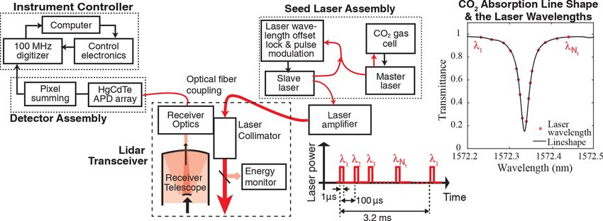
X. Sun et al.: Retrieval algorithm for XCO2 from lidar measurements                                                          3913

   The modeled optical transmission due to CO2 can also be       is used for the vertical grid coordinate for any of the profiles.
expressed in terms of the optical depth (OD) defined as the      The surface pressure and surface height are horizontally in-
absolute value of the logarithm of the one-way atmospheric       terpolated from the model.
transmission, as                                                    Since the power and size of the CO2 Sounder lidar are
  2
                                                               limited, there is a limit to the number of laser wavelengths
TCO 2
      (λi ) = exp −2ODCO2 (λi )                         (5)      which can be used to sample the XCO2 absorption line at a
and                                                              given rate and maintain adequate SNR at each wavelength.
                                                                 Although Ramanathan et al. (2018) showed a few additional
                N2
                X                                                parameters about the CO2 absorption line shape may be re-

ODCO2 (λi ) =          ρCO2 Hj σCO2 Hj , λi 1Hj                  trieved, they provide only limited information about the ver-
                j =1
                                                                 tical profile of CO2 mixing ratio. Therefore, we choose to
                N2
                X                                                retrieve a single scale factor for a reference profile, similar to

            =          1ODCO2 Hj , λi ,                    (6)   the profile scaling used in passive remote sensing (Borsdorff
                j =1                                             et al., 2014). Here the reference profile is obtained from the
where ODCO2 (λi ) is the column OD at wavelength λi and          radiative transfer model and meteorological data described
               P    N2                                        above. A least-squares method is used to solve for the scale
1ODCO2 Hj , λi =        ρCO2 Hj σCO2 Hj , λi 1Hj is the          factor that minimizes the error between the line shape model
                         j =1                                    and the lidar-sampled CO2 absorption line shape at all laser
OD of the atmosphere layer due to CO2 absorption at wave-        wavelengths. This retrieval method assumes that the modeled
length λi and altitude Hj .                                      line shape is accurate. In practice, there may be differences
   The molecular density of CO2 for the j th layer can be ex-    between the model and the actual line shape which could
pressed as                                                       cause biases in the solutions. However, if the modeling er-

ρCO2 Hj = XCO2 Hj ρair Hj ,

                                                           (7)   ror is random, the approach of using the lidar’s sampling of
                                                               the line at multiple wavelengths and using a line fit tends to
where XCO2 Hj is the CO2 mixing ratio and ρair Hj is             average out the effect of the discrepancies.
the dry-air molecular density at altitude Hj .                      Using the scale factor, the OD which is attributable to the
   In our XCO2 retrieval algorithm the layered OD is cal-        CO2 absorption can be written as
culated by using the HITRAN 2008 spectroscopy database                                N2
(Rothman et al., 2009) and the Line-By-Line Radiative
                                                                                      X
                                                                 ODCO2 (λi ) ≈ αCO2          XCO2 a Hj ρair Hj
Transfer Model (LBLRTM) V12.1 (Clough et al., 1992;                                   j =1
Clough and Iacono, 1995), for a given CO2 mixing ratio and
                                                                              × σCO2 Hj , λi 1Hj = αCO2 ODCO2 a (λi ) , (8)
meteorological vertical profiles at the time and location of
the lidar measurement.                                           where αCO2 is the scale factor, XCO2 a Hj is the a pri-
   The atmospheric pressure, temperature, and water vapor        ori (initial guess) CO2 mixing ratio at altitude Hj , and
can cause shifts and broadening of the CO2 absorption line,      ODCO2 a (λi ) is the a priori total column OD attributed to
which affects the cross sections at measured wavelengths.        CO2 absorption. The atmospheric transmission due to CO2
The LBLRTM software incorporates these effects and com-          absorption can now be approximated as
putes a numerical line shape function in OD at the given           2

                                                                 TCO   (λi ) ≈ exp −2αCO2 ODCO2 a (λi ) .                (9)
altitude of each layer. For the airborne data retrievals, me-        2

teorological data are obtained from the near-real-time for-
ward processing of the Goddard Modelling and Assimila-           4   Solving for XCO2 from the lidar measurements via a
tion Office (GMAO) FP system, the Goddard Earth Ob-                  least-squares fit
serving System Model, Version 5 (GEOS-5) (Rienecker et
al., 2011). The data are drawn from the eight-per-day ana-       The column XCO2 and several other variables are solved
lyzed fields on the full model grid (0.25 × 0.3125◦ × 72 lay-    simultaneously from a least-squares fit of the modeled line
ers, inst3_3d_asm_Nv files). The GEOS-5 data are used for        shape to the lidar measurements. One variable is the Doppler
the meteorological conditions for the retrievals at the times    shift in the wavelengths of the received signal, which occurs
and places where the airborne in situ profile measurements       when measuring at non-nadir angles from a moving platform.
are not available. For analysis of our airborne campaign         Another parameter being solved for is the product of the sur-
measurements, the GEOS-5 data were used primarily ex-            face reflectance and the two-way offline atmospheric trans-
cept during the spiral maneuvers. We extract the nearest-in-     mission. For the CO2 line at 1572.33 nm and under high hu-
time latitude–longitude interpolated meteorological sound-       midity, there is a weak isotopic water vapor absorption fea-
ings from the GEOS-5 data every minute at regular positions      ture on the left wing of the CO2 absorption line. The retrieval
along the flight’s ground tracks. The 42 lowest analysis lev-    algorithm can resolve this absorption feature to avoid caus-
els are used for each profile location. The analyzed pressure    ing biases in the retrieved XCO2 . For our airborne lidar, there

https://doi.org/10.5194/amt-14-3909-2021                                           Atmos. Meas. Tech., 14, 3909–3922, 2021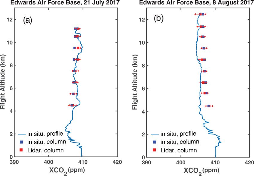
3914 X. Sun et al.: Retrieval algorithm for XCO2 from lidar measurements
is also a small linear trend (slope) in the received laser pulse where
energy as a function of the wavelength. The primary cause
f 0 (λ1 )
of this trend is the residual error from modeling the uneven ..
F0 = F (S0) =
spectral response of the receiver optics, especially the optical .
bandpass filter. Since the bandpass spectral shape can change f 0 λN1
slightly with temperature and time, the retrieval also solves
for this residual slope. with f (λi ) equal to Eq. (10) evaluated at the initial value of
The least-squares fit may be formulated by expressing the the parameter set.
lidar measurement data in matrix form, Y, a single column Substituting Eq. (12) into Eq. (11) and defining 1Y =
matrix with elements yi given by Eq. (2). The parameter to (Y − F0) and 1S = S − S0, the loss function can now be ap-
be solved for, S = {sk }, is expressed as a N3 ×1 matrix. In our proximated as
case N3 = 5, where each element is defined as s1 = rs To2 is T
∂F (S)
the product of the surface reflectance and the two-way atmo- J (Y, S) ≈ 1Y − |S=S0 1S
sphere transmission at offline wavelength, s2 = αCO2 is the ∂S
scale factor for the XCO2 line shape function, s3 = αwater is ∂F (S)
× W 1Y − |S=S0 1S . (13)
the scale factor for the water vapor line shape function, s4 is ∂S
the linear slope of the receiver spectral response, and s5 is the
Doppler shift of the received signal wavelengths. For mathematical convenience, we normalize the lidar mea-
The modeled atmospheric transmission given in Eq. (9) surements with respect to their initial estimate and define a
can be expressed as a single column matrix, F (S), called a new variable:
forward model, with each element equal to 1y (λi )
1y1 (λi1 ) = . (14)
f 0 (λi )
fi (S) = rs TA2 (λi , S)
h
2
ih
2
i A diagonal matrix IO can be defined with each element equal
≈ s1 s2 TCO 2
(λ i + s5 ) s 3 Twater (λ i + s5 ) to 1/f 0 (λi ). The loss function can be rewritten using the
× η0 (λi + s5 , s4 ) , (10) identity matrix I ≡ IO I−1 −1
O ≡ IO IO , as
T
where TA2 (λ, S) is the atmosphere transmission defined in
∂F (S)
J (Y, S) ≈ 1Y − |S=S0 1S IO I−1
O
Eq. (1) but expressed as a function of both the laser wave- ∂S
length and the parameters to be solved, and η0 (λ, s4 ) is the ∂F (S)
normalized receiver optical transmission as a function of the × W I−1
O I O 1Y − |S=S0 1S
∂S
wavelength and the slope of the linear trend of the receiver T
spectral response. Here we also included the term for the wa- ∂F1 (S)
= 1Y1 − 1S
ter vapor. ∂S
A scalar-valued loss function can be defined as the sum of
∂F1 (S)
squared differences between the lidar measurement data and × W1 1Y1 − 1S , (15)
∂S
the model, as
where 1Y1 = IO 1Y, F1 (S) = IO F (S), and W1 = I−1 O WIO .
J (Y, S) = [Y − F(S)]T W [Y − F(S)]
The use of the above normalization greatly simplifies the
N1
X 2 mathematical derivation as well as the data processing since
= wi,i y (λi ) − fi (S) , (11) it cancels out the exponential terms in the derivatives of F (S).
i=1
However, this technique can only be used when the values
where [Y − F(S)] is an N1 × 1 matrix and W is a N1 × N1 of the forward model f (λi ) are not approaching zero at all
diagonal matrix for weighting factors used in the fit. The sampling wavelengths.
weighting factors are chosen to balance the contributions The loss function given in Eq. (15) is of the same form
from the measurements at different laser wavelengths that as that of a linear least-squares fit with measurement data
have different SNRs. The least-squares fit finds the param- 1Y1 and weighting factor W1. The derivative of the function
eter set that minimizes the loss function. F1 (S), which is often referred to as the Jacobian, is given by
For small changes in XCO2 and for high SNR lidar mea-
∂ [F1 (S)]
surements, Eq. (11) can be linearized by the first two terms K= |S=S0 . (16)
of its power series expansion about initial estimates of the ∂S
parameter values, S0. The function F (S), also known as the For the CO2 Sounder lidar, each term of the Jacobian can
forward model, can then be approximated by be derived as ki,1 = ∂F(S) 1 1
s1 f 0(λi ) = hrs To2 i , same for all i =
∂F (S) 1, 2, . . ., N1 ; ki,2 = −2ODCO2 a (λi ), one for each laser wave-
F (S) ≈ F0 + |S=S0 (S − S0) , (12) length, i = 1, 2, . . ., N1 ; ki,3 , same as above but for water
∂S
Atmos. Meas. Tech., 14, 3909–3922, 2021 https://doi.org/10.5194/amt-14-3909-2021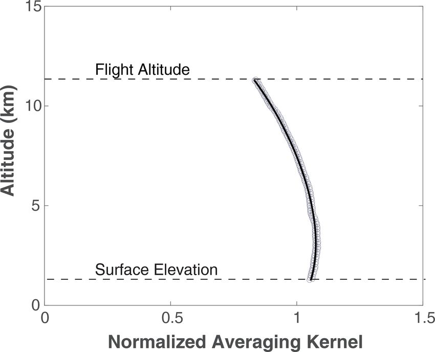
X. Sun et al.: Retrieval algorithm for XCO2 from lidar measurements                                                         3915

vapor; ki,4 = (λi − λc ), with λc the center wavelength of        where Gα is the row of the G matrix for calculating the
                                         2 (λ +1λ)−T 2 (λ )
                                        TCO
                                            2
                                              i     CO2 i         XCO2 scale factor and Kx is the Jacobian of the measure-
the CO2 line shape function; ki,5 ≈             1λ     ·
    1
                                                                  ment with respect to the layered CO2 mixing ratios, which is
  2    , with 1λ = 1 pm (or the expected average Doppler          an N1 × N2 matrix given by
hTCO (λi )i
    2
            2 (λ ) given by Eq. (4).
shift) and TCO 2
                  i                                                      ∂F(XCO2 )
   For measurement noise that is zero mean and follows            Kx =             .                                         (22)
                                                                          ∂XCO2
a Gaussian distribution, the optimal weighting factors are
given by the reciprocal of the variance of the measurement        Each term of Kx can be written according to Eqs. (2)–(4),
data (Bevington, 1969). In our case, the optimal weighting        (7), and (10), as
factors can be approximated as
                                                                  Kx (i, j ) = ρair Hj σCO2 Hj , λi 1Hj .
                1          f 0(λi )2     hy (λi ) i2
w1i,i =                  =             ≈
          var {1y1 (λi )} var {y (λi )} var {y (λi )}             The linear least-squares fit can also be iterated by correct-
                  2                                               ing for the Doppler shift of the received laser wavelengths of
        = SNR(λi ) ,                                      (17)
                                                                  the modeled line shape based on the solution from the previ-
where hy (λi )i is the average value of the lidar measurement     ous iteration. The Jacobian terms are recalculated about the
which is assumed to be close to the initial estimate f 0 (λi ).   updated linearization point in each iteration to improve the
Therefore, for each wavelength the weighting factors can be       results.
approximated by the SNR of the lidar measurement at that
wavelength. As mentioned earlier, the SNRs are calculated
                                                                  5   Evaluation of the retrieval algorithm using airborne
based on signal energy and background noise estimated from
                                                                      lidar data
received pulse waveforms.
   The XCO2 and other parameters can now be solved using          The algorithm described here was used to retrieve XCO2
a standard linear least-squares fitting method with the loss      from measurements of our 2017 airborne lidar campaign
function Eq. (15), Jacobian Eq. (16), and weighting factors       (Mao et al., 2019). The lidar and the airborne measurements
Eq. (17). The solutions can be obtained numerically using         have been described in detail in Abshire et al. (2018). Ta-
the pseudo inverse function, as                                   ble 1 lists the instrument parameters relevant to the XCO2
                                                                  retrieval. Here we show a few examples of using the re-
1Ŝ = G1Y1                                                (18)
                                                                  trieval algorithm on a data set collected during one of the
with G a N3 × N1 matrix, which is often called the gain ma-       2017 flights. We also show the retrieved XCO2 at different
trix and can be computed from the pseudo inverse function         altitudes in comparison to XCO2 calculated from the in situ
pinv (·) (Peters and Wilkinson, 1970), as                         measurements made during two spiral-down maneuvers.
                                                                     Figure 4 shows an example of a Level-1 data set from our
G = pinv KT pinv (W1) K KT pinv (W1) .

                                                        (19)      2017 airborne campaign. It shows 30 transmitted pulse wave-
                                                                  forms and the corresponding received pulse waveforms aver-
The pseudo inverse matrix function can be found in the MAT-       aged over 32 laser wavelength scans. The decrease (tilt) of
LAB software package and in other software tools.                 laser pulse amplitudes over the pulse width interval is caused
  The covariance of the parameters can be obtained from           by the depletion of energy stored in the laser gain media,
Eq. (18), as                                                      which does not affect the IPDA lidar measurements. The en-
                                                                ergies of the transmitted laser pulses at different wavelengths
cov 1Ŝ = Gvar (1Y1) GT ,                               (20)      fluctuate by a few percent, which is monitored and corrected
                                                                  for in the signal processing. The tails in the transmitted pulse
with var (1Y1) a diagonal matrix with each element the re-        waveforms shown in Fig. 4b are caused by an artifact of the
ciprocal of the corresponding element in Eq. (17). The co-        laser monitor detector, which is different from the one used
variance matrix cov(1Ŝ) is in general not a diagonal matrix      in the receiver. The amplitudes and energies of the received
even though var (1Y1) is a diagonal matrix.                       laser pulse waveform plotted in Fig. 4c clearly show the CO2
   The variances of the estimated parameters are given by         absorption near the center of the wavelength scan. The XCO2
the diagonal elements of cov(1Ŝ). However, variance is only      retrieval is carried out at 1 Hz, during which the host aircraft
one of the criteria of the XCO2 retrieval. There can still be     typically travels about 200 m.
a bias in the estimated parameters if there is a mismatch be-        For the least-squares fit the weighting factor for each
tween the measurements and the modeled line shape.                wavelength is the square of the SNR of the lidar-detected
   The total column averaging kernel can be calculated as         signals at that wavelength. The SNRs are estimated from the
(Borsdorff et al., 2014)                                          received lidar signal as (Gagliardi and Karp, 1995)
A = Gα Kx ,                                               (21)

https://doi.org/10.5194/amt-14-3909-2021                                            Atmos. Meas. Tech., 14, 3909–3922, 2021
3916 X. Sun et al.: Retrieval algorithm for XCO2 from lidar measurements
Table 1. The airborne CO2 Sounder lidar instrument parameters.
Instrument parameters Values
Laser
Pulse energy 25 µJ
Wavelength scan range 1572.235–1572.440 nm
Number of wavelengths 30 (see Fig. 5)
Wavelength accuracy 0.008 pm (1 MHz)
Spectral line width < 0.247 pm (30 MHz)
Pulse width 1 µs
Pulse rate 10 kHz
Divergence angle 0.43 mrad (4.3 m laser spot size on ground from a 10 km altitude)
Receiver optics
Telescope size 20 cm diameter
Field of view 0.50 mrad
Optical filter bandwidth 1.4 nm
Total optical transmission 81.3%
Detector and receiver electronics
Quantum efficiency, including fill factor 69 %
Responsivity 6.39 × 10⁸ V /W
Noise equivalent power (NEP), 16 pixels combined 6.9 fW Hz−1/2
Signal sample rate 100 MHz, 16 bits
Integration time for each XCO2 retrieval 1s
Data recording duty cycle 90 %
Figure 4. Sample pulse waveforms of the airborne CO2 Sounder lidar taken during the flight of 21 July 2017 00:30:00 UTC (local time
20 July 2017 17:30:00). (a) The 30 transmitted laser pulse waveforms in a wavelength scan averaged over 32 repeated scans. (b) Overlay of
the 30 transmitted pulse waveforms. (c) The corresponding received laser pulse waveforms reflected from the ground surface showing the
lidar sampled CO2 absorption. (d) An overlay of the received pulse waveforms for all 30 laser wavelengths.
Atmos. Meas. Tech., 14, 3909–3922, 2021 https://doi.org/10.5194/amt-14-3909-2021X. Sun et al.: Retrieval algorithm for XCO2 from lidar measurements 3917
SNR (λi ) =
ηd hns (λi )i
r h i . (23)
τs τs τs hna i2
Fd ηd hns (λi )i + 1 + τb hnb i + 1 + τb hnd i + 1 + τb hGd i2
Here hns (λi )i is the average number of received signal pho-
tons per pulse at wavelength λi , hGd i is the average gain
of the avalanche photodiode (APD) detector, ηd is the APD
quantum efficiency, Fd is the APD gain excess noise factor,
τs is the integration time for the signal pulse, τb is the in-
tegration time for the background and dark noise, hnb i and
hnd i are the average number of background photons and de-
tector dark counts integrated over the pulse interval, and hna i
is the standard deviation of the preamplifier noise in terms of
equivalent number of photoelectrons. The signal here refers
to the number of detected signal photons, which is equal to
the number of the detected photons minus the number of de-
tected background photons.
The laser speckle noise term (Goodman, 1965, 1975) is
not included in Eq. (23) since it is not a major noise source Figure 5. (a) An example of a CO2 absorption line shape sampled
for our airborne lidar measurements at nominal flight alti- by the airborne lidar (black circles) for 1 s averaging time and the
tude. This is because of the large number of speckle cells in models before and after the fit (red and black lines). (b) Differences
the laser footprint and the numerical averaging of the 30 re- (the residuals) between the lidar measurement and the model at the
ceived laser pulses for each XCO2 retrieval. Laser speckle lidar wavelengths before (in red circles) and after (in black circles)
noise is also not expected to be a major noise source for the the least-squares fit for the data set shown in Fig. 4. The retrieved
space version of the CO2 Sounder lidar being developed at scale factor was αXCO2 ≈ 1.025 (i.e., 410 ppm retrieved vs. 400 pm
NASA GSFC (see chap. 5 of Kawa et al., 2018) since the ef- assumed).
fects of spatial and numerical averaging are similar. The ef-
fects of errors in the meteorological data used to construct the
line shape model of CO2 are also not considered in Eq. (23).
We are currently conducting computer simulations to quan-
tify the effect of meteorological data errors, and the results
will be reported in a separate publication.
For the XCO2 retrieval, the average number of received
signal photons is estimated from the received pulse wave-
form. This is obtained by first integrating the received pulse
waveform from the detector in volts, dividing the result by
the detector responsivity in volts per watt, and the photon en-
ergy in joules. The average number of background noise pho-
tons is estimated from the average surface reflectance, offline
atmosphere transmission, nominal sunlight irradiance on the Figure 6. The averaging kernel from the retrieved data (open cir-
surface, and receiver optics model. All other parameter val- cles) and the fourth-order polynomial fit with altitude (solid black
ues in Eq. (23) are instrument related and can be found in curve) from the measurement data shown in Fig. 5.
Abshire et al. (2018).
Figure 5 shows the CO2 absorption line shape sampled by
the lidar along with that from the forward model which as- ments and the model after the least-squares fit are also plotted
sumes a constant XCO2 vertical profile of 400 parts per mil- in Fig. 5. The averaging kernel is calculated based on Eq. (21)
lion (ppm). It also shows the placement of laser wavelengths for each fit of 1 s lidar measurement data. Figure 6 shows the
across the CO2 absorption line. One laser wavelength (the normalized averaging kernel with respect to its average value
second from the left) was placed at a secondary absorption over the atmosphere column height and a fourth-order poly-
feature due to deuterated water vapor (HDO). Three wave- nomial fit for the data shown above.
lengths were placed on the wings of the CO2 absorption line. Figure 7 shows the results of the retrieval using the al-
The rest were roughly equally spaced in OD along the ab- gorithm described above from the airborne CO2 Sounder
sorption line. The residual differences between the measure- lidar measurements made on 21 July 2017 starting at
https://doi.org/10.5194/amt-14-3909-2021 Atmos. Meas. Tech., 14, 3909–3922, 20213918 X. Sun et al.: Retrieval algorithm for XCO2 from lidar measurements
Figure 8. The column XCO2 from the aircraft to the surface re-
trieved from the lidar measurements (red squares) compared to that
computed from the in situ measurements (blue squares) during the
spiral-downs on (a) 21 July 2017, near the end of the data seg-
ment shown in Fig. 7 and (b) 8 August 2017. The error bars on
the red squares represent mean and the standard deviation of the li-
dar measurement results binned into 1 km layers. The blue squares
are the column mixing ratio integrated from the readings of the AV-
OCET gas analyzer from the flight altitude to the surface. For the
spiral-down comparisons, the median differences (biases) between
the retrieved lidar and column in situ measurements are 0.72 ppm
for 21 July and 0.16 ppm for 8 August 2017.
Figure 7. The results of the retrieval sequence from the airborne
CO2 Sounder lidar data starting at 21 July 2020 00:30:00 UTC for
820 s over Edwards Air Force Base in California. These are all
based on 1 s receiver integration time. They are, from top down, spiral-down path from 12 to 4 km over Edwards Air Force
(a) the aircraft altitude, the lidar range from the laser pulse time Base for the flight on 21 July 2017 and for that on 8 Au-
of flight, the surface elevation computed from the onboard GPS re- gust 2017. The in situ profiles were measured by an updated
ceiver, and the lidar range; (b) the retrieved surface reflectance times version of the AVOCET gas analyzer on board the airplane
the two-way offline atmospheric transmission; (c) offline SNR cal- (Vay et al., 2011). The in situ XCO2 is calculated from the
culated from Eq. (23); (d) the retrieved XCO2 ; and (e) standard airplane altitude to the ground and is obtained by integrat-
deviation of the retrieved XCO2 from the covariance matrix. The ing the CO2 profile from the in situ measurements weighted
airplane velocity was about 200 m s−1 . The distance covered by the by the lidar’s averaging kernel. The XCO2 retrieved from the
data shown in the plot is about 164 km. lidar measurements agrees with that calculated from the in
situ measurements at all airplane altitudes above 4 km. Be-
low 4 km, the laser beam no longer completely overlaps the
00:30:00 UTC for 820 s. The data consist of about a 500 s field of view of the receiver, and the total CO2 absorption
segment measured at a nearly constant aircraft altitude fol- (line depth) becomes small. The lidar measurements are not
lowed by about 300 s of measurements in a spiral descent. calibrated at such a low altitude.
The last part of the flight was near Edwards Air Force Base,
CA, and the surface elevation was nearly constant for the last
500 s. The ground surface over this stretch of the flight was 6 Discussion
dry desert, and the sky was visually clear at the time. The re-
trieved XCO2 over this period was steady with a slow down- 6.1 Biases in the retrieved XCO2
ward trend. The root-mean-squared (rms) variation in the re-
trieved XCO2 from 2100 to 2300 s was 0.67 ppm, which in- Although the least-squares-fit method minimizes the sum of
cludes both the fitting error and the actual XCO2 variation squared errors between the modeled line shape and the li-
along the flight path. By comparison, the estimated stan- dar measurements, it does not guarantee minimum biases in
dard deviation from the retrieval covariance matrix was about the estimated parameters. The variance of the solutions can
0.35 ppm, as shown in Fig. 7e. approach zero as the SNR increases, as shown in Eq. (18),
Figure 8 shows the retrieved XCO2 compared to that cal- but biases remain. For example, if the actual CO2 absorption
culated from in situ measurements as the airplane flew in a line shape does not match that of the model, the retrieved
Atmos. Meas. Tech., 14, 3909–3922, 2021 https://doi.org/10.5194/amt-14-3909-2021X. Sun et al.: Retrieval algorithm for XCO2 from lidar measurements 3919
results can be biased regardless of the SNR. Therefore, it is retrieved values, which limits the benefit. One example is to
important to model the atmosphere and the absorption spec- divide the atmosphere into a few layers, each with its own
troscopy accurately and avoid systematic errors. line shape function and scale factor, to obtain some informa-
tion about the vertical distribution of XCO2 . The results from
6.2 Choice of laser wavelengths the least-squares fit for the XCO2 for the layers, however, are
correlated, and the errors from the fits are usually too large
The choice of the lidar laser wavelengths is a trade-off among to be useful (Chen et al., 2014). A singular value decomposi-
several factors. The total number of laser wavelengths has to tion (SVD) method has also been used to extract a few more
be greater than the number of parameters to be solved for in parameters about the line shape without the need for an a
the retrieval; however, the total average laser output power priori vertical XCO2 profile (Ramanathan et al., 2018). For
is fixed. Using fewer wavelength samples allows improve- measurement with high SNR, the SVD method can retrieve
ment of the SNR for each sample but provides fewer con- some characteristics of the line shape, such as the line width,
straints to the curve fit. More wavelength samples lower the and provide some constraints about the vertical distribution
SNR at each wavelength but allow us to solving for more pa- of XCO2 .
rameters and helps to reduce the bias in the XCO2 retrieval.
There is also an advantage to select the laser wavelengths
to be symmetrically distributed about the line center since 7 Conclusion
it reduces the effect of the nonuniformity in the receiver’s
spectral response (Chen et al., 2019). Finally, the laser wave- An algorithm to retrieve XCO2 has been developed for mea-
lengths should not be placed where the CO2 absorption is too surements from a pulsed multi-wavelength IPDA lidar. The
high, e.g., OD > 1.5, since the received signal level becomes retrieval algorithm uses a least-squares fit of the line shape
too low to contribute to the retrieval. function derived from a multi-layer atmosphere radiative
The airborne CO2 Sounder lidar mostly used 30 wave- transfer model based on meteorological data to the line shape
lengths with four offline, four near the center of the peak sampled by the lidar measurements. In addition to XCO2 ,
absorption up to OD = 1.2, one on the water vapor peak ab- the algorithm simultaneously solves for the product of the
sorption, and the rest approximately uniformly distributed in surface reflectance and the offline atmosphere transmission,
OD (Abshire et al., 2018). This choice of the laser wave- Doppler shift of the received laser signals, a secondary water
lengths produced measurement precisions < 1 ppm and bi- vapor mixing ratio (if present), and a linear trend of the lidar
ases < 1 ppm. Abshire et al. (2018) also report airborne mea- receiver non-uniformity in its spectral response. Since it can
surements made using 15 laser wavelengths that showed no accurately retrieve XCO2 as these conditions vary, this ap-
apparent difference in the XCO2 measurements to those us- proach provides a more robust measurement of XCO2 com-
ing 30 wavelengths for the otherwise same instrument con- pared to IPDA lidar that uses only online and offline wave-
figuration. lengths. The retrieval algorithm has been used successfully
The retrieval algorithm described in this paper could also in the data processing of the NASA GSFC multi-wavelength
be used for the online and offline dual-wavelength IPDA lidar pulsed IPDA lidar from its 2016 and 2017 airborne cam-
to retrieve XCO2 and the product of surface reflectance and paigns. The algorithm may also be used for retrievals for
two-way atmosphere transmission. The solution to the least- multi-wavelength lidars that target other atmospheric gases,
squares fit for the two parameters can be derived analytically such as CH4 .
and becomes the same as those reported earlier (Abshire et
al., 2010). The standard deviation of the retrieved XCO2 at a
given average laser power can be lower compared to that of a Code availability. An IDL (Interactive Data Language) version of
multi-wavelength IPDA lidar, depending on the placement of the software code for the least-squares fit will be posted at the same
the online wavelength. However, the Doppler shift, water va- website by 1 July 2021 or contact the author xiaoli.sun-1@nasa.gov.
por content, and the receiver spectral response would have to
be obtained and corrected well enough to avoid XCO2 bias.
The results would be much more sensitive to uncertainties in Data availability. The retrieved XCO2 from the 2017 airborne
lidar measurements is available from the NASA Airborne Science
the CO2 absorption line shape.
Data for Atmospheric Composition website, https://www-air.
larc.nasa.gov/cgi-bin/ArcView/ascends.2017#ABSHIRE.JAMES/
6.3 Number of parameters to retrieve (NASA Langley Research Center, 2020).
It is possible to use the least-squares fit to solve for more
parameters of the CO2 absorption line and lidar instrument, Author contributions. XS led the writing of the manuscript and pro-
as long as the information content of the lidar measurements vided the mathematical formulation of the retrieval algorithm. JBA
supports them. However, solving for more parameters, espe- was the principal investigator of the CO2 Sounder lidar develop-
cially when they are correlated, increases the variance in the ment and led the 2016 and 2017 ASCENDS airborne campaigns.
https://doi.org/10.5194/amt-14-3909-2021 Atmos. Meas. Tech., 14, 3909–3922, 20213920 X. Sun et al.: Retrieval algorithm for XCO2 from lidar measurements
AR developed the retrieval algorithm and the data processing soft- Amediek, A., Ehret, G., Fix, A., Wirth, M., Büdenbender, C.,
ware. SRK and JM developed the atmospheric model used in the Quatrevalet, M., Kiemle, C., and Gerbig, C.: CHARM-F: A
least-squares fit for the airborne measurement data processing. JM new airborne integrated-path differential-absorption lidar for car-
also processed and analyzed the 2017 airborne measurement data. bon dioxide and methane observations: measurement perfor-
mance and quantification of strong point source emissions, Appl.
Optics, 56, 5182–5197, https://doi.org/10.1364/AO.56.005182,
Competing interests. The authors declare that they have no conflict 2017.
of interest. Bevington, P. R.: Data Reduction and Error Analysis for the Physi-
cal Science, chap. 6, McGraw-Hill, New York, USA, 1969.
Borsdorff, T., Hasekamp, O. P., Wassmann, A., and Landgraf,
Acknowledgements. We thank the CO2 Sounder lidar team at J.: Insights into Tikhonov regularization: application to trace
NASA GSFC for the development of the lidar, conducting the air- gas column retrieval and the efficient calculation of total
borne campaigns, and collecting the measurement data. We also column averaging kernels, Atmos. Meas. Tech., 7, 523–535,
thank Joshua P. Digangi for the AVOCET measurements, Julie https://doi.org/10.5194/amt-7-523-2014, 2014.
Nicely for updating and testing the software for the XCO2 retrieval, Campbell, J. F., Lin, B., Dobler, J., Pal, S., Davis, K., Obland, M. D.,
and Jeffrey Chen for many technical discussions about XCO2 re- Erxleben, W., McGregor, D., O’Dell, C., Bell, E., Weir, B., Fan,
trievals. T-.F., Kooi, S., Gordon, I., Corbett, A., and Kochanov, R.: Field
evaluation of column CO2 retrievals from intensity-modulated
continuous-wave differential absorption lidar measurements
during the ACT-America campaign, Earth Space Sci., 7,
Financial support. This research has been supported by the NASA
e2019EA000847, https://doi.org/10.1029/2019EA000847, 2020.
Earth Sciences Technology Office (ESTO) and the NASA AS-
Chen, J. R., Numaa, K., and Wu, S. t.: Error reduction
CENDS Mission pre-formulation program.
methods for integrated-path differential-absorption li-
dar measurements, Opt. Express, 20, 15590–15609,
https://doi.org/10.1364/OE.20.015589, 2012.
Review statement. This paper was edited by Markus Rapp and re- Chen, J. R., Numata, K., and Wu, S. T.: Error reduction in re-
viewed by two anonymous referees. trieval of atmospheric species from symmetrically measured li-
dar sounding absorption spectra, Opt. Express, 22, 26055–26075,
https://doi.org/10.1364/OE.22.026055, 2014.
Chen, J. R., Numata, K., and We, S. T.: Impact of broadened
References laser line-shape on retrieval of atmospheric species from li-
dar sounding absorption spectra, Opt. Express, 23, 2660–2675,
Abshire, J. B., Riris, H., Allan, G. R., Weaver, C., Mao, J., Sun, https://doi.org/10.1364/OE.23.002660, 2015.
X., Hasselbrack, W. E., Kawa, S. R., and Biraud, S.: Pulsed Chen, J. R., Numata, K., and Wu, S. T.: Error analysis for lidar re-
airborne lidar measurements of atmospheric CO2 column ab- trievals of atmospheric species from absorption spectra, Opt. Ex-
sorption, Tellus B, 62, 770–783, https://doi.org/10.1111/j.1600- press, 27, 36487–36504, https://doi.org/10.1364/OE.27.036487,
0889.2010.00502.x, 2010. 2019.
Abshire, J. B., Riris, H., Weaver, C., Mao, J., Allan, G., Hassel- Clough, S. A. and Iacono, M. J.: Line-by-line calculation of atmo-
brack, W., and Browell, E. V.: Airborne measurements of CO2 spheric fluxes and cooling rates 2. Application to carbon dioxide,
column absorption and range using a pulsed direct-detection inte- methane, nitrous oxide and the halocarbons, J. Geophys. Res.-
grated path differential absorption lidar, Appl. Optics, 52, 4446– Atmos. 100, 16519–16535, https://doi.org/10.1029/95JD01386,
4461, https://doi.org/10.1364/AO.52.004446, 2013. 1995.
Abshire, J. B., Ramanathan, A., Riris, H., Mao, J., Allan, G. R., Clough, S. A., Iacono, M. J., and Moncet, J.: Line-by-line cal-
Hasselbrack, W. E., Weaver, C. J., and Browell, E. V.: Airborne culations of atmospheric fluxes and cooling rates: Application
measurements of CO2 column concentration and range using a to water vapor, J. Geophys. Res.-Atmos. 97, 15761–15785,
pulsed direct-detection IPDA lidar, Remote Sens., 6, 443–469, https://doi.org/10.1029/92JD01419, 1992.
https://doi.org/10.3390/rs6010443, 2014. Crisp, D., Pollock, H. R., Rosenberg, R., Chapsky, L., Lee, R. A.
Abshire, J. B., Ramanathan, A. K., Riris, H., Allan, G. R., Sun, M., Oyafuso, F. A., Frankenberg, C., O’Dell, C. W., Bruegge, C.
X., Hasselbrack, W. E., Mao, J., Wu, S., Chen, J., Numata, J., Doran, G. B., Eldering, A., Fisher, B. M., Fu, D., Gunson, M.
K., Kawa, S. R., Yang, M. Y. M., and DiGangi, J.: Airborne R., Mandrake, L., Osterman, G. B., Schwandner, F. M., Sun, K.,
measurements of CO2 column concentrations made with a Taylor, T. E., Wennberg, P. O., and Wunch, D.: The on-orbit per-
pulsed IPDA lidar using a multiple-wavelength-locked laser and formance of the Orbiting Carbon Observatory-2 (OCO-2) instru-
HgCdTe APD detector, Atmos. Meas. Tech., 11, 2001–2025, ment and its radiometrically calibrated products, Atmos. Meas.
https://doi.org/10.5194/amt-11-2001-2018, 2018. Tech., 10, 59–81, https://doi.org/10.5194/amt-10-59-2017, 2017.
Allan, G. R., Sun, X., Abshire, J. B., Riris, H., Hasslbrack, W. E., Dobler, J., Harrison, F., Browell, E., Lin, B., McGregor, D.,
Kawa, S. R. Numata, K., Mao, J., and Chen, J.: Atmospheric Kooi, S., Choi, Y., and Ismail, S.: Atmospheric CO2 column
backscattering profiles from the 2017 ASCENDS/ABoVE air- measurements with an airborne intensity-modulated continuous
borne campaign measured by the CO2 Sounder lidar, 2019 Fall wave 1.57 µm fiber laser lidar, Appl. Optics, 52, 2874–2892,
AGU Annual Meeting, 9–13 December 2019, San Francisco, https://doi.org/10.1364/AO.52.002874, 2013.
CA, USA, Paper A51M-2726, 2019.
Atmos. Meas. Tech., 14, 3909–3922, 2021 https://doi.org/10.5194/amt-14-3909-2021X. Sun et al.: Retrieval algorithm for XCO2 from lidar measurements 3921 Eldering, A., O’Dell, C. W., Wennberg, P. O., Crisp, D., Gunson, M. tion of atmospheric cO2 concentration measurements with R., Viatte, C., Avis, C., Braverman, A., Castano, R., Chang, A., a pulsed multi-wavelength IPDA lidar, 15th International Chapsky, L., Cheng, C., Connor, B., Dang, L., Doran, G., Fisher, Workshop on Greenhouse Gas Measurements from Space B., Frankenberg, C., Fu, D., Granat, R., Hobbs, J., Lee, R. A. M., (IWGGMS), 3–5 June 2019, Sapporo, Japan, Paper 5-5, Mandrake, L., McDuffie, J., Miller, C. E., Myers, V., Natraj, V., available at: https://www.nies.go.jp/soc/doc/Oral_Presentations/ O’Brien, D., Osterman, G. B., Oyafuso, F., Payne, V. H., Pol- Session5-6/5-5_iw15op_Jianping_Mao.pdf (last access: 14 May lock, H. R., Polonsky, I., Roehl, C. M., Rosenberg, R., Schwand- 2021), 2019. ner, F., Smyth, M., Tang, V., Taylor, T. E., To, C., Wunch, D., McManamon, P.: LiDAR, Technologies and Systems, chap. 3, SPIE and Yoshimizu, J.: The Orbiting Carbon Observatory-2: first 18 Press, Bellingham, USA, 2019. months of science data products, Atmos. Meas. Tech., 10, 549– Menzies, R. T., Spiers, G. D., and Jacob, J.: Airborne laser ab- 563, https://doi.org/10.5194/amt-10-549-2017, 2017. sorption spectrometer measurements of atmospheric CO2 col- Eldering, A., Taylor, T. E., O’Dell, C. W., and Pavlick, R.: umn mole fractions: source and sink detection and environmen- The OCO-3 mission: measurement objectives and expected tal impacts on retrievals, J. Atmos. Ocean Technol., 31, 404–421, performance based on 1 year of simulated data, Atmos. https://doi.org/10.1175/JTECH-D-13-00128.1, 2014. Meas. Tech., 12, 2341–2370, https://doi.org/10.5194/amt-12- NASA Langley Research Center: Airborne Science Data for Atmo- 2341-2019, 2019. spheric Composition, available at: https://www-air.larc.nasa.gov/ Gagliardi, R. M. and Karp, S.: Optical Communications, 2nd edn., cgi-bin/ArcView/ascends.2017#ABSHIRE.JAMES/ (last access: John Wiley and Sons, Hoboken, New Jersey, USA, 1995. 16 May 2021), 2020. Goodman, J. W.: Some effects of target-induced scintillation Numata, K., Chen, J. R., and Wu, S. T.: Precision and on optical radar performance, Proc. IEEE, 55, 1688–1700, fast wavelength tuning of a dynamically phase-locked https://doi.org/10.1109/PROC.1965.4341, 1965. widely-tunable laser, Opt. Express, 20, 14234–14243, Goodman, J. W.: Statistics properties of laser speckle patterns, in: https://doi.org/10.1364/OE.20.014234, 2012. Laser Speckle and Related Phenomena, edited by: Dainty, J. C., Peters, G. and Wilkinson, J. H.: The least squares prob- Spinger-Verlag, Berlin, Heidelbery, Germany, 9–75, 1975. lem and pseudo-Inverses, Comput. J., 13, 309–316, Han, G., Shi, T., Ma, X., Xu, H., Zhang, M., Liu, Q., https://doi.org/10.1093/comjnl/13.3.309, 1970. and Wei, G.: Obtaining gradients of XCO2 in atmosphere Ramanathan, A., Mao, J., Allan, G. R., Riris, H., Weaver, C. J., using the constrained linear least-squares technique and Hasselbrack, W. E., Browell, E. V., and Abshire, J. B.: Spectro- multi-wavelength IPDA LiDAR, Remote Sens., 12, 2395, scopic measurements of a CO2 absorption line in an open verti- https://doi.org/10.3390/rs12152395, 2020. cal path using an airborne lidar, Appl. Phys. Lett., 103, 214102, Jacob, J. C., Menzies, R. T., and Spiers, G. D.: Data processing and https://doi.org/10.1063/1.4832616, 2013. analysis approach to retrieve carbon dioxide weighted-column Ramanathan, A. K., Mao, J., Abshire, J., and Allan, G. mixing ratio and 2 µm reflectance with an airborne laser absorp- R.: Remote sensing measurements of the CO2 mixing ra- tion spectrometer, IEEE Trans. Geosci. Remote Sens., 57, 958– tio in the planetary boundary layer using cloud slicing 971, https://doi.org/10.1109/TGRS.2018.2863711, 2019. with airborne lidar, Geophys. Res. Lett., 42, 2055–2062, Kawa, S. R., Abshire, J. B., Baker, D. F., Browell, E. V., Crisp, https://doi.org/10.1002/2014GL062749, 2015. D., Crowell, S. M. R., Hyon, J. J., Jacob, J. C., Jucks, K. Ramanathan, A. K., Nguyen, H. M., Sun, X., Mao, J., Abshire, W., Lin, B., Menzies, R. T., Ott, L. E., and Zaccheo, T. S.: J. B., Hobbs, J. M., and Braverman, A. J.: A singular value Active Sensing of CO2 Emissions over Nights, Days, and decomposition framework for retrievals with vertical distribu- Seasons (ASCENDS): Final Report of the ASCENDS, Ad tion information from greenhouse gas column absorption spec- Hoc Science Definition Team, Document ID: 20190000855, troscopy measurements, Atmos. Meas. Tech., 11, 4909–4928, NASA/TP–2018-219034, GSFC-E-DAA-TN64573, available at: https://doi.org/10.5194/amt-11-4909-2018, 2018. https://www-air.larc.nasa.gov/missions/ascends/docs/NASA_ Refaat, T. F., Singh, U. N., Yu, J., Petros, M., and Ismail, S.: Double- TP_2018-219034_ASCENDS_ID1.pdf (last access: 14 May pulse 2 µm integrated path differential absorption lidar airborne 2021), 2018. validation for atmospheric carbon dioxide measurement, Appl. Kuze, A., Suto, H., Shiomi, K., Kawakami, S., Tanaka, M., Ueda, Optics, 55, 4232–4246, https://doi.org/10.1364/AO.55.004232, Y., Deguchi, A., Yoshida, J., Yamamoto, Y., Kataoka, F., Tay- 2016. lor, T. E., and Buijs, H. L.: Update on GOSAT TANSO- Refaat, T. F., Petros M., Singh, U. N., Antill, C. W., and Re- FTS performance, operations, and data products after more mus Jr., R. G.: High-precision and high-accuracy column dry-air than 6 years in space, Atmos. Meas. Tech., 9, 2445–2461, mixing ratio measurement of carbon dioxide using pulsed 2 µm https://doi.org/10.5194/amt-9-2445-2016, 2016. IPDA lidar, IEEE Trans. Geosci. Remote Sens., 58, 5804–5819, Mao, J., Ramanathan, A., Abshire, J. B., Kawa, S. R., Riris, H., https://doi.org/10.1109/TGRS.2020.2970686, 2020. Allan, G. R., Rodriguez, M., Hasselbrack, W. E., Sun, X., Nu- Refaat, T. F., Petros, M., Antill, C. W., Singh, U. N., Choi, mata, K., Chen, J., Choi, Y., and Yang, M. Y. M.: Measurement Y., Plant, J. V., Digangi, J. P., and Noe, A.: Airborne test- of atmospheric CO2 column concentrations to cloud tops with a ing of 2 µm pulsed IPDA lidar for active remote sens- pulsed multi-wavelength airborne lidar, Atmos. Meas. Tech., 11, ing of atmospheric carbon dioxide, Atmosphere, 12, 412, 127–140, https://doi.org/10.5194/amt-11-127-2018, 2018. https://doi.org/10.3390/atmos12030412, 2021. Mao, J., Abshire, J. B., Kawa, S. R., Riris, H., Allan, G. R., Rienecker, M. M., Suarez, M. J., Gelaro, R., Todling, R., Bacmeis- Hasselbrack, W. E., Numata, K., Chen, J., Sun, X., Nicely, ter, J., Liu, E., Bosilovich, M. G., Shubert, S. D., Takacs, L., J. M., DiGangi, P. J., and Choi, Y.: Airborne demonstra- Kim, G.-K., Bloom, S., Chen, J., Collins, D., Conaty, A., Silva, https://doi.org/10.5194/amt-14-3909-2021 Atmos. Meas. Tech., 14, 3909–3922, 2021
You can also read