Learning to Track and Identify Players from Broadcast Sports Videos
←
→
Page content transcription
If your browser does not render page correctly, please read the page content below

IEEE TRANSACTIONS ON PATTERN ANALYSIS AND MACHINE INTELLIGENCE                                                                                   1

                Learning to Track and Identify Players
                   from Broadcast Sports Videos
                               Wei-Lwun Lu, Jo-Anne Ting, James J. Little, Kevin P. Murphy

      Abstract—
      Tracking and identifying players in sports videos filmed with a single pan-tilt-zoom camera has many applications, but it is also a
      challenging problem. This article introduces a system that tackles this difficult task. The system possesses the ability to detect and
      track multiple players, estimates the homography between video frames and the court, and identifies the players. The identification
      system combines three weak visual cues, and exploits both temporal and mutual exclusion constraints in a Conditional Random
      Field. In addition, we propose a novel Linear Programming Relaxation algorithm for predicting the best player identification in a
      video clip. In order to reduce the number of labeled training data required to learn the identification system, we make use of weakly
      supervised learning with the assistance of play-by-play texts. Experiments show promising results in tracking, homography estimation,
      and identification. Moreover, weakly supervised learning with play-by-play texts greatly reduces the number of labeled training examples
      required. The identification system can achieve similar accuracies by using merely 200 labels in weakly supervised learning, while a
      strongly supervised approach needs a least 20000 labels.

      Index Terms—sports video analysis, identification, tracking, weakly supervised learning

                                                                              F

1     I NTRODUCTION                                                               (1) The system works with a single uncalibrated pan-
1.1    Motivation                                                                 tilt-zoom camera. This avoids the expensive process of
                                                                                  installing a calibrated camera network in the stadium,

I  N telligent sports video analysis systems have many
   commercial applications and have spawned much
research in the past decade. Recently, with the emergence
                                                                                  which is usually impractical for amateur sports fields.
                                                                                  (2) The system has the ability to analyse existing sports
                                                                                  video archive taken by uncalibrated moving cameras
of accurate object detection and tracking algorithms, the                         (e.g. sports videos in YouTube). To the best of our knowl-
focus is on a detailed analysis of sports videos, such as                         edge, the proposed system is the first one that is able to
player tracking and identification.                                               track and identify players from a single video, and we
   Automatic player tracking and identification has many                          believe it could benefit a wider range of users.
commercial applications. From the coaching staff’s point
of view, this technology can be used to gather game                               1.2 Challenges
statistics in order to analyze their competitors’ strength                        Tracking and identifying players in broadcast sports
and weakness. TV broadcasting companies also benefit                              videos is a difficult task. Tracking multiple players in
by using such systems to create star-camera views –                               sports videos is challenging due to several reasons: (1)
video streams that highlight star players. Since both                             The appearance of players is ambiguous – the players
tasks are currently performed by human annotators,                                of the same team wear uniforms of the same colors; (2)
automating these processes would significantly increase                           Occlusions among players are frequent and sometimes
the production speed and reduce cost.                                             long; (3) Players have more complicated motion pattern,
   This article is thus devoted to developing a system to                         and they do not have a fixed enter/exit locations, as
automatically track and identify players from a single                            opposed to the pedestrians in surveillance videos.
broadcast video taken from a pan-tilt-zoom camera. The                               Identifying players is even a harder problem. Most
only input of the system is a single broadcast sports                             existing systems can only recognize players in close-up
video. The system will automatically localize and track                           views, where facial features are clear, or jersey numbers
players, recognize the players’ identities, and estimate                          are visible. However, in frames taken from a court view,
their locations on the court. As opposed to most existing                         faces become blurry and indistinguishable, and jersey
techniques that utilize video streams taken by multiple                           numbers are broken and deformed. In addition, since
cameras [1], the proposed system has two advantages:                              players constantly change their poses and orientations,
                                                                                  both faces and jersey numbers are only visible in limited
• W.L. Lu is with Ikomed Technologies, Vancouver,    BC, Canada.                  cases. Colors are also weak cues because players on the
• J.J. Little is with the Department of Computer     Science, University of
  British Columbia, Vancouver, BC, Canada.
                                                                                  same team have identical jersey color, and many have
• K.P. Murphy is with Google Research, Mountain      View, CA, USA.               very similar hair and skin colors.
• J.A. Ting is with Bosch Research, Palo Alto, CA,   USA.                            One possible solution for player identification is to
                                                                                  train a classifier that combines multiple weak cues, as we
IEEE TRANSACTIONS ON PATTERN ANALYSIS AND MACHINE INTELLIGENCE                                                                2

proposed in [2]. However, [2] requires a large amount
of labeled training data, and acquiring those labels is
time-consuming. A learning strategy that requires fewer
labeled examples is thus preferable.

                                                                   Fig. 2. The play-by-play of a basketball game, which
1.3   Related work
                                                                   shows the time and people involved in important events.
Reviewing all relevant tracking literature is beyond the
scope of this article (see [3] for a survey). Here, we
discuss the most relevant ones for tracking sport players.         our proposed new method gives better results than using
Single target trackers such as Boosted Particle Filter             one of the current best existing methods [20] for learning
(BPF) [4], [5] or mean-shift [6], [7] can be used to track         from weak labels.
players. However, these trackers lack a global view of
the scene and thus usually fail to track players when oc-
clusion occurs. Another strategy is to first detect players        1.4   Contributions
and then link detections into tracks. This technique re-           This article introduces an intelligent system that tracks
quires an affinity function between detections, which can          and identifies players in broadcast sports videos filmed
be defined by heuristics [8], [9], or learnt from training         by a single pan-tilt-zoom camera. The contribution of
data [10]. Then, one can use either Linear Programming             this article is two-fold. Firstly, this article presents a
[11], or MCMC [12] to search for the best way to link              complete solution for tracking and identifying players in
detections into tracks. The algorithm proposed in this             broadcast sports videos. The system possesses the ability
article resembles [5], but we also borrow ideas from [11].         to detect and track multiple players, recognizes players
   Previous player identification systems in the sports            by using weak visual cues, and estimates the homogra-
domain have focused on video streams filmed with                   phy between video frames and the court. Secondly, the
close-up cameras. These systems relied on recognizing              article presents a weakly supervised learning algorithm
either frontal faces [13], [14] or jersey numbers [15], [16].      that greatly reduces the number of labeled data needed
Unfortunately, these systems only apply to close-up and            to train an identification system. We also introduce a new
frontal-view images where facial features are clear and            source of weak labels – the play-by-play text, which is
jersey numbers are visible. Recently, [1] introduced a sys-        widely available in sports videos.
tem that recognizes players from 8 stationary cameras,                Compared to our previous work [2], the new system
but it still requires 2 cameras with close-up views. From          has a better identification accuracy owing to a better
the best of our knowledge, our previous work [2] is the            inference algorithm that relies on a Linear Programming
first one that tracks and identifies players in a single           Relaxation formulation. In addition, the number of la-
broadcast sports video filmed from the court view.                 beled images is also greatly reduced from 20000 to 200,
   For learning a classifier with fewer numbers of labeled         owing to weakly supervised learning and the use of the
data, a rich literature can be found in the field of semi-         play-by-play text as the weak labels.
supervised learning (see [17] for a complete survey). For
learning from video streams, one solution is the crowd-
sourced marketplace [18], but it still requires human              2     V IDEO P RE - PROCESSING
labour. An alternative solution is the use of weak labels. A
                                                                   2.1   Shot segmentation
typical source of weak labels are the captions/subtitles
that come with movies, which specify what or who is                A typical broadcast sports video consists of different
in the video frame. Such weakly labeled data is often              kinds of shots: close-ups, court views, and commercials.
cheaply available in large quantities. However, a hard             Since this article focuses on video frames taken from the
correspondence problem between labels and objects has              court view (see Figure 1 for examples), the first step
to be solved. An early example of this approach is [19],           is to segment videos into different shots. We achieve
which learnt a correspondence between captions and                 this by utilizing the fact that different shots have dis-
regions in a segmented image. [20], [21], [22], [23] learnt        tinctive color distributions. For example, close-up views
a mapping between names in subtitles of movies to ap-              are dominated by jersey and skin colors, while in court
pearances of faces, extracted by face detection systems.           views, colors of court and spectators prevail. Specifically,
Others have also attempted to learn action recognition             we train a Hidden Markov Model (HMM) [30] for shot
systems from subtitles [24], [25], [26] or a storyline [27].       segmentation. The emission probability is modelled by
In this article, we adopt a similar approach that utilizes         a Gaussian Mixture Model (GMM) where features are
the play-by-play text to train a player identification             RGB color histograms, and the transition probability is
system. Play-by-play text has been previous used as                formulated to encourage a smooth change of shots. We
features in sports tactic analysis [28], but this article is the   then run the Viterbi algorithm [30] to find the optimal
first attempt on using play-by-play text to train a player         configuration of the graphical model in order to segment
identification system. In section 6.3.3, we also show that         the video into different shots.
IEEE TRANSACTIONS ON PATTERN ANALYSIS AND MACHINE INTELLIGENCE                                                                       3

              (a) detection                       (b) team classification                             (c) tracking

Fig. 1. (a) Automatic player detection generated by the DPM detector [29]. (b) Automatic team classification. Celtics
are in green, and Lakers are in yellow. (c) Automatic tracking by associating detections into tracklets. Numbers
represent the track ID not player identities.

2.2   Play-by-play processing                                    3.2   Team classification
People keep the logs of important events for most sports         In order to reduce the number of false positive detec-
games. The log is called the play-by-play, which is usually      tions, we use the fact that players of the same team wear
available in real-time during professional games and can         jerseys whose colors are different from the spectators,
be freely downloaded from the Internet. Figure 2 shows           referees, and the other team. Specifically, we train a
an example of play-by-play text downloaded from the              logistic regression classifier [32] that maps image patches
NBA website. We see that it shows event types (e.g.,             to team labels (Team A, Team B, and other), where image
“Dunk”, “Substitution”), player names (e.g., “Bryant”,           patches are represented by RGB color histograms. We
“Bynum”), and timestamps (e.g., “00:42.3”).                      can then filter out false positive detections (spectators
   In this article, we only focus on player identities,          and referees) and, at the same time, group detections
rather than actions. Since the play-by-play provides the         into their respective teams. Notice that it is possible to
names of the starting players and the substitution events        add color features to the DPM detector and train a player
(see the second log in Figure 2), we can use a finite-           detector for a specific team [33]. However, [33] requires a
state machine to estimate the players on the court at any        larger labeled training data, while the proposed method
given time. To assign a game time-stamp to every video           only needs a handful examples.
frame, we run an optical character recognition (OCR)                After performing this step, we significantly boost
system [31] to recognize the clock numbers showing on            precision to 97% while retaining a recall level of 74%.
the information bar overlaid on the videos. The OCR              Figure 1(b) shows some team classification results.
system has nearly perfect accuracy because the clock
region has a fixed location, and the background of the           3.3   Player tracking
clock is homogeneous.                                            We perform tracking by associating detections with
                                                                 tracks and use a one-pass approach similar to [5]. Start-
                                                                 ing from the current frame, we assign detections to
3     P LAYER T RACKING                                          existing tracks. To ensure the assignment is one-to-one,
                                                                 we use bi-partite matching where the matching cost is
This paper takes a tracking-by-detection approach to track       the Euclidean distances between centers of detections
sports players in video streams. Specifically, we run an         and predictive locations of tracks. Specifically, let Ci,j be
player detector to locate players in every frame, and then       the cost of associating the i-th track to the j-th detection.
we associate detections over frames with player tracks.          We compute the cost function by Ci,j = ||b           si − dj ||, where
                                                                 si = [x̂i , ŷi , ŵi , ĥj ]T is the predicted bounding box of the
                                                                 b
                                                                 i-th track, and dj = [xj , yj , wj , hj ]T is the j-th bounding
3.1   Player detection
                                                                 box generated by the detector. As shown in Figure 3,
We use the Deformable Part Model (DPM) [29] to auto-             the relationship between time and player’s locations is
matically locate sport players in video frames. The DPM          approximately linear in a short time interval. Therefore,
consists of 6 parts and 3 aspect ratios and is able to           we compute the predictive bounding box at time t by
achieve a precision of 73% and a recall of 78% in the test       (we drop subscript i for simplicity): b          s = tat + bt , where
videos. Figure 1(a) shows some DPM detection results             both at and bt are both 4 × 1 vectors. We estimate
in a sample basketball video. We observe that most false         at and bt by utilizing the trajectory of the i-th track
positives are generated from the spectators and referees,        in the previous T frames. Specifically, we optimize the
who have similar shapes to basketball players. Moreover,         following least-square system with respect to at and bt :
since the DPM detector applies non-maximum suppres-                                T
sion after detection, it may fail to detect players when
                                                                                   X
                                                                          min          (1 − α)k ||(t − k)at + bt − st−k ||2        (1)
they are partially occluded by other players.                             at ,bt   k=1
IEEE TRANSACTIONS ON PATTERN ANALYSIS AND MACHINE INTELLIGENCE                                                                             4

where st−k is the track’s estimated bounding box at time
t − k, and 0 < α < 1 is a small positive constant.
Equation 1 can be thought of fitting a linear function
to map time t to a bounding box st 1 .
   After assigning detections to existing tracks, the next
step is to update the state estimate of players. The state
vector we want to track at time t is a 4-dimensional
vector st = [x, y, w, h]T , where (x, y) represents the center
of the bounding box, and (w, h) are its width and height,
respectively. We use a linear-Gaussian transition model:
p(st |st−1 ) = N (st |st−1 , σd2 I), and a linear-Gaussian ob-
servation model: p(dt |st ) = N (dt |st , σe2 I), where I is a
4 × 4 identity matrix, and σd and σe is the variance for
the transition and observation model, respectively. Since                 Fig. 3. The x-y-t graph of tracking results, where (x, y) is
both the transition and observation models are linear-                    the center of a bounding box, and t is the time. Every dot
Gaussians, we can update the current state st by using                    in the graph represents a detected bounding box, where
a Kalman Filter [34]. If there is no associated detection,                different colors represent different tracklets.
we use Kalman Prediction [34] to fill the gap.
   A new track is initialized for any unassigned detection.
However, the track is dropped if it fails to have a                       from the entire body of players. These features can be
sufficient number of detections associated with it after                  faces, numbers on the jersey, skin or hair colors. By
a short time. Existing tracks are also removed if they are                combining all these weak features together into a novel
close to the image boundaries, or if they fail to have any                Conditional Random Field (CRF), the system is able
detections associated with them for a sufficient period                   to automatically identify sports players, even in video
of time (1 sec in our experiments).                                       frames taken from a single pan-tilt-zoom camera.
   Figure 3 shows results of tracking basketball play-
ers. Every dot in the graph represents the center of a                    4.1   Graphical model
bounding box, where different colors represent different
                                                                          Given the tracking results, we construct a Conditional
tracklets. The tracking algorithm has a 98% precision
                                                                          Random Field (CRF) for the entire video clip, as shown
with an better recall of 82%. The recall improves because
                                                                          in Figure 4. The CRF consists of N feature nodes xt,d
the original detections are temporally sparse, and the
                                                                          that represent the observed feature vectors of the player
tracking bridges the gap between disjointed detections
                                                                          detection d at time t, where N is the number of detections
by Kalman Prediction. For example, the tracking system
                                                                          in a video clip. The CRF also has N identity nodes yt,d
successfully locates track #2 in Figure 1(c), while DPM
                                                                          that represent the player identity of detection d at time
fails to detect the players in Figure 1(a).
                                                                          t, whose values will be estimated given all observed x.
                                                                          The feature node yt,d has |C| possible values, where C is
4    P LAYER I DENTIFICATION                                              a set of all possible player classes.
The next step is to automatically identify sports players.                   We first connect identity nodes yt,d to corresponding
Face recognition is infeasible in this domain, because                    feature nodes xt,d . The node potential is defined as:
image resolution is too low even for human to identify                             ψunary (yt,d , xt,d ) = p(yt,d |xt,d , θ) · p(yt,d )   (2)
players. Recognizing jersey numbers is possible, but still
very challenging. We tried to use image thresholding to                   where xt,d are feature vectors and θ are parameters. We
detect candidate regions of numbers, and run an OCR                       model p(yt,d |xt,d , θ) as multi-class logistic regression:
[31] to recognize them, as in [1]. However, we got very
                                                                                                             exp(θ Tk xt,d )
poor results because image thresholding cannot reliably                              p(yt,d = k|xt,d , θ) = P         T
                                                                                                                                          (3)
detect numbers, and the off-the-shelf OCR is unable to                                                        j exp(θ j xt,d )
recognize numbers on deformed jerseys. Frequent pose                      Parameters θ are trained in a discriminative way using
and orientation changes of players further complicate the                 either fully-labeled or weakly-labeled training data.
problem, because frontal views of faces or numbers are                       The prior probability p(yt,d ) expresses our initial belief
very rare from a single camera view, as opposed to [1]                    of the presenting players. During testing, p(yt,d ) is set to
that accessed to 8 cameras.                                               be a uniform distribution over all possible players and
  We adopt a different approach, ignoring face and num-                   hence this term can be ignored; that is, player identity
ber recognition, and instead focusing on identification                   is estimated only from the visual features. However,
of players as entities. We extract several visual features                in training time, p(yt,d ) can be adjusted if some prior
                                                                          knowledge is available (see section 4.4 for details).
   1. Notice that we fit a linear model only when we have a sufficient
 number of training data. Otherwise, first-order auto-regression (i.e.,      We then connect identity nodes yt,i and yt+1,j if they
bs = st−1 ) is used.                                                      belong to the same track, where tracking is done by
IEEE TRANSACTIONS ON PATTERN ANALYSIS AND MACHINE INTELLIGENCE 5
using the algorithm in section 3. We use this edge to
encourage temporal smoothness of identities within a
track. The edge potential is defined as:
1 − if yt,i = yt+1,j
ψtime (yt,i , yt+1,j ) = (4)
otherwise
where 0 ≤ ≤ 1 is a fixed parameter that reflects the
tracking error. Setting to 0 forces all identity nodes y
within a track to have the same estimated value. On the
other hand, setting to a positive value allows identity
nodes y to change values within a track. In our previous
Fig. 4. Graphical model for training clips. x are detections.
work [2], we set to a small positive value to account for
Mutex arcs exist between detection identities y in a frame.
tracking errors. However, here we set = 0 because this
Temporal arcs exist between y nodes across frames.
simplifies the optimization problem and does not affect
the identification accuracy in our experiments.
We also connect all pairs of identity nodes yt,i and yt,j a value of 1 indicates presence of the corresponding
if they appear in the same time t. We then introduce an visual word and 0 otherwise.
edge potential that enforces mutual exclusion: The SIFT features [36] are stable local patches invariant
1 if yt,i 6= yt,j to scale and affine transformation. We first detect the
ψmutex (yt,i , yt,j ) = (5) SIFT features, as shown in Figure 5(c). Then, we compute
0 otherwise
the SIFT descriptors and quantize them into 500 visual
This potential specifies the constraint that a player can words. We use more visual words for SIFT because there
be appear only once in a frame. For example, if the i-th are more SIFT features than the MSER regions.
detection yt,i has been assign to Bryant, yt,j cannot have Although colors are weaker features (players of the
the same identity because Bryant is impossible to appear same team wear the same uniform), skin color may
twice in a frame. provide some information for player identification. To
The joint posterior of the entire CRF is then: account for the colors of limbs, hair, etc., we also com-
|T | |Dt |
pute RGB color histograms from the image. For the RGB
p(y|x, θ) =
Y Y
ψunary (yt,d , xt,d ) color histogram, we use 10 bins for each of the R, G and
t=1 d=1
B channels. We treat the three colors independently, so
the full histogram has in total 30 bins.
|T | |Dt |
Y Y Figure 5 shows an example of the MSER and SIFT
· ψtime (yt,d , yt+1,succ(t,d) ) features. We can see that faces are blurred, while num-
t=1 d=1
bers can only be clearly seen in the last frame. Since
|T | |Dt | we do not segment the player from the background,
Y YY
· ψmutex (yt,d , yt,j ) (6) some MSER and SIFT features may be generated from
t=1 d=1 j6=d the background. However, these features will not affect
where succ(t, d) is the next node (if it exists) that is identification results because they are assigned lower
connected to yt,d in the track, |Dt | is the number of weights in Equation 3 due to the use of L1 regularization.
detections in frame t, and |T | is the total number of
4.3 Inference
frames in the video clip.
We estimate the identities of players by maximizing the
log posterior in Equation 6 with respect to the identity
4.2 Visual Features
variables y. We first represent the identity variable y
The feature vector xt,d consists of three different kinds of by an auxiliary column vector z, and we have z =
visual cues: maximally stable extremal regions (MSER) [z1 . . . zC ]T where zc = 1 if y = c, and 0 otherwise. Then,
[35], SIFT features [36], and RGB color histograms. The we re-write the joint posterior as a Gibbs distribution:
MSER regions [35] are those stable segments whose col-
1
ors are either darker or lighter than their surroundings. p(z|x, θ) = exp(E(z, x)) (7)
They are useful for detecting texts in natural scenes Z(θ)
because text has often uniform color and high contrast. where Z(θ) is the normalization constant. E(z, x) is a
We first detect the MSER regions [35] and normalize log-linear energy function:
them according to [37], as shown in Figure 5(b). For |T | |Dt |
every MSER region, a 128-dimensional SIFT descriptor
X X
E(z, x) = f Tt,d zt,d + qT zt,d (8)
is computed and quantized into one of 300 visual words t=1 d=1
using a learnt codebook (the codebook is learnt using k- |T | |Dt |
means clustering). The MSER representation of the im-
XX
+ zTt,d G zt+1,succ(t,d) (9)
age is a 300-dimensional bag-of-words bit vector, where t=1 d=1
IEEE TRANSACTIONS ON PATTERN ANALYSIS AND MACHINE INTELLIGENCE                                                                          6

              (a) raw image                                   (b) MSER visual words                      (c) SIFT visual words

Fig. 5. (a) Raw image patches extracted from the tracking system. (b) Green ellipses represent the detected MSER
regions [35]. (c) Red circles represent the detected SIFT interest points [36].

                             |T | |Dt |
                             X    XX                                         Other inference algorithms are also possible. For ex-
                         +                  zTt,d J zt,j            (10)   ample, in our previous work [2], we applied sum-
                             t=1 d=1 j6=d
                                                                           product Loopy Belief Propagation (LBP) [39] to compute
We represent the feature potentials by a vector f t,d =                    the marginal distribution p(yt,d |x), and then took the
[ft,d,1 . . . ft,d,C ]T where ft,d,c = θ Tc xt,d . The prior prob-         maximum independently to every marginal to generate
ability is represented by q where q(i) = log p(y = i).                     a sub-optimal configuration. However, this approach
The temporal constraints are encoded by a matrix G,                        sometimes produces a configuration that violates mutual
where G(i, i) = log(1 − ) and G(i, j) = log() if i 6= j.                 exclusion constraints. One can also apply max-product
The mutual exclusion constraints are represented by the                    BP [39], but the speed is much slower than the proposed
matrix J, where J(i, i) = − inf and J(i, j) = 0 if i 6= j.                 LP formulation.
   We further simplified the problem by setting  = 0,
and thus both Equation 9 and 10 become hard con-                           4.4   Learning
straints. We then re-write the optimization problem as:
                                                                           The goal of learning is to find the best parameters θ in
                         |T | |Dt |                                        the feature potentials ψf eat . In other words, we want to
                         X    X
                  max                 f Tt,d zt,d + qT zt,d         (11)   train a classifier p(yt,d |xt,d , θ) that maps feature vectors
                   z
                         t=1 d=1                                           xt,d to player class yt,d given some labeled training data.
subject to the following constraints:                                         If we can afford a large number of labeled training
                                                                           data as in [2], the most straightforward approach is
    |C|
    X                                                                      supervised learning. We maximize the log-posterior of
          zt,d,c = 1                              ∀t ∈ T , d ∈ Dt   (12)   labeled training data with a L1 regularizer as in [40]:
    c=1
                                                                                            XX
   zt,d,c − zt+1,succ(t,d),c = 0          ∀t ∈ T , d ∈ Dt , c ∈ C   (13)             max            log p(yt,d |xt,d , θ) − α||θ||1  (16)
                                                                                       θ
   zt,d,c + zt,j,c ≤ 1                     ∀t ∈ T , c ∈ C, d 6= j   (14)                     t   d

   zt,d,c ≥ 0                             ∀t ∈ T , d ∈ Dt , c ∈ C   (15)   where α is a constant. The above optimization problem
                                                                           can be efficiently solved by the algorithm introduced by
where T is a set of frames, C is a set of all possible play-               Schmidt et al. [41]. Here, we assumed that all training
ers, and Dt is a set of detections at time t. Equation 12                  data is labeled, i.e., every detected player xt,d has a cor-
ensures that there is exactly one variable in zt,d being                   responding label yt,d . The major problem of supervised
1. Equation 13 ensures that both zt,d,c and zt+1,succ(t,d),c               learning is that it usually requires a large amount of
have the same value, and thus it enforces the temporal                     labeled training data. For example, in [2], more than
constraint. Equation 14 prevents both zt,d,c and zt,j,c                    20000 labeled training data is needed in order to train
being 1, which violates the mutual exclusion constraint.                   an accurate identification system. Unfortunately, labeled
Equation 15 ensures that all z are non-negative.                           training data is very expensive to acquire.
   Since solving the above optimization problem with                          Here we take a different approach. Starting with a
respective to binary variables z is hard, we relaxed the                   small number of labeled training data, we use semi-
problem and allowed z to take real values. We then                         supervised learning to train the identification system.
see that Equation 11 becomes a Linear Programming                          We then take advantage of the play-by-play text that is
(LP) problem with linear constraints in Equation 12–                       available for most professional sports games to further
15. This problem can be efficiently2 solved by standard                    reduce the number of labeled training data required.
optimization algorithms [38]. After solving the problem                       The semi-supervised learning algorithm is a variant
for real-valued z, the player identity yt,d can be obtained                of Expectation-Maximization (EM) [42]. We start with a
by yt,d = argmaxc zt,d,c .                                                 small number of randomly labeled training data. This is
                                                                           achieved by presenting random image patches of players
  2. In our Matlab implementation, it takes about 3 seconds to perform
inference for 1000 frames in a computer with four 2.8GHz CPUs. In the      to human annotators to label, where image patches
same time, our Loopy BP implementation takes more than 100 seconds.        are generated from training clips by the DPM detector.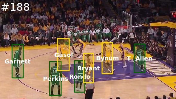
IEEE TRANSACTIONS ON PATTERN ANALYSIS AND MACHINE INTELLIGENCE 7
Algorithm 1 EM for weakly supervised learning data still remains unlabelled, i.e., there is no one-to-
1: estimate θ 0 by using labeled data xL and yL one mapping between yu and xu . Taking professional
2: k = 0 basketball games as an example, a team usually has 12
3: repeat players in their roster, and therefore |C| = 12. However,
4: k =k+1 in any given time t, there are only 5 players on the court,
5: ŷU = LinearProgramming(xU , θ k−1 ) . Eq. 11–15 and thus |Pt | = 5. In the experiments, we will show that
6: θ k = MultiLogitRegFit(yL , xL , ŷU , xU ) . Eq. 18 this play-by-play prior is crucial to train the identification
7: until convergence system with very small number of labeled training data.
8: return θ k
5 H OMOGRAPHY E STIMATION
Knowing the players’ locations on the court coordinates
We then compute the initial model parameters θ 0 by
is needed for many applications such as the automatic
maximizing the log-posterior with a L1 regularizer, as in
collection of player statistics. In order to achieve this,
Equation 16. Then, in the first iteration, we predict the
a transformation between the image and court coor-
identities of the unlabeled training data by solving the LP
dinates is required. Unfortunately, camera calibration
problem in Equation 11 with the initial parameters θ 0 .
algorithms [43], [44] are inapplicable due to the pan-tilt-
This is called the E-step because we compute the expected
zoom camera and the lack of an auxiliary plane in sports
value of yt,d given the current model. Then, we optimize
videos. We instead seek to compute the homography
the log-posterior with all training data:
transformation between the image and the court plane,
XX as in [45], [46], and [47].
max p(yu |xu , θ old ) [log p(yu |xu , θ)]
θ u∈U yu The relationship between a point p = [x, y]T in
X (17) the court coordinate and its corresponding point p0 =
+ log p(yl |xl , θ) − α||θ||1 [x0 , y 0 ]T in the image coordinate can be specified by:
l∈L
1 h1 x + h2 y + h3
where L is the set of labeled data, U is the set of p0 = = f (p; H) (20)
h7 x + h8 y + 1 h4 x + h5 y + h6
unlabelled data, and θ old are the parameters in the
previous iteration. We approximate the summation over where f (p; H) is a nonlinear function, and H = [h1 . . . h8 ]
yu by using the prediction ŷu generated from LP, i.e.: is the homography. In order to obtain the pairs of cor-
X X respondences (p, p0 ), the standard approach is to extract
max log p(ŷu |xu , θ)+ log p(yl |xl , θ)−α||θ||1 (18) and match interest points such as SIFT features [36] in
θ u∈U l∈L both images. However, in sports videos, most interest
points are generated from players and spectators, but
Specifically, for labeled data, we use the groundtruth
not from the court [47]. Using point correspondences
labels y provided by human annotators. For unlabelled
of players and spectators to estimate the homography
data, we use the predicted label ŷ computed in the E-
usually leads to unreliable results.
step. The optimization problem can be efficiently solved
To tackle this problem, we apply a model-based ap-
by [41]. This is called the M-step because we maximize the
proach inspired by [45]. Instead of matching interest
log-posterior given expected labels generated from the E-
points of two images, we match the court model with
step. We repeat this process until convergence to obtain
the edges of the video frames to establish correspon-
the best parameters. Since our semi-supervised learning
dences. As shown in Figure 6(d), we construct a court
algorithm is a coordinate ascent algorithm, it is guar-
model consisting of a point set M = [p1 . . . pn ], where
anteed to monotonically converge to a local maximum. T
Algorithm 1 summarizes the EM-based semi-supervised pi = [x, y] is a 2D point. Since all professional courts
learning algorithm. of the same sport have identical dimensions, this model
only has to be constructed once for a sport. The edges
In the standard semi-supervised learning, we set the
1 of the video frames are computed by the Canny detector
prior p(ŷt,d ) = |C| , where |C| is the number of all possible
[48], as shown in Figure 6(b). Since the edge detections
players. This means that the predicted label ŷt,d has a
contain many false responses from non-court objects,
uniform probability to be any of the |C| possible players.
we further utilize the detection results in section 3.1 to
When the play-by-play text is available, we set:
remove edges caused by players, as shown in Figure 6(c).
1 This article adopts a variant of the Iterated Closest
if c ∈ Pt Points (ICP) [49] to estimate the homography. Firstly,
p(ŷt,d = c) = |Pt | (19)
0 otherwise we manually specify the first-frame homography H1 and
transform the model such that M1 = H1 M (However, it
where Pt is a set of player that appears in frame t, and is possible to use a semi-automatic approach to initialize
Pt ⊂ C. We call this strategy weakly supervised learning the first-frame homography, as shown in [50]). Given the
because we are given additional constraints provided second frame, we use ICP to compute the frame-to-frame
by the play-by-play text. Notice that the majority of homography H12 . Specifically, for every model point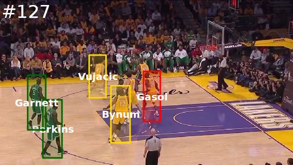
IEEE TRANSACTIONS ON PATTERN ANALYSIS AND MACHINE INTELLIGENCE                                                             8

                 (a) raw                          (b) original edge map                      (c) filtered edge map

            (d) model points                   (e) model and stable points               (f) homography estimation

Fig. 6. Estimating the homography in basketball videos. (a) A raw video frame. (b) Canny edges [48] of the frame. (c)
Filtered Canny edges by dropping edges caused by players. (d) The original model points. (e) The original model point
set augmented by stable points. (f) Homography estimation results by a variant of Iterated Closest Point (ICP) [49].

p ∈ M1 that appears in the first frame, we search for            position, and therefore we will have Et (p̃) = 1 for many
the closest edge point p0 in the second frame to establish       frames. Utilizing this fact, we maintain a score map St
the correspondence (p, p0 ). We drop correspondences             whose size is identical to Et , and update it according to:
with inconsistent edge normal directions to improve
                                                                                  St = αEt + (1 − α)St−1                (22)
the robustness, as suggested in [45]. The homography
is estimated by solving the following nonlinear least-           where 0 < α < 1 is a constant forgetting factor. A
square system [51]:                                              point is considered as stable if its score is higher than
                     X                        2                  a threshold. Figure 6(e) shows the original model points
                min       (f (pi ; H) − p0i )         (21)       and stable points of a professional basketball court. The
                 H     i
                                                                 stable points are automatically generated by Equation 22.
The optimization problem can be solved efficiently
by the Levenberg-Marquardt algorithm [38]. Then, we              6     R ESULTS
transform the model points by the new homography.                6.1   Data
We iterate the process of finding closest points and
least-square fitting until convergence to compute the fi-        We used videos from the 2010 NBA Championship series
nal frame-to-frame homography H12 . The second-frame             (Los Angeles Lakers vs. Boston Celtics). The original
homography can be thus derived by H2 = H12 H1 .                  videos consist of different kind of shots, and we only
Since camera motion is minor in two consecutive frames,          used the shots taken from the court view in this article.
ICP usually converges within 3-5 iterations. We repeat           The training set consists of 153160 detected bounding
this process for all subsequent frames in a video clip.          boxes across 21306 frames. The test set has 20 video
Figure 6(f) shows the homography estimation results,             clips, consisting of 13469 frames with 90001 detections.
where red lines represent the transformed basketball             The test clips varied in length, with the shortest at 300
model in a test video frame.                                     frames and longest at 1400 frames. They also varied in
   Sometimes, model points are sparse in video frames            level of identification difficulty. Labelling both training
due to the camera’s viewpoints or occlusions. To alle-           and test sets took us considerable effort (more than 300
viate this problem, we augment the model point set               hours). The size of this training data set is comparable
by stable points that have a consistent homography as            or larger than others in the weakly labeled learning liter-
the court plane. These stable points are usually marks           ature. For example, in previous work on high-resolution
or logos on the court, which vary in different stadi-            movies, [22] trained/tested on 49447 faces, and [20]
ums. Specifically, we construct an edge map Et where             trained on about 100000 faces.
Et (p̃) = 1, for p̃ = f −1 (p0 , Ht ) where f −1 (·) is the
inverse transformation that back-projects p0 in the image        6.2   Tracking evaluation
coordinate to the court coordinate. If a point p0 lies on        We use precision and recall to evaluate the performance
the court plane, it will be always projected to the same         of player detection, team classification, and multi-target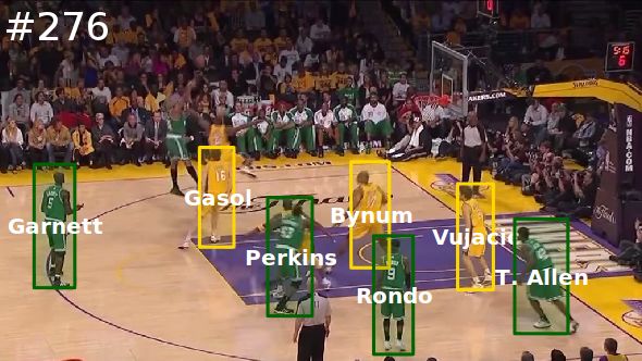
IEEE TRANSACTIONS ON PATTERN ANALYSIS AND MACHINE INTELLIGENCE                                                               9

tracking. The DPM detector [29] had a moderate preci-
sion 73% and recall 78% in the test basketball dataset.
DPM detected most players, but it also detected false
positives such as referees and spectators. After team
classification, the precision increases to 97% while it
retains a recall level of 74% in the basketball dataset. The
precision is significantly improved because we utilized
jersey colors to discard false positives generated from
referees and spectators, who wore clothes of different
colors. The tracking algorithm has a 98% precision with
an improved recall of 82% in the basketball dataset. This        Fig. 7. Precision and recall of the proposed KF+DPM and
is because the original detections are temporally sparse,        BPF [4] on the hockey dataset (blue: KF+DPM, red: BPF).
and tracking helps to bridge the temporal gap between
disjointed detections.                                             method      PR      RC      FA     MT      ML      IDS
                                                                   BPF [4]    65.5%   50.8%    2.3   16.0%   14.7%     37
   We compare the proposed tracking algorithm                      KF+DPM     91.8%   79.7%    0.6   56.3%   20.8%     27
(KF+DPM) with the Boosted Particle Filter (BPF) [4].
We use the same hockey dataset released by the authors                                    TABLE 1
[4], which consists of 1000 frames of a broadcast hockey          Tracking results of the proposed KF+DPM tracker and
game. Figure 7 shows the precision and recall of both             BPF [4] on the hockey dataset, using the metrics in [8].
the proposed algorithm and the BPF. The BPF has an
average precision of 65.5% and an average recall of
50.8% over the 1000 frame hockey video (red lines). On
the other hand, the proposed algorithm has a higher                Since these three visual cues complement each other,
average precision of 91.8% and a higher average recall           combining the RGB color histograms, MSER, and SIFT
of 79.7% (blue lines). We also compare the performance           yields the best results. For Lakers, the accuracy achieves
by using the metrics proposed in [8]. As shown in                85%, while in Celtics, the accuracy becomes 89%.
Table 1, we compare the tracking results of KF+DPM
and BPF by: Precision (PR), Recall (RC), False Alarm             6.3.2 Comparison of graphical models
(FA), Mostly Tracked (MT), Mostly Lost (ML), and ID              We then compare the effectiveness of the graphical
Switches (IDS). We can see that KF+DPM outperforms               model in Figure 9. Similar to the previous experiments,
BPF in all aspects except ML. This is partially due to           we randomly choose 30000 labeled image patches, and
a better detector (DPM) which has a better precision             then use the supervised learning to train the identifi-
and recall, and a more sophisticated motion model                cation system. The IID model assumes that there is no
(Equation 1) that is able to resolve ID switches.                connection between any identity nodes yt,d . In other
                                                                 words, we identify players by only the feature potential
                                                                 in Equation 2, but without using the temporal and
6.3   Identification evaluation
                                                                 mutual exclusion potentials. The identification results
The identification system achieves an average accuracy           are poor, having an accuracy about 50% for Lakers
of 85% for Lakers players and 89% for Celtics players.           and 55% for Celtics. This demonstrates the challenges
In addition, using weakly supervised learning greatly            of identifying players from a single-view camera. Since
reduces the number of labels required to train the iden-         players constantly change their poses and orientations, it
tification system (from 20000 to mere 200 labels for all         is very difficult to identify players from a single image.
players in a team). The following will provide a detailed           Adding temporal potentials to the model significantly
analysis.                                                        boosts the performance. In Lakers, the accuracy increases
                                                                 to 81%, while in Celtics, the accuracy increases to 85%.
6.3.1 Comparison of features                                     Temporal edges in the graphical model are constructed
We first compare the effectiveness of different features         by the tracking system. If the identification system has
in Figure 8. In the experiments, we randomly choose              high confidence about the identity of even a single image
30000 labeled image patches, and then use the super-             in a track (e.g., a frontal-view image of a player), this
vised learning approach in Equation 16 to train the              information can be passed forward and backward to the
identification system. Inference is performed by solving         entire track, and helps identify images of obscure views.
the linear programming problem in Equation 11–15.                   Adding mutual exclusion potentials to the model
  Among the three appearance features, the SIFT bag of           slightly improves the accuracy. In Lakers, the accuracy
words has the strongest discriminative power, followed           increases to 85%, while in Celtics, the accuracy becomes
by the MSER bag of words and RGB color histograms.               89%. Although the improvements are small, it is still
Colors are weak in this domain because players of                necessary to include mutual exclusion constraints in
the team wears uniforms of identical color, and many             order to prevent a duplicate of identities in a frame. In
players have very similar skin and hair colors.                  applications such as automatic collection of statistics and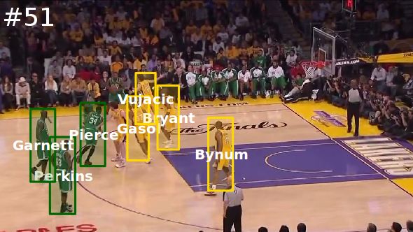
IEEE TRANSACTIONS ON PATTERN ANALYSIS AND MACHINE INTELLIGENCE                                                                     10

Fig. 8. Player identification results of different features              Fig. 9. Player identification results of different graphical
for Lakers (yellow) and Celtics (green). We compare the                  models for Lakers (yellow) and Celtics (green): feature
effectiveness of RGB color histograms, MSER bag of                       potentials only (IID), feature and mutex potentials (MU-
words [35], SIFT bag of words [36], and a combination                    TEX), feature and temporal potentials (TEMP), and the
of all features (ALL).                                                   full graphical model (FULL).

star-camera view, such duplications would significantly                     The weakly supervised approach also uses both labeled
reduce the quality, and thus they should be avoided.                     and unlabelled training data, and it also applies the EM-
                                                                         based algorithm (Algorithm 1). However, the weakly
6.3.3   Comparison of learning strategies                                supervised approach takes advantages of additional con-
Figure 10 compares different learning strategies for                     straints provided by the play-by-play texts, and it uses
player identification. In the training dataset, we perform               the prior in Equation 19. We can observe that weakly su-
supervised [2], semi-supervised, and weakly supervised                   pervised learning converges much faster than the semi-
learning, with different number of labeled training data.                supervised one, and it can achieve similar accuracies by
Then, we test the learnt classifiers in the testing dataset              using merely 200 labeled examples. This is a significant
while no labels (neither strong nor weak labels) are avail-              reduction of labeled training data, compared with 2000
able. Since some algorithms have random initialization,                  labels needed for semi-supervised learning, and 20000
we repeat the experiments for 10 times to compute the                    labels required for supervised learning.
mean and standard deviation.                                                For comparison, we also show results of ambiguous
   The supervised learning utilizes only labeled training                label learning [20]. Ambiguous label learning assumes
data yL and xL to train the model using Equation 16. We                  that every training image is associated with a set of
can observe that the identification accuracy in the testing              labels, one of which is the correct label for the image.
dataset converges slowly with the increase of labeled                    Since facial features in the original implementation of
training data3 . In both Celtics and Lakers, accuracies                  [20] are not suitable in this case, we replace them by the
converge after using more than 20000 labeled training                    proposed visual features. We train the classifier using
examples.                                                                all our training images, with corresponding label sets
   The semi-supervised approach uses both labeled train-                 provided by the play-by-play texts (the set size is 1 for
ing data yL and xL , and unlabelled training data yU                     labeled images and 5 for unlabelled images). After train-
and xU . This approach uses the EM-based algorithm                       ing, we use the same LP inference algorithm to identify
(Algorithm 1) to train the model parameters θ. Since                     players, instead of the IID approach used in [20]. We
play-by-play texts are not provided, we set the prior                    can see that ambiguous label learning performs better
to an uniform distribution over all possible players, i.e.,              than the proposed EM-based algorithm while using a
             1
p(ŷt,d ) = |C| . The accuracies of semi-supervised learning             very small amount of labeled data (10–30 labels, or 1–3
                                                                         labeled images per player). This is because ambiguous
converge faster than the supervised one. Using only 2000
                                                                         label learning has a more sophisticated mechanism to
labeled examples, semi-supervised learning can achieve
                                                                         deal with weakly labeled data. However, after giving 30–
similar identification accuracies as the supervised one.
                                                                         50 labels (3–5 labeled images per player) to initialize the
  3. Since no strong/weak labels are used during testing, the accuracy   model in EM, the proposed weakly supervised approach
will not achieve 100%.                                                   quickly outperforms the ambiguous label learning. This
IEEE TRANSACTIONS ON PATTERN ANALYSIS AND MACHINE INTELLIGENCE 11
(a) (b)
Fig. 10. Player identification results of different learning strategies. In both figures, we show identification results (mean
and standard deviation) of strongly supervised, semi-supervised, weakly supervised learning, and Cour et al. [20],
with different numbers of labeled training data. Notice that the x-axis is in log-scale. The strongly supervised approach
uses only labeled training data in Equation 16. The semi-supervised approach uses both labeled and unlabeled
1
data in Equation 17, but it uses an uniform prior over all possible players, i.e., p(ŷt,d ) = |C| . The weakly supervised
approach also uses both labeled and unlabeled data in Equation 17, but it uses the prior in Equation 19 provided by
the play-by-play texts. (a) Identification results for Celtics. (b) Identification results for Lakers.
is because the proposed EM algorithm utilizes the tem- transformed by the annotated homographies and points
poral and mutual exclusion potentials to help deal with transformed by the estimated homographies. We test on
ambiguous images (e.g., profile views), while the am- 5969 frames with annotated homography.
biguous label learning classifies every image indepen-
dently in the learning phase4 . The average error of homography is 7.32 pixels on
1280 × 720 images, or 13.65 cm on the basketball court
6.3.4 Comparison to the existing system [2]
(23.65m × 15.24m), which is very small. Figure 11(a)
Our previous work [2] reported a 85% identification shows the estimation errors of one selected test clip.
accuracy for Lakers and 82% identification accuracy for We can see that errors are usually below 10 pixels,
Celtics players. Evaluating on the same dataset, the except the region between 200-th to 400-th frame, which
proposed system improves the identification accuracy to have fast camera motion. Fast camera motions usually
87% for Lakers and 92% for Celtics. Since both systems happen during offensive-defensive changes, and they
use the same feature vectors, the boost is resulted from cause significant motion blur that reduces the chance of
a better inference algorithm introduced in section 4.3. detecting edges of the court.
In addition, the proposed system also applies weakly
supervised learning to greatly reduce the number of
labelled training data required from 20000 to 200. We compare our algorithm with [47] in their hockey
Figure 13 shows tracking and identification results on dataset of 1000 frames, as shown in Figure 11(b). [47]
a basketball video. We see that the proposed system is uses a combination of SIFT matching and area mini-
able to track and identify multiple basketball players mization to estimate the homography. Their method has
effectively. Please go to our website5 for more results. an average error of 20.21 pixels in the hockey video
(green line). In comparison, the average error of ICP is
only 13.35 pixels (blue line), which reduces the errors by
6.4 Homography evaluation
33%. Since the image resolution is 1920 × 980 pixels, the
We measure the performance of homography estima- error is about 1.4% of the image size, which is similar to
tion by computing the average distance between points the basketball case. This demonstrates that the proposed
algorithm is effective in different kinds of sports videos.
4. [20] used tracking to reduce the number of training data, but they
did not utilize temporal consistency in their learning algorithm. The speed of ICP is also much faster (2 seconds per
5. http://www.cs.ubc.ca/∼vailen/pami/ frame), while [47] runs in 60 seconds per frame.IEEE TRANSACTIONS ON PATTERN ANALYSIS AND MACHINE INTELLIGENCE 12
(a) basketball
(a) Bynum
(b) hockey
Fig. 11. Homography estimation results in (a) basketball,
and (b) hockey, compared to [47]. Errors are measured by
the average distance between points transformed by the (b) Vujacic
annotated and estimated homography.
Fig. 12. The spatial histograms (heatmaps) of basketball
players. Players offend in the left-hand side while defend
6.5 Automatic collection of player statistics in the right-hand side. In all images, lighter colors mean
Statistics are very important for analyzing the perfor- higher values in the histogram. (a) Bynum: a center whose
mance of sports players. However, these statistics are job is to attack the basket from a short distance. (b)
recorded by human annotators during the game, which Vujacic: a 3-point shooter whose job is to shoot from a
is a very expensive and tedious process. long distance.
With the proposed tracking, identification, and ho-
mography estimation systems, it is possible to automat-
ically generate player statistics from a single video. In
Figure 12, we show the spatial histogram (heatmap) of a
player’s trajectory in the court coordinates. The heatmap between video frames and the court, and identifies
is generated by tracking and identifying a specific player the players. The identification problem is formulated
over 5000 frames, and project their foot locations from as finding the maximum a posterior configuration in
the image to the court coordinates. Specifically, we di- a Conditional Random Field (CRF). The CRF combines
vide the court into grids of 1 × 1 meter. If the player three weak visual cues, and exploits both temporal and
stands on top of the grid, its histogram value will be mutual exclusion constraints. We also propose a Linear
increased by one. The heatmap represents the probability Programming Relaxation algorithm for predicting the
of a player being in each grid cell. best player identification in a video clip. For learn-
Since different players possess different motion pat- ing the identification system, we introduce the use of
terns and playing styles, the heatmap might be used to weakly supervised learning with the play-by-play texts.
identify players. We tried adding the heatmap as features Experiments show that the identification system can
to Equation 2, but we found that this had negligible achieve similar accuracies by using merely 200 labels in
effect on performance. One possible reason is that there weakly supervised learning, while a strongly supervised
are 12 players in a team, but only 3 distinctive playing approach needs a least 20000 labels.
styles and heatmaps. We anticipate that the heatmap
Note that the identification system relies on the track-
would work better to identify players in sports such like
ing system to construct the graphical model. When track-
soccer, where players have more diverse motion patterns
ing results are unreliable, one may consider enabling
and playing styles. Nevertheless, localizing players on
the weak interactions in Equation 4 (set > 0) in
the court is a useful output of the system, even if it does
order to split unreliable tracks [2], or adding another
not help with player identification.
weak interaction between the ends of two tracklets to
encourage merging [10]. In both cases, max-product or
7 D ISCUSSION sum-product BP can be used for the inference. Another
We introduce a novel system that tackles the challenging possibility is to improve tracking algorithm itself by
problem of tracking and identification of players in modelling the player’s motion in the court coordinates
broadcast sports videos taken from a single pan-tilt- instead of the image coordinates, as in [5]. This can be
zoom camera. The system possesses the ability to detect achieved by using the estimated homography to project
and track multiple players, estimates the homography players to the court coordinates.IEEE TRANSACTIONS ON PATTERN ANALYSIS AND MACHINE INTELLIGENCE 13
Fig. 13. Automatic tracking and identification results in a broadcast basketball video. Green boxes represent Celtics
players, and yellow boxes represent Lakers players. Text within boxes are identification results (player’s name), while
red boxes highlight misclassifications.
ACKNOWLEDGMENT [11] H. Jiang, S. Fels, and J. J. Little, “Optimizing Multiple Object
Tracking and Best Biew Video Synthesis,” IEEE Transactions on
This work has been supported by grants from the the Multimedia, vol. 10, no. 6, pp. 997–1012, 2008.
National Science and Engineering Research Council of [12] J. Liu, X. Tong, W. Li, T. Wang, Y. Zhang, and H. Wang, “Auto-
Canada, GEOIDE Network of Centres of Excellence, and matic player detection, labeling and tracking in broadcast soccer
video,” Pattern Recognition Letters, vol. 30, pp. 103–113, 2009.
the Canadian Institute for Advanced Research. We also [13] L. Ballan, M. Bertini, A. D. Bimbo, and W. Nunziati, “Soccer
thank for the National Basketball Association Entertain- players identification based on visual local features,” in CIVR,
ment for kindly providing us the image dataset. 2007.
[14] M. Bertini, A. D. Bimbo, and W. Nunziati, “Player Identification
in Soccer Videos,” in MIR, 2005.
R EFERENCES [15] M. Saric, H. Dujmic, V. Papic, and N. Rozic, “Player Number
Localization and Recognition in Soccer Video using HSV Color
[1] H. BenShitrit, J. Berclaz, F. Fleuret, and P. Fua, “Tracking Multiple Space and Internal Contours,” in ICSIP, 2008.
People under Global Appearance Constraints,” in ICCV, 2011. [16] Q. Ye, Q. Huang, S. Jiang, Y. Liu, and W. Gao, “Jersey number
[2] W.-L. Lu, J.-A. Ting, K. P. Murphy, and J. J. Little, “Identifying detection in sports video for athlete identification,” in SPIE, 2005.
Players in Broadcast Sports Videos using Conditional Random [17] X. Zhu and A. B. Goldberg, Introduction to Semi-Supervised Learn-
Fields,” in CVPR, 2011. ing. Morgan & Claypool, 2009.
[3] A. Yilmaz and O. Javed, “Object Tracking: A Survey,” ACM
[18] C. Vondrick, D. Ramanan, and D. Patterson, “Efficiently Scal-
Computing Surveys, vol. 38, no. 4, p. No. 13, 2006.
ing Up Video Annotation with Crowdsourced Marketplaces,” in
[4] K. Okuma, A. Taleghani, N. de Freitas, J. J. Little, and D. G. Lowe,
ECCV, 2010.
“A Boosted Particle Filter: Multitarget Detection and Tracking,”
[19] K. Barnard, P. Duygulu, D. Forsyth, N. de Freitas, D. M. Blei, and
in ECCV, 2004.
M. I. Jordan, “Matching Words and Pictures,” Journal of Machine
[5] Y. Cai, N. de Freitas, and J. J. Little, “Robust Visual Tracking for
Learning Research, vol. 3, pp. 1107–1135, 2003.
Multiple Targets,” in ECCV, 2006.
[6] D. Comaniciu, V. Ramesh, and P. Meer, “Kernel-Based Object [20] T. Cour, B. Sapp, C. Jordan, and B. Taskar, “Learning from
Tracking,” IEEE Transactions on Pattern Analysis and Machine In- Ambiguously Labeled Images,” in CVPR, 2009.
telligence, vol. 25, no. 5, pp. 564–575, 2003. [21] T. Cour, B. Sapp, A. Nagle, and B. Taskar, “Talking Pictures:
[7] M.-C. Hu, M.-H. Chang, J.-L. Wu, and L. Chi, “Robust Camera Temporal Grouping and Dialog-Supervised Person Recognition,”
Calibration and Player Tracking in Broadcast Basketball Video,” in CVPR, 2010.
IEEE Transactions on Multimedia, vol. 13, no. 2, pp. 266–279, 2011. [22] M. Everingham, J. Sivic, and A. Zisserman, “”Hello! My name
[8] B. Wu and R. Nevatia, “Detection and Tracking of Multiple, is... Buffy” - Automatic Naming of Characters in TV Video,” in
Partially Occluded Humans by Bayesian Combination of Edgelet BMVC, 2006.
based Part Detector,” International Journal of Computer Vision, [23] J. Sivic, M. Everingham, and A. Zisserman, “”Who are you” -
vol. 75, no. 2, pp. 247–266, 2007. Learning person specific classifiers from video,” in CVPR, 2009.
[9] B. Song, T.-Y. Jeng, E. Staudt, and A. K. Roy-Chowdhury, “A [24] O. Duchenne, I. Laptev, J. Sivic, F. Bach, and J. Ponce, “Automatic
Stochastic Graph Evolution Framework for Robust Multi-Target Annotation of Human Actions in Video,” in ICCV, 2009.
Tracking,” in ECCV, 2010. [25] I. Laptev, M. Marszalek, C. Schmid, and B. Rozenfeld, “Learning
[10] B. Yang, C. Huang, and R. Nevatia, “Learning Afnities and realistic human actions from movies,” in CVPR, 2008.
Dependencies for Multi-Target Tracking using a CRF Model,” in [26] M. Marszalek, I. Laptev, and C. Schmid, “Actions in Context,” in
CVPR, 2011. CVPR, 2009.You can also read