Traffic Prediction Framework for OpenStreetMap Using Deep Learning Based Complex Event Processing and Open Traffic Cameras - Schloss ...
←
→
Page content transcription
If your browser does not render page correctly, please read the page content below
Traffic Prediction Framework for OpenStreetMap
Using Deep Learning Based Complex Event
Processing and Open Traffic Cameras
Piyush Yadav1
Lero-SFI Irish Software Research Centre, Data Science Institute, National University of Ireland
Galway, Ireland
piyush.yadav@lero.ie

Dipto Sarkar
Department of Geography, University College Cork, Ireland
dipto.sarkar@ucc.ie

Dhaval Salwala
Insight Centre for Data Analytics, National University of Ireland Galway, Ireland

Edward Curry
Insight Centre for Data Analytics, National University of Ireland Galway, Ireland
edward.curry@insight-centre.org

       Abstract
Displaying near-real-time traffic information is a useful feature of digital navigation maps. However,
most commercial providers rely on privacy-compromising measures such as deriving location in-
formation from cellphones to estimate traffic. The lack of an open-source traffic estimation method
using open data platforms is a bottleneck for building sophisticated navigation services on top
of OpenStreetMap (OSM). We propose a deep learning-based Complex Event Processing (CEP)
method that relies on publicly available video camera streams for traffic estimation. The proposed
framework performs near-real-time object detection and objects property extraction across camera
clusters in parallel to derive multiple measures related to traffic with the results visualized on
OpenStreetMap. The estimation of object properties (e.g. vehicle speed, count, direction) provides
multidimensional data that can be leveraged to create metrics and visualization for congestion
beyond commonly used density-based measures. Our approach couples both flow and count measures
during interpolation by considering each vehicle as a sample point and their speed as weight. We
demonstrate multidimensional traffic metrics (e.g. flow rate, congestion estimation) over OSM by
processing 22 traffic cameras from London streets. The system achieves a near-real-time performance
of 1.42 seconds median latency and an average F-score of 0.80.

2012 ACM Subject Classification Information systems → Data streaming; Information systems →
Geographic information systems

Keywords and phrases Traffic Estimation, OpenStreetMap, Complex Event Processing, Traffic
Cameras, Video Processing, Deep Learning

Digital Object Identifier 10.4230/LIPIcs.GIScience.2021.I.17

Supplementary Material The system was implemented in Python 3 and is available at https:
//github.com/piyushy1/OSMTrafficEstimation.

Funding This work was supported by the Science Foundation Ireland grants SFI/13/RC/2094 and
SFI/12/RC/2289_P2.

1
    corresponding author
            © Piyush Yadav, Dipto Sarkar, Dhaval Salwala, and Edward Curry;
            licensed under Creative Commons License CC-BY
11th International Conference on Geographic Information Science (GIScience 2021) – Part I.
Editors: Krzysztof Janowicz and Judith A. Verstegen; Article No. 17; pp. 17:1–17:17
                   Leibniz International Proceedings in Informatics
                   Schloss Dagstuhl – Leibniz-Zentrum für Informatik, Dagstuhl Publishing, Germany
17:2   Traffic Prediction Framework for OSM Using Open Traffic Cameras

        1     Introduction

       OpenStreetMap (OSM) is arguably the largest crowdsourced geographic database. Currently,
       there are more than 5 million registered users, over 1 million of whom have contributed data
       by editing the map. Different aspects of OSM data quality have been scrutinized, and OSM
       data performed well on tests of volume, completeness, and accuracy across several classes
       of spatial data, such as roads and buildings [18, 11]. Despite standing up to data quality
       tests, enforcing data integrity rules required for a navigable road map is challenging. Lack of
       topological integrity and semantic rules such as turn restrictions which enable navigational
       capabilities is a stumbling block for OSM to be a viable open-source alternative to commercial
       products like Google Maps and Apple Maps.
           Over the last five years, several large corporations have realized the value of OSM and
       have assembled teams to contribute and improve data on the OSM platform [3]. Backed by
       large companies, the editing teams are capable of editing millions of kilometers (km) of road
       data each year. As a result of these efforts, the road network data on OSM is improving
       rapidly, and the gap in the quality of the data in the developed and developing countries
       is narrowing. In the foreseeable future, it is expected that widely available open-source
       navigation services may also be built on top of OSM data. The next frontier to making OSM
       more usable for navigational purposes is to have real-time traffic information to estimate trip
       times. This feature is already available in commercial digital navigation maps. However, the
       estimation and availability of traffic state data relies on platforms (i.e. iPhone and Android)
       built by the respective companies to feed data to the service.
           In recent years, internet-connected devices collectively referred to as the Internet of
       Things (IoT) have become ubiquitous. With the proliferation of visual sensors, there is
       now a significant shift in the data landscape. We are currently transitioning to an era of
       the Internet of Multimedia Things (IoMT) [2, 5] where media capturing sensors produce
       streaming data from different sources like CCTV cameras, smartphones and social media
       platforms. For example, cities like London, Beijing and New York have deployed thousands
       of CCTV cameras streaming hours of videos daily [1]. Complex Event Processing (CEP)
       is an event-driven paradigm which utilizes low-level data from sensor streams to gain high-
       level insights and event patterns. CEP applications can be found in areas as varied as
       environmental monitoring to stock market analysis [10].
           In this research, we propose a Complex Event Processing (CEP) framework to estimate
       traffic using deep learning techniques on publicly available street camera video streams. We
       process the data on GPU computing infrastructure and expose the processed output to OSM.
       The proposed method utilizes publicly available data and does not piggy-back on using cell
       phones. The solution is better for privacy and is also immune to subversion techniques such
       as the recent case where an artist used 99 Android phones to simulate traffic on Google
       Maps [12]. Further, the rich data stream from the video can provide multidimensional
       measurements of traffic state going beyond simple vehicle count-based metrics.

        2     Background and Related Work

       This section provides the initial background and techniques required for the development of
       a traffic estimation service for OSM.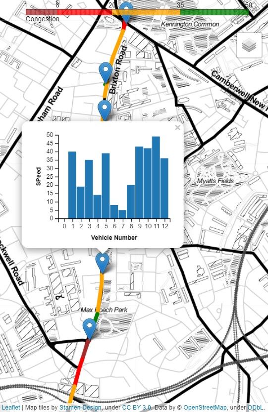
P. Yadav, D. Sarkar, D. Salwala, and E. Curry                                                                                                                                17:3

      Temperature Stream
                                                             Select FireWarningAlert(temp)
    55   52    49      52    47   41    41    40             from temp_sensor where avg.
                                                             (temp) > 50 °C within 5 mins                                              Fully Connected
  Avg.(temp) = 52 °C        Avg.(temp) = 42.25 °C
                                                         query                                                                               Layer
 t2=10                  t1=5                  t1=0
                                                                                                 Convolution     Convolution Pooling                     Car(1)
                                                                                                 and ReLU        and ReLU                                 Cat(0
                                   Receiver             Event
                                                                      Forwarder
                                                                                                               Pooling                                    ) Bus(0)
                                                       Matcher                    notification

                                        Event
                                       Operator                                                                                                                      Car
                                                    Complex Event Engine

    Figure 1 Complex Event Processing Paradigm.     Figure 2 CNN Architecture. A CNN con-
Temperature is being monitored from a sensor to sisting of several connected layers of neuron for
issue fire warnings.                            object identification from an image.

2.1           Complex Event Processing
Complex Event Processing (CEP) is a specialized information flow processing (IFP) technique
which detects patterns over incoming data streams [9]. CEP systems receive data from
different sensor streams and then mine high-level patterns in real-time to notify users. CEP
systems perform online and offline computations and can handle high volume and variety
of data. In CEP, event patterns of interest are expressed using SQL like query language,
and once a query is registered, it continuously monitors the data stream. Pattern matching
for queried patterns occurs in (near) real-time as the data flows from the Data Producers
(sensors) to the Consumers (applications).
    Fig. 1 shows a simple CEP system, where a user queries from a temperature sensor to
send notification of a fire warning alert if the average temperature is greater than 50°C in
the last five minutes [28]. The fire warning alert query is registered in the CEP engine
which continuously monitors the data from the temperature sensor. The CEP engine will
raise a fire warning alert at time t1 − t2 as the average temperature of incoming streams is
higher than 50°C in the last five minutes. Thus, a complex fire warning alert is generated by
averaging simple ‘temperature event’ from the sensor.

2.2           Deep Learning-based Image Understanding
The computer vision domain focuses on reasoning and identifying image content in terms
of high-level semantic concepts. These high-level concepts are termed as objects (e.g. car,
person) which act as building blocks in understanding and querying an image. There are
different object detection algorithms like SIFT [16], which classify and localize the objects
in the video frames. Convolutional Neural Networks (CNN) based deep learning methods
[15] are proficient at identifying objects with high accuracy. It is a supervised learning
technique where layers are trained using labelled datasets to classify images. Fig. 2 shows
the underlying architecture of a CNN model having different layers to classify and detect an
object from the image. CNN based object detection methods like YOLO [20] detect and
classify objects by drawing bounding boxes around them.

2.3           Related Work
Traffic Estimation Services. Most of the traffic monitoring related data is collected from
sensor devices like GPS embedded in mobile phones and speed detection cameras (loop
detectors, camera, infrared detectors, ultrasonic, radar detectors) [4]. The traffic data is
displayed on proprietary maps such as Google, Apple and Here Maps. These companies also
expose the data through APIs. However, the methodology for traffic estimation is opaque,

                                                                                                                                                                           GIScience 2021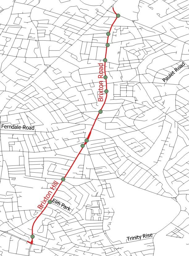
17:4   Traffic Prediction Framework for OSM Using Open Traffic Cameras

                                                                          Producer                              Consumer

                                                                                                          Identify Traffic
                                                          Camera 1                                  Query Congestion on Holloway
                                                                                       Complex            Road in every 1 minute
                                                                                     Event Engine
                                                                     Camera n                             Notification
                                                                                                                High Congestion
                                                                                                                   No Congestion
                                                                                                                        Low Congestion

            Figure 3 TfL Traffic Camera Dashboard.         Figure 4 Traffic CEP Overview.

       and depending on the service provider, there are costs and restrictions on how a third-party
       developer can utilize the data. Initiatives such as OpenTraffic2 are building an open-source
       data platform and services which collect anonymized telemetry data from vehicles and
       smartphones and exposes them through OSM API. OpenTraffic is a relatively new platform
       and is still building up a list of partners (currently three) to gather traffic information. Other
       attempts to create open traffic data framework for consumption as a map service include the
       OpenTransportMap3 project. Their framework is based on pre-calculated estimates of traffic
       volumes based on demographic data. There are some traffic state prediction works which
       use interpolation techniques using sensor-based reading like GPS and LIDAR to identify
       traffic at unknown locations [17, 31, 23]. In this work, instead of telemetry data like GPS,
       we focused on clusters of openly available video feeds which provide live-streaming updates
       from multiple locations and update traffic in real-time on OSM.

       Video-Based Traffic Estimation. Video streams are an ideal example of BigData as it
       represents a high volume, high velocity, unstructured source of data. Fatih et al. [19]
       proposed a Gaussian based Hidden Markov Model (GM-HMM) to estimate traffic over
       MPEG videos. But their work was limited only to the camera Field of View (FoV) to
       determine the traffic over a highway segment. In this work, we focused on estimating traffic
       beyond camera FoV across the whole queried street network even where camera feeds are not
       available. Kopsiaftis et al. [14] used background estimation over high-resolution satellite
       video images and performed traffic density estimation by counting vehicles in the given
       region. Again, their work is limited to only pre-recorded historical video data. On the
       other hand, our proposed framework estimates traffic over streaming video in near-real-time.
       Connected vehicles are another data source for traffic estimation. Kar et al. [13] proposed
       real-time traffic estimation considering vehicles as edge nodes. They performed object and
       lane detection using dash cameras installed in the vehicles to estimate their speed. The
       author’s future work was focused on sharing such data across vehicles and on a cloud-based
       map service. Our work builds upon this line of argument by considering traffic camera
       network as a cluster of edge nodes and then applying data-driven techniques to identify
       traffic across the road network which is later updated to OSM.

       2
           opentraffic.io
       3
           opentransportmap.info
P. Yadav, D. Sarkar, D. Salwala, and E. Curry 17:5
3 Motivation and Problem Scope
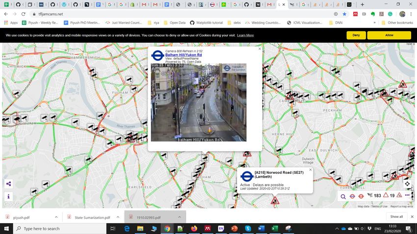
3.1 Case Study: London- A City of Open Traffic Cameras
London possesses an extensive camera network. The city is dotted with nearly 500K cameras
[26]. With a density of 68.4 cameras per 1000 people, it is estimated that an average Londoner
is caught in a camera approx 300 times a day [26]. Live camera feeds stream real-time
information of things happening around London’s streets, enabling applications like license
plate reading. The camera streams API is provided from Transport for London (TfL) and
can be accessed by registering with their system. Each video camera comes with metadata
including date, timestamp, street name and its geolocation. Availability of open cameras,
accessibility of real time4 and archived data5 , and friendly streaming API makes London
ideal for our case study. Fig. 3 shows the screenshot of camera networks across a part of the
city with a video clip instance from a particular camera.
3.2 User Scenario
Traditional traffic monitoring using CCTV is mostly a manual effort where traffic personnel
monitor the situation by looking at the feeds from cameras installed across the city. This
manual approach is time-consuming, tedious, and error-prone as it is difficult for humans to
synthesize a large number of events occurring across space and time. Thus, the development
of automated techniques is crucial to supplement manual qualitative efforts. Suppose the
traffic authority wants to map the busiest routes of the city over the day in real-time and
wants to provide the traffic state as a service to the citizens. Fig. 4 shows the authority using
a CEP engine to obtain the traffic congestion status over a road segment from a cluster of
CCTV cameras installed along the road. Processing this query over multiple video streams
requires identifying objects (e.g. cars), determining their properties (e.g. speed), calculating
traffic states, interpolation across the road network for continuous estimation, and visualizing
the results in real-time with summarized metrics and visualizations overlaid on OSM.
3.3 Multidimensional Traffic Analysis
There are multiple factors related to traffic and untangling the impact of individual factors
responsible for congestion is challenging. Congestion is a function of both: the physical
way vehicles (and other road users) interact with each other, and the people’s perception
of congestion (e.g. ‘the traffic is terrible today’) [24]. We focus on the primary factors
related to the physical dimensions of vehicular movement through the road network, namely
vehicle count and average vehicle speed. Thus, at each time point, we estimate the number
of vehicles at a location and the speed of each vehicle.
While these represent rudimentary aspects related to quantifying traffic state, they can be
used as building blocks to more complex metrics such as traffic density, expected travel time,
free flow ratio, and estimates of delay [24, 14]. No single indicator can be a ‘catch-all’ metric
to represent the problem. Reliance on a single parameter in describing network performance
paints an incomplete, or in some cases an incorrect picture of travel conditions. In this
paper, we focus on building the stream data processing architecture and show its efficacy
on a real-world application by focusing on calculating the basic metrics of vehicle count
and vehicle speed. Table 1 and Table 2 lists the macroscopic traffic metrics and Level of
Service(LOS) parameters [8] which are consider for evaluation in this work.
4
https://www.tfljamcams.net/
5
http://archive.tfljamcams.net/
GIScience 2021
17:6   Traffic Prediction Framework for OSM Using Open Traffic Cameras

         Table 1 Traffic Metrics.

                 Traffic Metrics                   Definition
                Traffic         Flow              TF is the total count of vehicles that have passed a certain
                (TF)                              point in both directions for a given time. TF is calculated
                                                  over short duration’s (e.g. two days) and then approx-
                                                  imated over days adjusting for seasonal and weekly vari-
                                                  ations. The TF can be calculated at different timescales
                                                  ranging from minutes, hours, daily, weekly and yearly
                                                  level (Annual Average Daily Traffic).
                Average Traffic                   It is the average speed of vehicles on both directions at
                Speed (ATS)                       a point for a given time scale. ATS is measured in m/s,
                                                  km/hr or mph.
                Traffic Density                   TD or volume (V) is the number of vehicles per unit
                (TD) and Capa-                    distance over a given road. It is measure in term of the
                city(c)                           number of vehicles per unit road (Km or mile). The
                                                  maximum number of vehicles in a mile per lane which a
                                                  road can accommodate is termed as capacity.

         Table 2 Level of Service.

                      Level of               Description                                        Volume-
                      Service                                                                   Capacity
                                                                                                Ratio
                                                                                                (V/C)
                      A                      Free flowing and highest driving                   1.0
                                             frustration.

                                      VIDEO STREAM MANAGER                          QUERY MANAGER

                           TT                         RMTP Media Server
                                  Video Stream

                                                                                                           Interface

                           ff
                                    Interface

                                                                                                             Query

                           LL                           Encoder Service            VEQL QUERY
                           AA                             (FFMPEG)                   ENGINE
                           PP
                           II                           Event Dispatcher

                                                                      Windows
                                                 YOLO Detector                        Vehicle Counter
                                                                                                                       O
                                                                                     Vehicle Speed and                 S
                                                                                     Direction Estimator               M
                                                                      State
                                                                     Manager         Traffic Congestion                A
                                 Deep Sort Object                                                                      P
                                                                                          Predictor
                                     Tracker
                                                                     Storage                                           I
                                                                                          Matcher
                          DNN MODELS INSTANCES                             COMPLEX EVENT ENGINE

         Figure 5 System Architecture Overview.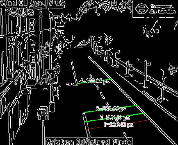
P. Yadav, D. Sarkar, D. Salwala, and E. Curry                                                        17:7

 4      System Architecture
To identify different traffic metrics using multiple cameras, a distributed microservice-based
complex event processing system is implemented. Fig. 5 shows the high-level architecture of
the traffic estimation system which is divided into four major components. These components
are independent microservices wrapped in a container and their instances can be deployed
over the cloud or local computing nodes. These components are:

     Query Manager: The user can subscribe to different queries using the query manager.
     The Query manager consists of a Query Interface where users can write queries in Video
     Event Query Language (VEQL) to detect traffic patterns [29]. VEQL is a SQL-like
     declarative language where rules and operators can be written to identify pattern over
     video streams. The VEQL Query Engine creates a query graph to represent patterns.
     Further details of VEQL can be found in [29]. A sample VEQL query for traffic congestion
     is as follows:
                Select Traffic_Congestion(Object) from Brixton Road
                WHERE Object = ‘Car’ OR Object = ‘Bus’
                WITHIN Time_Window = 5 sec WITH CONFIDENCE >40%

     In the above query, the user subscribed for Traffic Congestion for ‘Car and Bus’ over
     Brixton Road camera network with an update of every five-seconds. The traffic congestion
     operator will be discussed in detail in Section 6.
     Video Stream Manager: The video stream manager connects to multiple video feeds
     using a video stream interface which is a network adapter to provide the connection to
     different streaming API’s. The TfL (Transport for London) unified API is used to bring
     together video data from street cameras to our system. The Query Manager forwards the
     road information(e.g. Brixton Road) to the stream manager which later uses metadata
     information from the TfL API to fetch video streams from the corresponding road camera.
     For example, we pass different lat-long coordinates of Brixton Road (e.g. 51.4812,-0.11065)
     using OSM which is then passed to the TfL API (https://api.tfl.gov.uk/Place?
     lat=51.4812&lon=-0.11065&radius=100&type=JamCam) to search cameras. The search
     process continues and iterates until the end of the queried road segment. Similarly, each
     stream is sent in parallel to the media server using the GStreamer library. Finally, the
     Event Dispatcher sends the received video streams from different cameras to the DNN
     Model pipeline.
     Deep Neural Network (DNN) Models Pipelines: This is a computer vision pipeline
     which consists of deep learning-based object detector and object tracker. The object
     detector model receives the video frames from the event dispatcher as a feature map and
     extracts the vehicles in the form of bounding boxes. The object detector is integrated
     with a DNN based object tracker to track the identified vehicle for a given length of time.
     The specifics of the object detector and tracker are explained in detail in Section 5.1.
     Based on the number of cameras on the queried road, separate DNN model instances are
     created dynamically to process each camera feed in parallel. This is necessary to separate
     the tracking instances of each identified vehicles in each camera.
     Complex Event Engine: The Complex Event Engine is the core component which
     predicts traffic-related activities. Its sub-components are:
        Window and State Manager: Data streams (i.e. video feeds) are considered as an
        unbounded timestamped sequence of data [35]. CEP systems work on the concept of

                                                                                                   GIScience 2021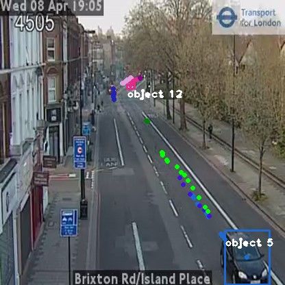
17:8   Traffic Prediction Framework for OSM Using Open Traffic Cameras

             state. Windows capture the stream state by taking the input stream and producing a
             sub-stream of finite length (equation (eq.) 1 and 2).
                 Svideo = ((f1 , t1 ), (f2 , t2 ), ......., (fn , tn ))                                 (1)

                 T IM E_W IN DOW (Svideo , t5sec ) : → S 0                                              (2)
                                                           0
             where fi are video frames and S = ((f1 , t1 ), (f2 , t2 ), ......., (fn , t5sec )). In eq. 2, a
             T IM E_W IN DOW of five seconds is applied over an incoming video stream Svideo
                                                        0
             (eq. 1) and gives a fixed sub-sequence S of five seconds of video data. The State
             Manager handles the created window state and sends the state information to the
             persistent storage and matcher services. The current work focuses on online processing
             of the data in near-real-time. The Storage component stores the event state of video
             feeds for historical batch-based analysis.
             Matcher: The Matcher performs traffic operations over the received state from the
             state manager. The matcher consists of three traffic-related operators 1) Vehicle
             Counter, 2) Vehicle Direction and Speed Estimator, and 3) Traffic Congestion Estima-
             tion. The functionality of these operators is explained in details in Section 5 and 6.
             The matcher finally sends the results of the CEP engine to the OSM layer through the
             OSM API.

        5     Computer Vision Pipelines for Traffic Classification
       Two computer vision pipelines have been developed for the CEP Engine to estimate the traffic
       service. The first pipeline performs object detection (e.g. cars, buses) and tracking over
       incoming video streams. The second pipeline involves calculation of traffic-related properties
       from objects (speed, direction and count) and interpolating traffic information from point
       sources to create a continuous surface over OSM.

       5.1    Pipeline 1: Vehicle Detection and Tracking
       Vehicle detection is a common problem in computer vision. Different object detection
       techniques ranging from feature-based matching like SIFT [16] and complex deep learning
       models have been used to identify vehicles in the videos. In this work, the YOLO v3 [20],
       a state-of-the-art object detection model is used for vehicle detection. The YOLO model
       considers object detection as a single regression problem and divides the image into a SxS
       grid to predict the objects bounding boxes and class probabilities simultaneously. The
       model gives real-time performance and processes 45 frames per second(fps) at the rate of
       22 milliseconds per frame on modern GPUs and is suitable for processing streaming data
       like videos. Five classes of vehicles- {bus, car, truck, bicycle and motorcycle} are selected
       as they represent the significant vehicular traffic on the road. We have used the YOLO
       model pre-trained on the COCO dataset which already consists of all the above five vehicular
       classes. The model outputs the bounding box coordinates of each detected vehicle with a
       probability score. The probability score is the model confidence to predict the class of an
       object (like vehicle), and experimentally we found that score greater than 0.4 detect most of
       the vehicles accurately.
           Videos are timestamped continuous sequence of image frames. The vehicle object detector
       process frames one-by-one to detect and classify vehicles per frame. Videos are temporally
       correlated where the same object (vehicles) remain in multiple frames. To avoid repeatedly
       counting the same vehicle, the vehicle needs to be tracked across the video feed. Deep-
P. Yadav, D. Sarkar, D. Salwala, and E. Curry                                                                 17:9

                                                             7.31 m
                                                                                      Direction: Incoming
                                                                                      Speed: 39 km/hr

   Figure 6 (L-R) a)TfL Camera Image at Brixton Road/Island Place, b)Edge Detection to Identify
Lanes, c) Distance Identification Using Google Earth Referencing , d) Object Identification, Tracking,
Direction and Speed Estimation.

SORT [27] is a multiobject tracking algorithm which uses Kalman filters and deep neural
network to track the detected objects across the image frames. We integrated the DeepSORT
tracking model with the YOLO object detection to uniquely identify each vehicle across
frames.

5.2    Pipeline 2: Vehicle Direction, Count and Speed Estimation
It is essential to know the movement direction of the vehicle to segregate traffic estimation
for different lanes. Direction estimation is challenging in TfL installed cameras as there is no
metadata information about the direction of placement of the cameras on the road. After
close inspection, we concluded that the cameras are placed over roads in such a way that their
FoV covers the length of the road (top-front view). The cameras are placed in South-North
or West-East direction such that outgoing traffic is in the left lane while incoming traffic is in
the right lane with respect to cameras FoV. The direction of each vehicle can be calculated
by measuring the displacement of the centre pixel location of its bounding box across frames
for a given time window (eq. 2). Considering the bottom left of the image frame as reference
origin, if the displacement of the y-axis value of centre point of bounding box decreases for a
given time, then it is considered an incoming traffic and vice-versa. DeepSORT provides each
vehicle with a unique id so that the counting can be done for vehicles in both directions.
     The speed of the vehicles can be identified using the standard equation of Distance =
Speed ∗ T ime. Thus, the displacement of the centre pixel point of vehicle across frames where
it is present for a given time (e.g. 5 sec) can be used to estimate the vehicle speed. But the
speed of the vehicle will be calculated in pixels/sec which is not helpful in traffic estimation.
As discussed earlier, there are no camera calibration points or pixel geotagging is available in
the metadata. In computer vision, object distance from the camera is measured by taking
pictures of the object from different angles and then fit into camera calibration equations. It
is infeasible to go to every camera points to get object pictures from different angles. We
performed a different approach to identify the relative pixels value in terms of metres. As
shown in Fig. 6(b), a canny edge detection [7] algorithm is used to identify the lanes of the
road using a background frame where no vehicles are present. The number of pixels between
two lanes is then calculated by dividing the image into two parts and taking average pixels
distance value between lanes to accommodate camera FoV at a different scale. Using the ruler
tool available in Google Earth, the distance between lanes is calculated for the same location
(figure 6(a,b,c)). For example, the number of pixels between lane is x and google earth distance
is y metres, then the size of each pixel is x/y metre. We used the Design Manual for Roads
and Bridges (DMRB) CD127 [25] document which provides highway cross-sections and traffic
lane width for trunk roads to validate that identified distance is within standard permissible

                                                                                                            GIScience 2021
17:10 Traffic Prediction Framework for OSM Using Open Traffic Cameras
v1 v0
1 v2
2
2
t0
Traffic Prediction
3
t1
4
v4
5
v5 t2
6
t3
3
7 vn-1
vn
8
Traffic Prediction
9
10
11
4
12
Figure 7 (L-R) a)OpenStreetMap portion of London, b)Brixton Road with Camera Points, c)
NB-IDW Technique Shown for Camera 2 and 3.
limits. Finally, for a camera cluster {c0 , c1 , c2 , c3 , · · ·} over a road, for each ci we process the
video streams to get information as: ci = {vehicleID : [class, direction, speed], · · ·} (figure
6(d)). This processed data is then used to identify traffic estimates across the street network.
6 Traffic Prediction Over Street Network
Traffic cameras are installed over the street at specified distances on important locations
like junctions and roundabouts. For example, in Brixton Road London the cameras are
placed at an average of 0.4 -0.7 km apart from each other. The traffic cameras have a
limited FoV extending over a few metres of the road. So, the proposed system will perform
vehicle detection and tracking within this camera FoV. There is no traffic-related information
available for a road segment located between the installed cameras. Thus, traffic interpolation
is required to identify the unknown traffic values along with street networks.
Algorithm 1 Traffic Congestion Estimation Operator Algorithm.
Data: CameraRoute ← {C0 , C1 , C2 , ..., Cn }
Result: Traffic Congestion Overlay on OSM
foreach (Ci , Ci+1 ) ∈ CameraRoute do
RShortestP ath ← getShortestP ath(Ci , Ci+1 );
T argetP oints ← identif yV ertices(RShortestP ath );
{O0 , O1 , O2 , ..., On } ← getObjectAndDirection(Ci , Ci+1 );
{S0 , S1 , S2 , ..., Sn } ← estimateObjectSpeed(Oi , O1 , ..., On );
SampleP oints ← {O0 , O1 , O2 , ..., On };
disnetwork ← getN etworkDistance(T argetP oints);
weightsspeed ← {S0 , S1 , S2 , ..., Sn };
traf f iccongestion ← doIDW (disnetwork , weightsspeed );
OSM ← displayCongestion(RShortestP ath , traf f iccongestion );
endP. Yadav, D. Sarkar, D. Salwala, and E. Curry 17:11
6.1 Network-based Traffic Interpolation
In GIS, interpolation is widely used in mapping terrain, temperature, and pollution levels.
Spatial interpolation is a prediction technique to estimate unknown values at different points
using values from sample locations. Common strategies for spatial interpolation assumes
that points are distributed over a 2D- Euclidean space and that the output is to be a surface
spanning the entire space. Measurement of distance between sample and target locations are
also done ‘as the crow flies’ along straight lines assuming that the space is isotropic and can be
traversed easily in every direction. These assumptions do not hold in the case of road networks
which are essentially 1D and can only be traversed along its length. Traditional spatial
interpolation approaches, when applied to network-based structures results in significant
errors. We performed a network-based Inverse Distance Weighted (NB-IDW) interpolation
method for traffic prediction over the road segment between installed cameras [21]. As
per Tobler’s Law which underpins spatial interpolation techniques, we model congestion by
assuming that nearby cameras that record high vehicle counts and low speed represent areas
of high traffic and assume an exponential distance decay function for interpolation.
Fig. 7(a) shows the Brixton Road instance in London over the OSM layer. The road
stretch is approximately 2.5 miles (Camberwell New Rd/Brixton Rd to Brixton Hill/Morrish
Rd) with 12 CCTV cameras (Fig. 7(b)) with an average density of 4.8 cameras per mile.
Fig. 7(c) shows the road segment between camera 2 and 4 and how the traffic values
were interpolated across this road section. Let {v0 , v1 , v2 , . . . , vn−1 , vn } be the identified
vehicles with speed {S0 , S1 , S2 , . . . , Sn−1 , Sn } in a specific direction for camera 2 and 3. Let
{t0 , t1 , t2 , . . . , tl−1 , tl } the target locations between camera 2 and 3 with unknown traffic
congestion values {cˆ0 , cˆ1 , cˆ2 , . . . , cn ˆ− 1, cˆn }. Therefore, the observed traffic congestion value
(cˆo ) is the weighted mean of the speed of nearby identified vehicles as:
n
X
cˆo = di Si (3)
i=1
In eq. 3 di is the network distance and Si is the speed of the vehicles from the target location.
The equation can be expanded as:
Pn
f (disnetwork (vi , t0 ))Si
Pi=1
n (4)
i=1 f (disnetwork (vi , t0 ))
In eq. 4, f (disnetwork (vi , t0 )) is the network distance between the vehicles sample points
and a given target location (t0 ). The road network is treated as a graph with nodes V and
edges E. The disnetwork is the shortest path distance between the vehicles and target point
and is calculated using Dijkstra algorithm while Haversine distance is used to calculate the
distance. In IDW, the weights are inversely proportional to the distance and are raised to
power value p (-ve for inverse relationship). With the increase in p, the weights of farther
points are decreased rapidly (eq. 5). Algorithm 1 details the traffic congestion operator and
the steps required to estimate the traffic.
Pn −p
i=1 (f (disnetwork (vi , t0 ))) Si
Pn −p (5)
i=1 (f (disnetwork (vi , t0 )))
The traffic congestion value will be higher if vehicles are nearer to the target points. For
example, in Fig. 7(c) traffic congestion value at the target point t0 will be more as compared
to t1 and t2 as number of vehicles (v0 , v1 , v2 ) near to t0 is greater. Now the question arises:
how many vehicles (such as v3 , v4 in Fig. 7(c)) are already present in the road segment?
GIScience 202117:12 Traffic Prediction Framework for OSM Using Open Traffic Cameras
The OSM layer for London provides the maximum speed (Smax ) of the road (48 mph), so
the maximum travel time between camera points can be derived. The speed of the vehicles
will lie in the range of 0 ≤ Si ≤ Smax . Suppose the camera feeds refresh every tcam−ref resh
seconds, then the distance covered by vehicle(vi ) will be:
Di = Si × tcam−ref resh (6)
Processing the camera video feeds are computationally intensive and leads to latency.
The given time needs to be added to the current time to know the location of the vehicle.
So, the total distance covered by the vehicle will be:
Di = Si × (tCam−ref resh + processing − latency) (7)
If the vehicle(vi ) covers the distance Di such that 0 ≤ Di ≤ maxroad−length where
maxroad−length is the distance between two cameras, then this vehicle will be considered as
sample points for traffic calculation. For example, let the distance between camera 2 and 3 is
1 mile (for easier calculation) and vehicle v0 at camera 2 is moving with speed(Si ) of 40mph
which is less than Smax (48mph). Suppose the camera feed refreshes (tcam−ref resh ) every
10 seconds and requires 2 seconds to process (processing − latency) the new video feed. In
such time the v0 will cover distance(Di ) = (40/3600)*(10+2) i.e. 0.13 mile and will be near
point t0 , t1 . Thus, we consider the vehicles which are identified from both the cameras and
the vehicles which are present in the road segments identified from previous feeds to perform
the an appropriate traffic calculation.
7 Experimental Results
7.1 Dataset and Implementation Details
Traffic Camera Data. For the experiments, two trunk roads (Brixton and Kennington)
were selected from the Lambeth borough of London. As mentioned in Section 4, the traffic
camera data feed was obtained from the TfL API by passing the camera location and search
radius. Table 3 shows the list of cameras (total 22) installed on selected roads. A total
3080 video clips with 140 video clips (9 seconds) per camera are processed to identify the
traffic status.
Hardware and Software. The system6 was implemented in Python 3 over the VidCEP
engine [29] running on a 16 core Linux Machine with 3.1 GHz processor, 32 GB RAM and
Nvidia Titan Xp GPU. The microservices were wrapped in Docker containers with Redis
Stream acting as a messaging service among the containers. The OpenCV library was used
for image processing and Darknet and PyTorch 7 deep learning framework were used for object
detection and tracking. GStreamer was used to stream camera video feeds from the TfL API.
OSMNX library fetched road network from OSM and calculated network distance [6].
Creation and Updating of Traffic Overlay over OSM. We used the Leaflet8 JavaScript
library to overlay traffic information over OSM. The Node.js server supporting the Leaflet
application was connected to the back-end system via Redis Streams. The Leaflet ColorLine
class was used to highlight the roads with the given colour intensity.
6
https://github.com/piyushy1/OSMTrafficEstimation
7
https://pytorch.org/
8
https://leafletjs.com/index.htmlP. Yadav, D. Sarkar, D. Salwala, and E. Curry 17:13
Table 3 List of Traffic Cameras for Study.
No. Brixton Road Cameras Kennington Road Cameras
C1 Camberwell New Rd/Brixton Rd Kennington Lane/Newington Butts
C2 Brixton Rd/Island Place Kennington Pk Rd/Penton Pl
C3 A23 Brixton Rd/Vassell Rd Kennington Pk Rd/Braganza St
C4 A23 Brixton Rd/Hillyard St Kennington Pk Rd/Kennington Rd
C5 A23 Brixton Rd/Ingleton St Kenington Pk Rd/Kennington Oval
C6 A23 Brixton Rd/Wynne Rd A3 Clapham Rd/Elias Place
C7 Brixton Rd/Stockwell Pk A3 Clapham Rd/Handforth Street
C8 Acre Lane/Coldharbour Lane A3 Clapham Rd/Crewdson Rd
C9 A23 Brixton Hill/Effra Rd A3 Clapham Rd/Caldwell St
C10 Brixton Hill /Lambert Rd A3 Clapham Rd/Landsdowne Way
C11 Brixton Hill / Elm Park A3 Clapham Rd/
C12 Brixton Hill/Morrish Rd NA
Figure 8 Traffic Congestion and Vehicle Speed Information over OSM.
7.2 Empirical Evaluation
Traffic Congestion Visualization over OSM. The traffic congestion is the interpolated
value superimposed over the road segment between the cameras. As discussed in Section
6.1, the number of vehicles, their direction (left or right lane) and speed is calculated. The
congestion is estimated for the road segment between the two cameras using e.q 5. The value
of p =2 is used as the distance decay factor for interpolation. The TfL API upload the video
feeds of 9 seconds (approx. 280 frames), and thus we process them in two TIME WINDOW
of 4.5 seconds (140 frames) each. Using eq. 7, for the second time window, we also estimate
if any vehicle from the previous window is present on the road segment and take this into
consideration for congestion.
Different map services calculate traffic congestion values, but they remain opaque about
their method. For example, Here Maps API provides Jam factor values and divides them
into four jam categories without explaining how the values are calculated. In this work,
count and speed are considered as parameters for congestion estimation; so if the speed of
vehicles is high then the traffic is considered smooth. As per OSM data, the maximum speed
GIScience 202117:14 Traffic Prediction Framework for OSM Using Open Traffic Cameras
Traffic Mean Speed(km/hr)
Traffic Flow per Hour
Average Latency (sec.)
Avg. F-Score
Pre-processing
Latency
(a) Brixton Road Traffic Camera Statistics Traffic Operator Latency System Latency
(c) Processing Latency
Traffic Mean Speed(km/hr)
Traffic Flow per Hour
Avg. F-Score
Road Length Capacity V/C LOS
(miles)
Brixton 2.5 2250 0.31 A
Kenning 1.4 1260 0.35 A
ton
(b) Kennington Road Traffic Camera Statistics (d) Vehicle to Capacity Ratio
Figure 9 Different Traffic Statistics for Roads Calculated Using Camera Video Feeds.
limit for the selected roads is 48mph (approx. 77km/hr). In Fig. 8, a four-step colour-based
traffic congestion over Brixton Road is shown where- 1)Green - No traffic (45-70 km/hr) 2)
Orange - light traffic (30-45 km/hr), 3)Red - moderate traffic(20-30 km/hr) and 4) Brown-
high traffic(10-20 km/hr). The above-defined congestion parameters range is not static and
can be reconfigured depending on requirements. Fig. 8(right) also shows specific traffic
data available by clicking anywhere along the road. Since we could not perform a direct
comparison with other map services, we can only visually compare that the traffic dynamics
they provide are similar to our proposed technique.
Traffic Flow Rate and Speed. As per Table 1, the Traffic Flow rate (TF) is the number of
vehicles in each lane per unit of time. TF is calculated for small periods and then extrapolated
to larger time scales. For example, if 20 vehicles observed in 10 minutes, then TF will be 120
vehicles per hour [22]. Fig. 9(a) and (b) shows the hourly TF for Brixton and Kennington
roads for both lanes. The camera C5 (Brixton-left lane) and C9 (Kennington-left lane) have
max. flow rate of 410 and 572 vehicles per hour. The reason behind such a low flow rate is
the lockdown measures currently in place in London because of the COVID-19 pandemic
situation. Fig. 9(a) and (b) shows the Traffic Mean Speed (TMS) which is the average speed
of vehicles recorded at a given point for a selected period. The Brixton road TMS ranges
between 18-46 km/hr while that of Kennington is from 20-58 km/hr. Cameras where speed
is below 20 km/hr is due to the video feeds having more red light signals. Fig. 8 shows the
TMS example on the OSM map where markers can be clicked to get the current traffic status
(e.g vehicle speed and count).
Traffic Density and Volume to Capacity Ratio(V/C). Traffic density is the number of
vehicles occupying a unit length of road. The Road Task Force from TfL specifies the capacity
of the road as 900 vehicles per mile. Fig. 9(d) shows the V/C ratio for both roads to identify
the Level of Service (LOS). During the experimentation time, the V/C ratio for Brixton and
Kennington was 0.31 (LOS-A) and 0.35 (LOS-A) respectively. As discussed earlier the lower
V/C ratio is due to lockdown measures as a result of COVID-19 restrictions.
Traffic Prediction Accuracy and Latency. The above-discussed traffic estimates are linked
to the performance of the object detector (YOLO) and tracker (DeepSORT) models. The
error in these models will directly propagate to the traffic estimates and skew the overallP. Yadav, D. Sarkar, D. Salwala, and E. Curry 17:15
results. F-score is the standard metric to identify the performance of the classifier. It is the
harmonic mean of precision and recall and is calculated as:
2 ∗ (P recision ∗ Recall)
F = (8)
P recision + Recall
In eq. 8, the precision is the ratio of relevant events matched and matched events while
recall is the ratio of relevant events matched
Pand
n
relevant events. The mean F-score of each
i=1 Fci
road camera (ci ) is calculated as Fmean = . A sample of 110 video clips (each of 9
n
seconds) from 22 camera clusters were taken to identify the F-score. Fig. 9(a,b) shows that
the mean F-score of the Brixton and Kennington camera is 0.78 and 0.80 respectively. The
error estimation rate which propagates can be calculated as ER = (actual-approx)/actual*100
and is 22% and 20% respectively for both roads camera clusters. The low F-scores for some
cameras were due to blurred FoV (like Kennington C1), tree shadows (like Kennington C1)
and faulty cameras (e.g. Brixton C9 which was not included).
Latency measures the time required by the framework to process the traffic information
and update it on the OSM. The latency can be divided into two stages: 1) Pre-processing
Latency- the time required by DNN models to process the video stream to track and extract
objects and 2) Traffic Operator Latency- the time required to compute traffic statistics from
pre-processed data and update it on the OSM. Fig. 9(c) shows the box plot of pre-processing
and traffic and system median latency of 0.071 seconds, 1.36 and 1.42 seconds, respectively
which implies a near-real-time performance.
8 Discussion of Limitations
While using camera feeds for traffic estimation poses privacy risks, the cameras are state
infrastructure with publicly available video streams. Open-source software built on top
of the open data infrastructure is more transparent compared to the opaque black-boxes
and data sources which certain corporations have exclusive access. As the quality of OSM
data improves, providing value-added services such as traffic estimation is essential for the
adoption of OSM as a mainstream routing service.
The uniqueness of this work lies in the query-based approach (VEQL) where users can
query multiple video streams by deploying operators (e.g. traffic congestion, flow rate, speed,
etc.) to the system. The framework can be deployed over the cloud and can be exposed
as an API to provide services over OSM. More complex and potential traffic services like
Vehicle Overtake and Lane Change [30] can be queried by creating operators and deploying
them to the system. Our method relies on existing cameras installed along road networks
and most of the limitations arise from camera deployment. For example, some cameras have
sub-optimal FoVs because of obstacles. Cameras in London have a relatively low refresh rate,
in the order of several minutes and provides only 9-second clips in each refresh cycle. Most
of the CCTV’s are installed in well-lit areas so the system can work in the night. Further,
incremental weather may result in object mismatch due to lack of training datasets in such
conditions. The inability to detect vehicles result in errors that propagate to final traffic
computation. We have tested our model on cameras placed over straight roads and the
strategy can be generalized for branched road networks.
In terms of generating visualizations for display over maps, it is possible to use more
complex spatial interpolation (e.g. kriging) and classification techniques to get better
congestion estimates. Using all cameras in a city will significantly improve the sample size
and provide better performance in the interpolation step leading to more accurate estimates of
travel time. The various measures of traffic we offer can also be used to create comprehensive
GIScience 202117:16 Traffic Prediction Framework for OSM Using Open Traffic Cameras
dashboards for communicating multi-dimensional aspects of traffic state. Finally, other open
data streams (e.g. General Transit Feed Specification) can also be integrated to supplement
traffic state calculations and estimation of travel times using different transport modes.
9 Conclusion
We have presented a traffic estimation framework built on open video streams based on open-
source deep learning technology. We have exposed the results and data through visualizations
on OSM. Exploiting the data from the video streams enabled us to extract traffic-related
parameters beyond simple vehicle counts. Combining these multiple parameters provides
opportunities to present a multidimensional analysis of the traffic state. For example, during
interpolation, we treated each vehicle as a sample point and its speed as weight, thus factoring
in both vehicle density and flow in the estimation of traffic. Users can utilize these parameters
to calculate their own metrics for congestion. The VEQL query empower users to create
their rules and deploy them as services for traffic-related events. We aim to deploy this
service across multiple cities which make their traffic camera feeds available to be able to
provide a comprehensive traffic state estimation service over OSM. We hope that places that
do not make their feeds available publicly will adopt our open-source framework to provide
their traffic estimation API to be consumed over OSM. Widespread adoption will provide
the currently lacking feature of traffic state information on OSM and will be a step towards
making OSM a viable alternative to commercial digital map service providers.
References
1 David Alm. Somebody’s Watching You: Ai Weiwei’s New York Installation Explores Surveil-
lance in 2017, 2017. URL: https://bit.ly/2Um1hT5.
2 Sheeraz A Alvi, Bilal Afzal, Ghalib A Shah, Luigi Atzori, and Waqar Mahmood. Internet of
multimedia things: Vision and challenges. Ad Hoc Networks, 33:87–111, 2015.
3 Jennings Anderson, Dipto Sarkar, and Leysia Palen. Corporate editors in the evolving
landscape of openstreetmap. ISPRS International Journal of Geo-Information, 8(5):232, 2019.
4 Waadt Andreas, Wang Shangbo, Jung Peter, et al. Traffic congestion estimation service
exploiting mobile assisted positioning schemes in gsm networks. Procedia Earth and Planetary
Science, 1(1):1385–1392, 2009.
5 Asra Aslam and Edward Curry. Towards a generalized approach for deep neural network
based event processing for the internet of multimedia things. IEEE Access, 6:25573–25587,
2018.
6 Geoff Boeing. Osmnx: New methods for acquiring, constructing, analyzing, and visualizing
complex street networks. Computers, Environment and Urban Systems, 65:126–139, 2017.
7 John Canny. An algorithm to estimate mean traffic speed using uncalibrated cameras. IEEE
Transactions on Pattern Analysis and Machine Intelligence, 8(6):679–698, 1986.
8 Thurston Regional Planning Council. Appendix o level of service standard and measurements.
URL: https://bit.ly/2z6yvzY.
9 Gianpaolo Cugola and Alessandro Margara. Processing flows of information: From data stream
to complex event processing. ACM Computing Surveys (CSUR), 44(3):15, 2012.
10 Alan Demers, Johannes Gehrke, Mingsheng Hong, Mirek Riedewald, and Walker White.
Towards expressive publish/subscribe systems. In International Conference on Extending
Database Technology, pages 627–644. Springer, 2006.
11 Mordechai Haklay. How good is volunteered geographical information? a comparative study
of openstreetmap and ordnance survey datasets. Environment and planning B: Planning and
design, 37(4):682–703, 2010.
12 Alex Hern. Berlin artist uses 99 phones to trick google into traffic jam alert, 2020. URL:
https://bit.ly/34ISrF4.P. Yadav, D. Sarkar, D. Salwala, and E. Curry 17:17
13 Gorkem Kar, Shubham Jain, Marco Gruteser, Fan Bai, and Ramesh Govindan. Real-time
traffic estimation at vehicular edge nodes. In Proceedings of the Second ACM/IEEE Symposium
on Edge Computing, pages 1–13, 2017.
14 George Kopsiaftis and Konstantinos Karantzalos. Vehicle detection and traffic density monit-
oring from very high resolution satellite video data. In 2015 IEEE International Geoscience
and Remote Sensing Symposium (IGARSS), pages 1881–1884. IEEE, 2015.
15 Yann LeCun, Yoshua Bengio, and Geoffrey Hinton. Deep learning. nature, 521(7553):436–444,
2015.
16 David G Lowe et al. Object recognition from local scale-invariant features. In iccv, volume 99,
pages 1150–1157, 1999.
17 Michael Lowry. Spatial interpolation of traffic counts based on origin–destination centrality.
Journal of Transport Geography, 36:98–105, 2014.
18 Pascal Neis, Dennis Zielstra, and Alexander Zipf. The street network evolution of crowdsourced
maps: Openstreetmap in germany 2007–2011. Future Internet, 4(1):1–21, 2012.
19 Fatih Porikli and Xiaokun Li. Traffic congestion estimation using hmm models without vehicle
tracking. In IEEE Intelligent Vehicles Symposium, 2004, pages 188–193. IEEE, 2004.
20 Joseph Redmon, Santosh Divvala, Ross Girshick, and Ali Farhadi. You only look once: Unified,
real-time object detection. In Proceedings of the IEEE conference on computer vision and
pattern recognition, pages 779–788, 2016.
21 Narushige Shiode and Shino Shiode. Street-level spatial interpolation using network-based
idw and ordinary kriging. Transactions in GIS, 15(4):457–477, 2011.
22 NCSU Transport Tutorial Site. Traffic flow fundamentals: Flow, speed and density. URL:
https://lost-contact.mit.edu/afs/eos.ncsu.edu/info/ce400_info/www2/flow1.html.
23 Yongze Song, Xiangyu Wang, Graeme Wright, Dominique Thatcher, Peng Wu, and Pascal
Felix. Traffic volume prediction with segment-based regression kriging and its implementation
in assessing the impact of heavy vehicles. Ieee transactions on intelligent transportation
systems, 20(1):232–243, 2018.
24 Burkhard Stiller, Thomas Bocek, Fabio Hecht, Guilherme Machado, Peter Racz, and Martin
Waldburger. Understanding and Managing Congestion For Transport for London. Tech-
nical report, Integrated Transport Planning Ltd., 2017. URL: http://content.tfl.gov.uk/
understanding-and-managing-congestion-in-london.pdf.
25 Unkown. Design manual for roads and bridges- cd 127 cross-sections and headrooms. Technical
report, Department for Transport UK, 2020. URL: https://www.standardsforhighways.co.
uk/ha/standards/.
26 Website. How many cctv cameras in london? URL: caughtoncamera.net/news/
how-many-cctv-cameras-in-london/.
27 Nicolai Wojke, Alex Bewley, and Dietrich Paulus. Simple online and realtime tracking with a
deep association metric. In 2017 IEEE international conference on image processing (ICIP),
pages 3645–3649. IEEE, 2017.
28 Piyush Yadav and Edward Curry. Vekg: Video event knowledge graph to represent video
streams for complex event pattern matching. In 2019 First International Conference on Graph
Computing (GC), pages 13–20. IEEE, 2019.
29 Piyush Yadav and Edward Curry. Vidcep: Complex event processing framework to detect
spatiotemporal patterns in video streams. In 2019 IEEE International Conference on Big
Data (Big Data), pages 2513–2522. IEEE, 2019.
30 Piyush Yadav, Dibya Prakash Das, and Edward Curry. State summarization of video streams for
spatiotemporal query matching in complex event processing. In 2019 18th IEEE International
Conference On Machine Learning And Applications (ICMLA), pages 81–88. IEEE, 2019.
31 Haixiang Zou, Yang Yue, Qingquan Li, and Anthony GO Yeh. An improved distance metric
for the interpolation of link-based traffic data using kriging: a case study of a large-scale urban
road network. International Journal of Geographical Information Science, 26(4):667–689, 2012.
GIScience 2021You can also read