Less is More: Robust and Novel Features for Malicious Domain Detection
←
→
Page content transcription
If your browser does not render page correctly, please read the page content below
Less is More: Robust and Novel Features for
                                                     Malicious Domain Detection

                                                   Chen Hajaj1 , Nitay Hason2 , Nissim Harel3 , and Amit Dvir4
                                         1
                                             Ariel Cyber Innovation Center, Data Science and Artificial Intelligence Research
                                                           Center, IEM Department, Ariel University, Israel
                                                                        chenha@ariel.ac.il
arXiv:2006.01449v1 [cs.CR] 2 Jun 2020

                                                             https://www.ariel.ac.il/wp/chen-hajaj/
                                               2
                                                 Ariel Cyber Innovation Center, CS Department, Ariel University, Israel
                                                                        nitay.has@gmail.com
                                                        3
                                                          CS Department, Holon Institute of Technology, Israel
                                                                         nissimh@hit.ac.il
                                               4
                                                 Ariel Cyber Innovation Center, CS Department, Ariel University, Israel
                                                                        amitdv@ariel.ac.il
                                                                https://www.ariel.ac.il/wp/amitd/

                                                Abstract. Malicious domains are increasingly common and pose a se-
                                                vere cybersecurity threat. Specifically, many types of current cyber at-
                                                tacks use URLs for attack communications (e.g., C&C, phishing, and
                                                spear-phishing). Despite the continuous progress in detecting these at-
                                                tacks, many alarming problems remain open, such as the weak spots of
                                                the defense mechanisms. Since machine learning has become one of the
                                                most prominent methods of malware detection, A robust feature selec-
                                                tion mechanism is proposed that results in malicious domain detection
                                                models that are resistant to evasion attacks. This mechanism exhibits
                                                high performance based on empirical data. This paper makes two main
                                                contributions: First, it provides an analysis of robust feature selection
                                                based on widely used features in the literature. Note that even though
                                                the feature set dimensional space is reduced by half (from nine to four
                                                features), the performance of the classifier is still improved (an increase
                                                in the model’s F1-score from 92.92% to 95.81%). Second, it introduces
                                                novel features that are robust to the adversary’s manipulation. Based
                                                on extensive evaluation of the different feature sets and commonly used
                                                classification models this paper show that models which are based on
                                                robust features are resistant to malicious perturbations, and at the same
                                                time useful for classifying non-manipulated data.

                                                Keywords: URL, Malicious, ML

                                        1     Introduction

                                        In the past two decades, cybersecurity attacks have become a major issue for
                                        governments and civilians [57]. Many of these attacks are based on malicious web
                                        domains or URLs (See Figure 1 for the structure of a URL). These domains are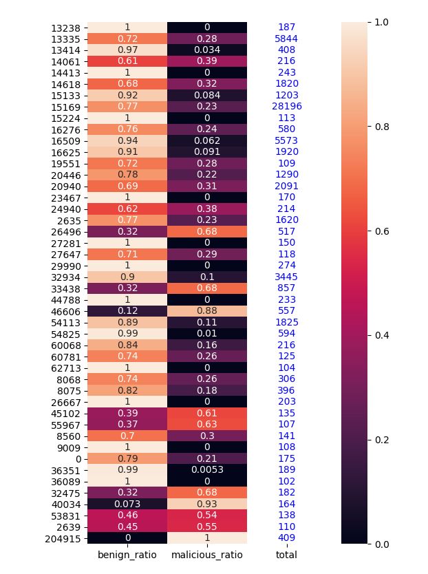
used for phishing [16,29,31,47,55] (e.g. spear phishing), Command and Control
(C&C) [53] and a vast set of virus and malware [19] attacks.

                             Fig. 1: The URL structure

    The Domain Name System (DNS) maps human-readable domain names to
their associated IP addresses (e.g., google.com to 172.217.16.174). However, DNS
services are abused in different ways in order to conduct various attacks. In such
attacks, the adversary can utilize a set of domains and IP addresses to orchestrate
sophisticated attacks [56,12]. Therefore, the ability to identify a malicious do-
main in advance is a massive game-changer [11,12,14,15,18,20,22,25,26,27,37,45,49,56,60,61,64].
    A common way of identifying malicious/compromised domains is to collect
information about the domain names (alphanumeric characters) and network in-
formation (such as DNS and passive DNS data1 ). This information is then used
for extracting a set of features, according to which machine learning (ML) algo-
rithms, are trained based on a desirably massive amount of data [12,13,14,15,18,20,25,26,27,37,45,46,49,60,64].
    A mathematical approach can also be used in a variety of ways [22,64], such
as measuring the distance between a known malicious domain name and the
analyzed domain (benign or malicious) [64]. Still, while ML-based solutions are
widely used, many of them are not robust; an attacker can easily bypass these
models with minimal feature perturbations (e.g., change the length of the domain
or modify network parameters such as Time To Live, TTL) [43,3].
    In this context, one of the main questions is how to identify malicious/compromised
domains in the presence of an intelligent adversary that can manipulate domain
properties.
    For these reasons, a feature selection mechanism which is robust to adversar-
ial manipulations is used to tackle the problem of identifying malicious domains.
Thus, even if the attacker has a black-box access to the model, tampering with
the domain properties or network parameters will have a negligible effect on the
model’s accuracy. In order to achieve this goal, a broad set of both malicious and
benign URLs were collected and surveyed for commonly used features. These fea-
tures were then manipulated to show that some of them, although widely used,
are only slightly robust or not robust at all. Thus, novel features were engineered
to enhance the robustness of the models. While these novel features support the
detection of malicious domains from new angles (e.g. autonomous system num-
bers), the resulting accuracy of models that were solely based on these features
is not necessarily higher than the original features. Therefore, a hybrid set of
features was generated, combining a subset of the well-known features, with the
1
    Most works dealing with malicious domain detection are based on DNS features, and
    only some take the passive DNS features into account as well.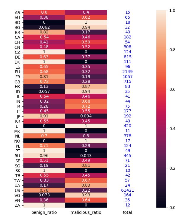
novel features. Finally, the different sets of features were evaluated using well-
known machine learning and deep learning algorithms, which led to a robust and
efficient malicious domain detection system.
     The rest of the paper is organized as follows: Section 2 presents the evaluation
metric used, and Section 3 summarizes related works. Section 4 describes the
methodology and the novel features. Section 5 presents the empirical analysis
and evaluation. Finally, Section 6 concludes and summarizes this work.

2   Evaluation Metrics

Machine Learning (ML) is a subfield of Computer Science aimed at getting
computers to act and improve over time autonomously by feeding them data in
the form of observations and real-world interactions. In contrast to traditional
programming, when one provides input and algorithm and receives an output
when using ML, one provides a list of inputs and their associated outputs, in
order to extract the algorithm that maps the two.
     ML algorithms are often categorized as either supervised or unsupervised. In
supervised learning, each example is a pair consisting of an input vector (also
called data point) and the desired output value (class/label). Unsupervised learn-
ing learns from data that has not been labeled, classified, or categorized. Instead
of responding to feedback, unsupervised learning identifies commonalities in the
data and reacts based on the presence or absence of such commonalities in each
new piece of data.
     In order to evaluate how a supervised model is adapted to a problem, the
dataset needs to be split into two, the training set and the testing set. The
training set is used to train the model, and the testing set is used to evaluate
how well the model "learned" (i.e. by comparing the model predictions with the
known labels). Usually, the train/test distribution is around 75%/25% (depend-
ing on the problem and the amount of data). Standard evaluation criteria are as
follows: Recall, Precision, Accuracy, F1-score, and Loss. All of these criteria can
easily be extracted from the evaluation’s confusion matrix.
     Confusion matrix (Table 1) is commonly used to describe the performance
of a classification model. WLOG, we define positive instances as malicious and
negative as benign. Recall (Eq. 1) is defined as the number of correctly classified
malicious examples out of all the malicious ones. Similarly, Precision (Eq. 2) is
the number of correctly classified malicious examples out of all examples clas-
sified as malicious (both correctly and wrongly classified). Accuracy (Eq. 3) is
used as a statistical measure of how well a classification test correctly identifies
or excludes a condition. That is, the accuracy is the proportion of true results
(both true positives and true negatives) among the total number of cases exam-
ined. Finally, F1-score (Eq. 4) is a measure of a test’s accuracy. It considers both
the precision and the recall of the test to compute the score. The F1-score is the
harmonic average of the precision and recall, where an F1-score reaches its best
value at 1 (perfect precision and recall) and worst at 0. These criteria are used
as the main evaluation metric. Since a classification model is being examined
here, the Logarithmic loss (Eq. 5) was chosen as the loss function.
In this research, the problem of identifying malicious web domains can be
classified as supervised learning, as the correct label (i.e. malicious or benign)
can be extracted using a blacklist-based method, as we describe in the next
chapter.
Prediction Outcome
Positive Negative Total
True False
Actual Positive TP+FN
Positive Negative
Value
False True
Negative FP+TN
Positive Negative
Total P N
Table 1: Confusion Matrix
TP
Recall = (1)
TP + FN
TP TP
P recision = = (2)
TP + FP P
TP + TN T
Accuracy = = (3)
TP + FP + TN + FN P +N
P recision · Recall
F1 − score = 2 · (4)
P recision + Recall
N
1 X
Loss = − (yi · log(pi ) + (1 − yi ) · log(1 − pi )) (5)
N i=1
3 Related Work
The issue of identifying malicious domains is a fundamental problem in cyber-
security. This section discusses recent results in identifying malicious domains,
focusing on three significant methodologies: Mathematical Theory approaches,
ML-based techniques, and Big Data approaches.The use of graph theory to identify malicious domains was more pervasive in
the past [22,28,35,41,64]. Yadav et al. [64] presented a method for recognizing
malicious domain names based on fast flux. Fast flux is a DNS technique used
by botnets to hide phishing and malware delivery sites behind an ever-changing
network of compromised hosts acting as proxies. Their methodology analyzed
the DNS queries and responses to detect if and when domain names are being
generated by a Domain Generation Algorithm (DGA). Their solution was based
on computing the distribution of alphanumeric characters for groups of domains
and by statistical metrics with the KL (Kullback Leibler) distance, Edit distance
and Jaccard measure to identify these domains. Their results for a fast-flux
attack using the Jaccard Index achieved impressive results, with 100% detection
and 0% false positives. However, for smaller numbers of generated domains for
each TLD, their false positive results were much higher, at 15% when 50 domains
were generated for the TLD using the KL-divergence over unigrams, and 8%
when 200 domains were generated for each TLD using Edit distance.
Dolberg et al. [22] described a system called Multi-dimensional Aggregation
Monitoring (MAM) that detects anomalies in DNS data by measuring and com-
paring a âĂIJsteadinessâĂİ metric over time for domain names and IP addresses
using a tree-based mechanism. The steadiness metric is based on a similar do-
main to IP resolution patterns when comparing DNS data over a sequence of
consecutive time frames. The domain name to IP mappings were based on an
aggregation scheme and measured steadiness. In terms of detecting malicious
domains, the results showed that an average steadiness value of 0.45 could be
used as a reasonable threshold value, with a 73% true positive rate and only 0.3%
false positives. The steadiness values might not be considered a good indicator
when fewer malicious activities were present (e.g.able results using transductive classifier it managed to achieve high accuracy
and F1-score with 99% and 97.5% respectively.
Bilge et al. [15] created a system called Exposure, designed to detect malicious
domain names. Their system uses passive DNS data collected over some period
of time to extract features related to known malicious and benign domains. Pas-
sive DNS Replication[61,12,13,15,46,37,49] refers to the reconstruction of DNS
zone data by recording and aggregating live DNS queries and responses. Passive
DNS data could be collected without requiring the cooperation of zone adminis-
trators. The Exposure is designed to detect malware- and spam-related domains.
It can also detect malicious fast-flux and DGA-related domains based on their
unique features. The system computes the following four sets of features from
anonymized DNS records: (a) Time-based features related to the periods and
frequencies that a specific domain name was queried in; (b) DNS-answer-based
features calculated based on the number of distinctive resolved IP addresses and
domain names, the countries that the IP addresses reside in, and the ratio of
the resolved IP addresses that can be matched with valid domain names and
other services; (c) TTL-based features that are calculated based on statistical
analysis of the TTL over a given time series; (d) Domain name-based features
are extracted by computing the ratio of the numerical characters to the domain
name string, and the ratio of the size of the longest meaningful substring in
the domain name. Using a Decision Tree model, Exposure reported a total of
100,261 distinct domains as being malicious, which resolved to 19,742 unique
IP addresses. The combination of features that were used to identify malicious
domains led to the successful identification of several domains that were related
to botnets, flux networks, and DGAs, with low false positive and high detection
rates. It may not be possible to generalize the detection rate results reported
by the authors (98%) since they were highly dependent on comparisons with
biased datasets. Despite the positive results, once an identification scheme is
published, it is always possible for an attacker to evade detection by mimicking
the behaviors of benign domains.
Rahbarinia et al. [49] presented a system called Segugio, an anomaly detec-
tion system based on passive DNS traffic to identify malware-controlled domain
names based on their relationship to known malicious domains. The system de-
tects malware-controlled domains by creating a machine domain bipartite graph
that represents the underlying relations between new domains and known be-
nign/malicious domains. The system operates by calculating the following fea-
tures: (a) Machine Behavior, based on the ratio of âĂIJknown maliciousâĂİ and
âĂIJunknownâĂİ domains that query a given domain d over the total number of
machines that query d. The larger the total number of queries and the fraction
of malicious related queries, the higher the probability that d is a malware con-
trolled domain; (b) Domain Activity, where given a time period, domain activity
is computed by counting the total number of days in which a domain was actively
queried; (c) IP Abuse, where given a set of IP addresses that the domain resolves
to, this feature represents the fraction of those IP addresses that were previously
targeted by known malware controlled domains. Using a Random Forest model,Segugio was shown to produce high true positive and very low false positive rates
(94% and 0.1% respectively). It was also able to detect malicious domains earlier
than commercial blacklisting websites. However, Segugio is a system that can
only detect malware related domains based on their relationship to previously
known domains and therefore cannot detect new (unrelated to previous mali-
cious domains) malicious domains. More information about malicious domain
filtering and malicious URL detection can be found in [21,52].
Adversarial Machine Learning is a subfield of Machine Learning in which the
training and testing set do not share the same distribution, for example, given
perturbations on a malicious instance so that it will be falsely classified. These
manipulated instances are commonly called adversarial examples (AE)[24]. AE
are samples an attacker changes, based on some knowledge of the model classifi-
cation function. These examples are slightly different from correctly classified ex-
amples. Therefore, the model fails to classify them correctly. AE are widely used
in the fields of spam filtering[38], network intrusion detection systems (IDS)[23],
Anti-Virus signature tests[39] and bio-metric recognition[51].
Attackers commonly follow one of two models to generate adversarial exam-
ples: 1) white-box attacker[34,48,59], which has full knowledge of the classifier
and the train/test data; 2) black-box attacker[34,42,54], which has access to the
model’s output for each given input.
Various methods emerged to tackle AE-based attacks and make ML models
robust. The most promising are those based on game-theoretic approaches[17,58,65],
robust optimization[34,48,63], and adversarial retraining[32,40,3]. These approaches
mainly concern feature-space models of attacks where feature space models as-
sume that the attacker changes values of features directly. Note that these attacks
may be an abstraction of reality as random modifications to feature values may
not be realizable or avoid the manipulated instance functionality.
Big Data is an evolving term that describes any voluminous amount of struc-
tured, semi-structured and unstructured data that can be mined for information.
Big data is often characterized by 3Vs: the extreme Volume of data, the wide
Variety of data types and the Velocity at which the data must be processed.
To implement Big Data, high volumes of low-density, unstructured data need to
be processed. This can be data of unknown value, such as Twitter data feeds,
click streams on a web page or a mobile app, or sensor enabled equipment. For
some organizations, this might be tens of terabytes of data. For others, it may
be hundreds of petabytes. Velocity is the fast rate at which data are received
and (perhaps) acted on. Normally, the highest velocity of data streams directly
into memory rather than being written to disk.
Torabi et al. [61] surveyed state of the art systems that utilize passive DNS
traffic for the purpose of detecting malicious behaviors on the Internet. They
highlighted the main strengths and weaknesses of these systems in an in depth
analysis of the detection approach, collected data, and detection outcomes. They
showed that almost all systems have implemented supervised machine learning.
In addition, while all these systems require several hours or even days before
detecting threats, they can achieve enhanced performance by implementing asystem prototype that utilizes big data analytic frameworks to detect threats
in near real-time. This overview contributed in four ways to the literature. (1)
They surveyed implemented systems that used passive DNS analysis to detect
DNS abuse/misuse; (2) they performed an in-depth analysis of the systems and
highlighted their strengths and limitations; (3) they implemented a system pro-
totype for near real-time threat detection using a big data analytic framework
and passive DNS traffic; (4) they presented real-life cases of DNS misuse/abuse
to demonstrate the feasibility of a near real time threat detection system pro-
totype. However, the cases that were presented were too specific. In order to
understand the real abilities of their system, the system must be analyzed with
a much larger test dataset.
4 Methodology
The following criteria are used: Section 4.1 outlines the characteristics and meth-
ods of collection of the dataset. Section 4.2, defines each of the well known
features evaluated. Section 4.3 covers the evaluation of their robustness, and
Section 4.4 presents novel features and evaluates their robustness.
4.1 Data Collection
The main ingredient of ML models is the data on which the models are trained.
As discussed above, data collection should be as heterogeneous as possible to
model reality. The data collected for this work include both malicious and be-
nign URLs: the benign URLs are based on the Alexa top 1 million [1], and the
malicious domains were crawled from multiple sources [4,7,5] due to the fact
they are quite rare.
According to [10], 25% of all URLs in 2017 were malicious, suspicious or
moderately risky. Therefore, to make a realistic dataset, all the evaluations in-
clude all 1,356 malicious active unique URLs, and consequently 5,345 benign
active unique URLs as well. For each instance, the URL and domain informa-
tion properties were crawled from Whois, and DNS records. Whois is a widely
used Internet record listing that identifies who owns a domain, how to get in
contact with them, the creation date, update dates, and expiration date of the
domain. Whois records have proven to be extremely useful and have developed
into an essential resource for maintaining the integrity of the domain name reg-
istration and website ownership. Note that according to a study by ICANN 2 [6],
many malicious attackers abuse the Whois system. Hence, only the information
that could not be manipulated was used.
Finally, based on these resources (Whois and DNS records), the following fea-
tures were generated: the length of the domain, the number of consecutive char-
acters, and the entropy of the domain from the URLs’ datasets. Next, the lifetime
of the domain and the active time of domain were calculated from the Whois
2
Internet Corporation for Assigned Names and Numbersdata. Based on the DNS response dataset (a total of 263,223 DNS records), the
number of IP addresses, distinct geolocations of the IP addresses, average Time
to Live (TTL) value, and the Standard deviation of the TTL were extracted. For
extracting the novel features (Section 4.4) Virus Total (VT) [9] and Urlscan [8]
were used, where Urlscan was used to extract parameters such as the IP address
of the page element of the URL.
4.2 Feature Engineering
Based on previous works surveyed, a set of features which are commonly used
for malicious domain classification [12,13,15,46,49,50,52,56,62] were extracted.
Specifically,the following nine features were used as the baseline:
– Length of domain:
Length of domain = length(Domain(i) ) (6)
The length of domain is calculated by the domain name followed by the TLD
(gTLD or ccTLD). Hence, the minimum length of a domain is four since the
domain name needs to be at least one character (most domain names have
at least three characters) and the TLD (gTLD or ccTLD) is composed of at
least three characters (including the dot character) as well. For example, for
the URL http://www.ariel-cyber.co.il, the length of the domain is 17 (the
number of characters for the domain name - "ariel-cyber.co.il").
– Number of consecutive characters:
Number of consecutive characters =
max{consecutive repeated characters in Domain(i) } (7)
The maximum number of consecutive repeated characters in the domain.
This includes the domain name and the TLD (gTLD or ccTLD). For exam-
ple for the domain "aabbbcccc.com" the maximum number of consecutive
repeated characters value is 4.
– Entropy of the domain:
Entropy of the domain =
ni
X count(cij ) count(cij )
− · log (8)
j=1
length(Domain(i) ) length(Domain(i) )
The calculation of the entropy (i.e. Feature 3) for a given domain Domain(i)
consists of ni distinct characters {ci1 , ci2 , . . . , cini }. For example, for the do-
main "google.com" the entropy is
1 1 2 2 3 3
−(5 · ( 10 · log 10 ) + 2 · ( 10 · log 10 ) + 3(· 10 · log 10 )) = 1.25
The domain has 5 characters that appear once (’l’, ’e’, ’.’, ’c’, ’m’), one char-
acter that appears twice (’g’) and one character that appears three times
(’o’).– Number of IP addresses:
Number of IP addresses = kdistinct IP addressesk (9)
The number of distinct IP addresses in the domain’s DNS record. For ex-
ample for the list ["1.1.1.1", "1.1.1.1","2.2.2.2"] the number of distinct IP
addresses is 2.
– Distinct Geo-locations of the IP addresses:
Distinct Geo-locations of the IP addresses =
kdistinct countriesk (10)
For each IP address in the DNS record, the countries for each IP were listed
and the number of countries was counted. For example for the list of IP
addresses ["1.1.1.1", "1.1.1.1","2.2.2.2"] the list of countries is ["Australia",
"Australia", "France"] and the number of distinct countries is 2.
– Mean TTL value:
Mean TTL value =
µ{TTL in DNS records of Domain(i) } (11)
For all the DNS records of the domain in the DNS dataset, the TTL val-
ues were averaged. For example, if 30 checks of some domain’s DNS records
were conducted, and in 20 of these checks the TTL value was "60" and in
10 checks the TTL value was "1200", the mean is 20·60+10·1200
30 = 440.
– Standard deviation of the TTL:
Standard deviation of TTL =
σ{TTL in DNS records of Domain(i) } (12)
For all the DNS records of the domain in the DNS dataset, the standard
deviation of the TTL values were calculated. For the ”Mean TTL value” ex-
ample above, the standard deviation of the TTL values is 537.401.
– Lifetime of domain:
Lifetime of domain =
DateExpiration − DateCreated (13)
The interval between a domain’s expiration date and creation date in years.
For example for the domain "ariel-cyber.co.il", according to Whois informa-
tion, the dates are: Created on 2015-05-14, Expires in 2020-05-14, Updated
on 2015-05-14. Therefore the lifetime of the domain is the number of years
from 2015-05-14 to 2020-05-14; i.e. 5.– Active time of domain:
Active time of domain =
DateU pdated − DateCreated (14)
Similar to the lifetime of a domain, the active time of a domain is calculated
as the interval between a domain’s update date and creation date in years.
Using the same example as for the ”Lifetime of domain”, the active time
of the domain "ariel-cyber.co.il" is the number of years from 2015-05-14 to
2018-06-04; i.e., 3.
4.3 Robust Feature Selection
Next the robustness of the set of features described above was evaluated to filter
those that could significantly harm the classification process given basic manipu-
lations. In the following analysis, the robustness of these features’ is analysed (i.e.
the complexity of manipulating the feature’s values to result in a false classifica-
tion). Table 2 lists the common features along with the mean value and standard
deviation for malicious and benign URLs based on the dataset. Strikingly, the
table shows that some of the features have similar mean values for both benign
and malicious instances. For example, whereas “Distinct geolocations of the IP
addresses” is quite similar for both types of instances (i.e. not effective in mali-
cious domain classification), it is widely used [56,15,13]. Furthermore, whereas
“Standard deviation of the TTL” has distinct values for benign and malicious
domains, it is shown that an intelligent adversary can easily manipulate this
feature, leading to a benign classification of malicious domains.
Feature Benign mean (std) Malicious mean (std)
Length of domain 14.38 (4.06) 15.54 (4.09)
Number of consecutive characters 1.29 (0.46) 1.46 (0.5)
Entropy of the domain 4.85 (1.18) 5.16 (1.34)
Number of IP addresses 2.09 (1.25) 1.94 (0.94)
Distinct geolocations of the IP addresses 1.00 (0.17) 1.02 (0.31)
Mean TTL value 7,578.13 (17,781.47) 8,039.92 (15,466.29)
Standard deviation of the TTL 2,971.65 (8,777.26) 2,531.38 (7,456.62)
Lifetime of domain 10.98 (7.46) 6.75 (5.77)
Active time of domain 8.40 (6.79) 4.64 (5.66)
Table 2: Classic features - statistical properties
In order to understand the malicious abilities of an adversary, the base fea-
tures were manipulated over a wide range of possible values, one feature at atime.3 For each feature only the range of possible values were taken into ac-
count. This analysis considers an intelligent adversary with black-box access to
the model (i.e. a set of features or output for a given input). The robustness anal-
ysis is based on an ANN model that classifies the manipulated samples, where
the train set is the empirically crawled data, and the test set includes the manip-
ulated malicious samples. Figure 2 depicts the possible adversary manipulations
over any of the features. The evaluation metric, the prediction percentage, was
defined as the average detection rate after modification.
Fig. 2: Base feature manipulation graphs (* robust or semi-robust features)
The well-known features were divided into three groups: robust features,
robust features that seemed non-robust (defined as semi-robust), and non-robust
features. Next, it can be seen how an attacker can manipulate the classifier for
each feature and define its robustness:
1. ”Length of domain”: an adversary can easily purchase a short or long
domain to result in a benign classification for a malicious domain; hence this
feature was classified as non-robust.
2. ”Number of consecutive characters”: surprisingly, as depicted in Fig-
ure 2, manipulating the ”Number of consecutive characters” feature can sig-
3
Each feature was evaluated over all possible values for that feature.nificantly lower the prediction percentage (e.g., move from three consecutive
characters to one or two). Nevertheless, as depicted in Table 2, on average,
there were 1.46 consecutive characters in malicious domains. Therefore, ma-
nipulating this feature is not enough to break the model, and it is considered
to be a robust feature.
3. ”Entropy of the domain”: in order to manipulate the ”Entropy of the do-
main” feature as benign domain entropy, the adversary can create a domain
name with entropy < 4. Take, for example, the domain âĂIJddcd.ccâĂİ
which is available for purchase. The entropy for this domain is 3.54. This
value falls precisely in the entropy area of the benign domains defined by
the trained model. This example breaks the model and causes a malicious
domain to look like a benign URL. Hence, this feature was classified as non-
robust.
4. ”Number of IP addresses”: note that an adversary can add many A
records to the DNS zone file of its domain to imitate a benign domain.
Thus, to manipulate the number of IP addresses, an intelligent adversary
only needs to have several different IP addresses and add them to the zone
file. This fact classifies this feature as non-robust.
5. ”Distinct Geolocations of the IP addresses”: in order to be able to
break the model with the ”Distinct Geolocations of the IP addresses” feature,
the adversary needs to use several IP addresses from different geolocations.
If the adversary can determine how many different countries are sufficient
to mimic the number of distinct countries of benign domains, he will be
able to append this number of IP addresses (a different IP address from
each geo-location) to the DNS zone file. Thus, this feature was also classified
as non-robust. ”Mean TTL value” and ”Standard deviation of the
TTL”: there is a clear correlation between the ”Mean TTL value” and the
”Standard deviation of the TTL” features since the value manipulated by
the adversary is the TTL itself. Thus, it makes no difference if the adversary
cannot manipulate the ”Mean TTL value” feature if the model uses both.
In order to robustify the more, it is better to use the ”Mean TTL value”
feature without the ”Standard deviation of the TTL” one. Solely in terms of
the ”Mean TTL value” feature, Figure 2 shows that manipulation will not
result in a false classification since the prediction percentage does not drop
dramatically, even when this feature is drastically manipulated. Therefore
this feature is considered to be robust.
An adversary can set the DNS TTL values to [0,120000] (according to the
RFC 2181 [2] the TTL value range is from 0 to 231 − 1). Figure 2 shows
that even manipulating the value of this feature to 60000 will break the
model and cause a malicious domain to be wrongly classified as a benign
URL. Therefore the ”Standard deviation of the TTL” cannot be considered
a robust feature.
6. ”Lifetime of domain”: As for the lifetime of domains, based on [56] we
know that a benign domain’s lifetime is typically much longer than a ma-
licious domain’s lifetime. In order to break the model by manipulating the
”Lifetime of domain” feature, the adversary must buy an old domain that isavailable on the market. Even though it is possible to buy an appropriate
domain, it will take time to find one, and it will be expensive. Hence we
considered this to be a semi-robust feature.
7. ”Active time of domain”: Similar to the previous feature, in order to break
”Active time of domain”, an adversary must find a domain with a particular
active time (Figure 2), which is much more tricky. It is hard, expensive,
and possibly unfeasible. Therefore this was considered to be a semi-robust
feature.
Based on the analysis above, the robust features from Table 2 were selected,
and the non-robust ones were dropped. Using that subset the model was trained
and an accuracy of 95.71% with an F1-score of 88.78% was achieved can be
improved. Therefore, we extended our analysis and searched for new features
that would meet the robustness requirements to build a robust model with a
higher F1-score, ending up with a model that results in an accuracy of 99.36%
and F1-score of 98.42%.
4.4 Novel Features
This section presents four novel features which are both robust, and improve the
model’s efficiency.
As stated above, mimicking benign URLs in order to bypass is a mammoth
problem. The aim of the research was to validate that manipulating the features
in order to result in misclassification of malicious instances will require a dis-
proportionate effort that will deter the attacker from doing so. The four novel
features were designed according to this paradigm based on two communication
information properties, passive DNS changes, and the remaining time of SSL cer-
tificate. For each IP, Urlscan extract the geo-location, which in turn is appended
to a communication country list. Similarly, the communication ASNs is a list
of ASNs, that was extracted using Urlscan, each IP address, and appended the
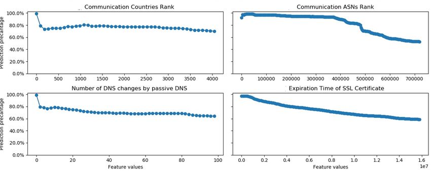
ASNs list. Using the URL dataset and the Urlscan service, benign-malicious ratio
tables for communication countries and for communication ASNs (Figures 3,4)
were created. The ratio tables were calculated for each element E (country - for
the communication countries ratio table, or ASN - for the communication ASNs
ratio table). Each table represents the probability that a URL associated with a
country (ASN) is malicious. In order to extract those probabilities, the number
of malicious URLs associated with E was divided by the total URLs associated
with E. Initially, due to the heterogeneity of the dataset (i.e. there exist some
elements that appear only a few times), the ratio tables were seen to be biased.
To overcome this challenge, an initial threshold was set as an insertion criteria
which is later detailed in Algorithm 1 (CRA).
The following is a detailed summary of the novel features:
– Communication Countries Rank (CCR):
CCR =
CRA(the communication countries list of U RL(i) ) (15)Fig. 3: Communication Countries Ratio
Fig. 4: Communication ASNs Ratio
This feature looks at the communication countries with respect to the com-
  munication IPs, and uses the countries ratio table to rank a specific URL.
– Communication ASNs Rank (CAR):

      CAR =
                         CRA(the communication ASNs list of U RL(i) ) (16)

  Similarly, this feature analyzes the communication ASNs with respect to the
  communication IPs, and uses the ASNs ratio table to rank a specific URL.
  While there is some correlation between the ASNs and the countries, the
  second feature examines each AS (usually ISPs or large companies) within
  each country to gain a wider perspective.
– Number of passive DNS changes:

      P DN S =
                        count(list of passive DNS records of Domain(i) ) (17)

  When inspecting the passive DNS records, benign domains emerged as hav-
  ing much larger DNS changes that the sensors (of the company that collects
  the DNS records) could identify, unlike malicious domains (i.e. 26.4 vs. 8.01,
  as reported in Table 3).
  For the âĂİNumber of passive DNS changesâĂİ the number of DNS records
  changes were counted, which is somewhat similar to other features described
  in [61,12]. Still, these features require much more elaborated information
  which is not publicly available. On the other hand, this feature can be ex-
  tracted from passive DNS records obtained from VirusTotal, which are scarce
  (in terms of record types).
– Remaining time of SSL certificate:

      SSL = Certif icateV alid ·
                          · (Certif icateExpiration − Certif icateU pdated ) (18)

  When installing an SSL certificate, there is a validation process conducted
  by a Certificate Authority (CA). Depending on the type of certificate, the
  CA verifies the organization’s identity before issuing the certificate. When
  analyzing our data it was noted that most of the malicious domains do not
  use valid SSL certificates and those that do only use one for a short period.
  Therefore, this feature was engineered which represents the time the SSL
  certificate remains valid.
  For the âĂİRemaining time of SSL certificateâĂİ, in contrast to a binary
  feature version used by [50], this feature extends the scope and represents
  both the existence of an SSL certificate and the remaining time until the
  SSL certificate expires.
Algorithm 1 Communication Rank
Input: URL, Threshold, Type
Output: Rank (CCR or CAR)
1: if Type = Countries then
2: ItemsList = communication countries list of the URL
3: else
4: ItemsList = ASNs list of the URL
5: end if
6: Rank = 0
7: for Item in ItemsList do
8: Ratio = 0.75 {Init value}
9: T otal_norm = 1 {Init value}
10: if T otalOccurrences(Item) >= T hreshold then
11: T otal_norm = N ormalize(Item)
12: Ratio = BenignRatio(Item)
13: end if
14: Rank+ = (log0.5 (Ratio + )/T otal_norm)
15: end for
The CRA (Algorithm 1) gets a URL as an input and returns its country
communication rate or the ASN communication rate (based on the type in the
input of the algorithm).
For each item (i.e., country or ASN), first the algorithm initialized the value
of the ratio variable to 0.75 (according to [10], 25% of all URLs in 2017 were
malicious, suspicious or moderately risky) and the normalized total occurrences
(Total_norm) of an item to be 1. Next, in Step 9, if the total number of oc-
currences of an item was ≥ to the threshold, the algorithm replaced the ratio
and normalized occurrences to the correct values according to the ratio tables
given in Figures 3 and 4. Finally, the algorithm sums the rank with a log base
0.5 of the ratio (+ some epsilon) and divide this value by the normalized total
occurrences.
Feature Benign mean (std) Malicious mean
(std)
Communication Countries Rank (CCR) 31.31 (91.16) 59.40 (215.15)
Communication ASNs Rank (CAR) 935.59 (12,258.99) 12,979.38 (46,384.86)
Number of passive DNS changes 26.40 (111.99) 8.01 (16.63)
Remaining time of SSL certificate 1.547E7 (2.304E7) 4.365E6 (1.545E7)
Table 3: Novel features - statistical properties
Figure 5 depicts the prediction percentage as a function of changing the novel
features values for each feature in Table 3, Similar to the analysis in Section 4.3.
This evaluation proves that manipulating the values of the novel features doesFig. 5: Novel robust feature manipulation graphs
not break the robust model (i.e., the prediction percentage remains steady).
While one may be concerned by the negative correlation between ”Remaining
time of SSL certificate” feature and the prediction percentage, note that the
average value for malicious domains is three times higher than the benign ones.
While theoretically the adversary can lower this value, the implications of such
action are acquiring (or use some free solution) an SSL certificate. Since there is
a validation process, this process will cause the adversary to lose its anonymity
and be identified.
5 Empirical Analysis and Evaluation
This section describes the testbed used for the evaluation of models based on the
types of features (both robust and not). General settings are provided for each
of the models (e.g. the division of the data into training and test set), as are
the parameters used to configure each of the models, followed by the efficiency
of each model. 4
5.1 Experimental Design
Apart from intelligently choosing the model parameters, one should verify that
the data used for the learning phase accurately represents the real-world distri-
bution of domain malware. Hence, the dataset was constructed such that 75%
were benign domains, and the remaining 25% were malicious domains (~5,000
benign URLs and ~1,350 malicious domains respectively) [10].
There are many ways to define the efficiency of a model. To account for
most of them, a broad set of metrics was extracted including accuracy, recall,
4
Our code is publicly available at https://github.com/nitayhas/
robust-malicious-url-detectionF1-score, and training time. Note that for each model, the dataset was split
into train and test sets where 75% of the data (both benign and malicious) was
randomly assigned to the train test, and the remaining domains are assigned to
the test set.
The evaluation step measured the efficiency of the different models while
varying the robustness of the features included in the model. Specifically, four
different models (i.e. Logistic Regression, SVM, ELM, and ANN) were trained
using the following feature sets:
– Base (B ) - The set of commonly used features in previous works (see Table 2
for more details).
– Base Robust (BR) - the subset of robust base features (marked with a * in
Figure 2).
– ”TCP” (TCP ) - The four novel features: Time of SSL certificate, Communi-
cation ranks (CCR and CAR) and PassiveDNS changes (see Table 3).
– Base Robust + ”TCP”(BRTCP ) - the union of BR and TCP, the robust
subset of all features.
– Base + ”TCP” (BTCP ) - the union of B and TCP.
Recall that feature sets (i.e. TCP, BRTCP, and BTCP) which are based on
the novel features (i.e. CCR and CAR) , require communication ratio tables.
Hence, to keep the models unbiased (i.e. omit the data that was used for gener-
ating the ratio tables from the learning process), it was necessary allocate some
of the data to creation of the ratio tables. Due to the variety of countries and
ASNs, it was decided to dedicate the majority of the data to this process. For the
evaluation, the dataset was split into two parts: when using the novel features
75% of the data was used to create the ratio tables and the remaining 25% of
the data was used to extract the features, train and test for the models, as can
be seen in Figure 6a. In the case of using the well-known features, 100% of the
data was used for the feature extraction as can be seen in Figure 6b. Evaluations
for the opposite split ratio (i.e. 25/75) were also conducted, this time allocat-
ing most of the data to the learning phase. The findings showed that the trend
between these two ratios was similar (as presented in Section 5.2). Both ratios
returned high results but, for most of the models, the 75/25 ratio returned a
higher F1-Score and higher Recall measures (e.g. LR, SVM, and ANN for each
feature set). For the 25/75 distribution, the F1-Score and the Recall measures
were only higher for the ELM (around 1%-2% higher). Therefore, while both
results are reported in the end of this section, WLOG, the main focus of the
discussion is on the 75/25 distribution.
5.2 Models and Parameters
Four commonly used classification models are analyzed: Logistic Regression
(LR), Support Vector Machines (SVM), Extreme Learning Machine (ELM), and
Artificial Neural Networks (ANN). All the models were trained and evaluated
on a Dell XPS 8920 computer, Windows 10 64Bit OS with 3.60GHz Intel Core
i7-7700 CPU, 16GB of RAM, and NVIDIA GeForce GTX 1060 6GB.(a) Data distribution while using our novel (b) Data distribution while using only the
features base features
Fig. 6: Data Distribution
In the following paragraphs, for each model, the hyperparameters used for
the evaluation are first described, followed by the empirical, experimental results
(which sums up several test results using different random train-test sets), and
a short discussion of the findings and their implications.
Logistic Regression As a baseline for the evaluation process, and before us-
ing the nonlinear models, the LR classification model was used. The LR model
with the five feature sets was trained and the hyperparameters were tuned to
maximize the model’s performance.
Hyperparameters: Polynomial degree: 3;K-Fold Cross-Validation k=10;
Solver: L-BFGS [33].
Table 4 shows that the different feature sets resulted in similar accuracy
rates. However, the accuracy rate measures how well the model predicts (i.e.
TP+TN) with respect to all the predictions (i.e. TP+TN+FP+FN). Thus given
the unbalanced dataset (75% of the dataset are benign and 25% are malicious
domains), ~90% accuracy is not necessarily a sufficient result in terms of malware
detection. For example, the TCP feature set has high accuracy but in contrast a
very poor F1-Score, due to the high Precision rate and poor Recall rate (which
represents the ratio of malicious instances detected). As the recall is low for all
features sets, this work demonstrates that accuracy rate is not a good measure in
this domain; therefore, it was decided to focus on the F1-score measure, which is
the harmonic mean of the precision and the recall measures. Next, it was decided
to use the SVM model with an RBF kernel as a nonlinear model.
Support Vector Machine (SVM) Hyperparameters: Polynomial degree:
3; K-Fold Cross-Validation k=10; γ=2; Kernel: RBF [44].
Compared to the results of the LR model (Table 4), the results of the SVM
model (Table 5) show a significant improvement in the recall and F1-score mea-
sures; e.g. for Base, the recall and the F1-score measures were both above 90%.
One could be concerned by the fact that the model trained on the Base feature
set resulted in a higher recall (and F1-score) compare to the one trained on
the Robust Base feature set. However, it should be noted that the Robust Basefeature set is robust to adversarial manipulation and uses less than half of the
features provided in the training phase with the Base feature set. This discus-
sion also applies to the BRTCP and BTCP feature sets. Another advantage of
including the novel features is the fact that models converge much faster.
The results are based on analyzing a non-manipulated dataset. As stated
above, the Base feature set includes some non-robust features. Hence, an in-
telligent adversary can manipulate the values of these features, resulting in a
wrong classification of malicious instances (up to the extreme of a 0% recall).
However, an intelligent adversary should invest much more effort for a model
that was trained using the Robust Base or TCP features, since each of them
was specifically chosen to avoid such manipulations. In order to find models that
were also efficient on the non-manipulated dataset, the two sophisticated models
were examined in the analysis, the ELM model as presented in [56] and the ANN
model.
Feature set Accuracy Recall F1-Score
Base 89.99% 38.82% 53.21%
Robust Base 88.33% 38.87% 49.42%
TCP 86.20% 8.30% 14.99%
BRTCP 88.82% 52.46% 65.57%
BTCP 92.86% 64.14% 72.48%
Table 4: Model performance - Logistic Regression (in %)
Feature set Accuracy Recall F1-Score
Base 96.49% 91.20% 91.36%
Robust Base 90.14% 56.51% 69.93%
TCP 83.10% 60.21% 54.21%
BRTCP 96.78% 91.37% 92.02%
BTCP 97.95% 90.73% 92.83%
Table 5: Model performance - SVM (in %)
ELM Hyperparameters: One input layer, one hidden layer, and one output
layer. Activation function: first layer - ReLU [36]; hidden layer - Sigmoid. K-Fold
Cross-Validation k=10 [56]. Overall, the ELM model resulted in high accuracy
and higher Recall rates compared to Table 4, for any feature set. When compared
to the SVM models, the Base model resulted in lower recall (though a higher
F1-score was achieved with the ELM model). On the other hand, the RobustBase resulted in a higher recall in the ELM model compared to the SVM one.
Even though the Robust Base feature set had a low dimensional space, the three
rates (i.e. Accuracy, Recall, and F1-score) were higher than those of the Base
feature set. Moving to the sets that include the novel features increased these
metrics, while improving the robustness of the model at the same time.
Feature set Accuracy Recall F1-Score
Base 98.17% 88.81% 92.92%
Robust Base 98.83% 92.24% 95.81%
TCP 98.88% 94.64% 96.84%
BRTCP 98.86% 95.82% 97.07%
BTCP 98.19% 93.09% 95.34%
Table 6: Model performance - ELM (in %)
ANN Hyperparameters: One input layer, three hidden layers, and one out-
put layer. Activation function: first layer - ReLU; first hidden layer - RELU;
Second hidden layer - LeakyReLU; Third hidden layer - Sigmoid. Batch size
-150, learning rate of 0.01; Solver: Adam [30] with β1 = 0.9 and β2 = 0.999.
K-Fold Cross-Validation k=10. Similarl to the ELM results, the ANN results
show high performance on all feature sets. For the “basic” feature sets (i.e. Base
and Robust Base) the ELM models resulted in higher recall and F1-score. Still,
the main focus was in the BTCP feature set and more specifically in the BRTCP
variant, and for those feature sets, the ANN models resulted in higher recall and
F1-score.
Feature set Accuracy Recall F1-Score
Base 97.20% 88.03% 90.23%
Robust Base 95.71% 83.63% 88.78%
TCP 98.03% 96.83% 95.24%
BRTCP 99.36% 98.77% 98.42%
BTCP 99.82% 99.47% 99.56%
Table 7: Model performance - ANN (in %)
Discussion This analysis conclude with Figure 7 and Tables 8, 9 and 10 that
summarize the evaluation. In particular, Figure 7 shows the overall results and
presents the F1-scores of the feature sets for all the models.Fig. 7: The F1-Score by feature sets and models
aa
aa Feature set
aa Base Base Robust
aa
Model aa
Accuracy: 0.90 Accuracy: 0.88
Precision: 0.84 Precision: 0.68
Recall: 0.39 Recall: 0.39
Logistic
F1-score: 0.53 F1-score: 0.49
Regression
Loss: 3.45 Loss: 4.03
AUC: 0.85 AUC: 0.81
Accuracy: 0.96 Accuracy: 0.90
Precision: 0.91 Precision: 0.91
Recall: 0.91 Recall: 0.56
SVM
F1-score: 0.91 F1-score: 0.69
Loss: 1.20 Loss: 3.40
AUC: 0.96 AUC: 0.92
Accuracy: 0.98 Accuracy: 0.98
Precision: 0.98 Precision: 0.99
Recall: 0.88 Recall: 0.92
ELM
F1-score: 0.92 F1-score: 0.95
Loss: 0.63 Loss: 0.40
AUC: 0.99 AUC: 0.99
Accuracy: 0.97 Accuracy: 0.95
Precision: 0.92 Precision: 0.94
Recall: 0.88 Recall: 0.83
ANN
F1-score: 0.90 F1-score: 0.88
Loss: 0.44 Loss: 0.68
AUC: 0.98 AUC: 0.97
Table 8: Raw data results for the models that trained with the base features
(100% of the dataset records)Tables 8-10 depicts all the evaluation matrices (i.e. accuracy, precision, recall,
F1-score, loss, and AUC). While Table 9 depicts the models’ performance where
75% of the data was used to construct the ratio table, Table 10 depicts the
performance where the minority of data (i.e. 25%) was used to construct the
ratio tables. Looking at the resultant recall and F1-score, it seems that models
analyzed in Table 9, in which most of the data is dedicated to the ratio tables
(i.e. to the TCP features), resulted in higher performance, even though these
models had one third of the data available to the models evaluated in Table 10.
At the same time, it is important to note that the best model resulted by using
the Base Robust + TCP features, to train the ELM model and dedicating 25% of
the data to the feature engineering phase, and the reminder 75% to the learning
process.
All the results provided above are based on clean data (i.e. with no adversar-
ial manipulation). Naturally, given an adversarial model where the attacker can
manipulate the values of features, models which are based on the Robust Base or
TCP feature sets will dominate models that are trained using the Base dataset.
Thus, by showing that the Robust Base feature set does not dramatically de-
crease the performance of the classifier using clean data, and that adding the
novel feature improves the model’s performance as well as its robustness, the
conclusion is that malicious domain classifiers should use this feature set for
robust malicious domain detection.
6 Conclusion
Numerous attempts have been made to tackle the problem of identifying ma-
licious domains. However, many of them fail to successfully classify malware
in realistic environments where an adversary can manipulate the URLs and/or
other extracted features. Specifically, this research tackled the case where an at-
tacker has access to the model (i.e. a set of features or output for a given input),
and tampers with the domain properties. This tampering has a catastrophic
effect on the modelâĂŹs efficiency. As a countermeasure, an intelligent feature
selection procedure was used which is robust to adversarial manipulation as well
as inclusion of novel robust features. Feature robustness and model effectiveness
were evaluated based on well known machine and deep learning models over a
sizeable realistic dataset.
The evaluation showed that models that are trained using the robust features
are more precise in terms of manipulated data while maintaining good results on
clean data as well. Clearly, further research is needed to create models that can
also classify malicious domains into malicious attack types. Another promising
direction would be clustering a set of malicious domains into one cyber campaign.
References
1. Alexa, https://www.alexa.com
2. Clarifications to the dns specification, https://tools.ietf.org/html/rfc2181Model/Feature set TCP Base Robust + TCP Base + TCP
Accuracy: 0.86 Accuracy: 0.88 Accuracy: 0.92
Precision: 0.77 Precision: 0.87 Precision: 0.83
Recall: 0.08 Recall: 0.52 Recall: 0.64
Logistic Regression
F1-score: 0.15 F1-score: 0.65 F1-score: 0.72
Loss: 4.76 Loss: 3.86 Loss: 2.46
AUC: 0.79 AUC: 0.93 AUC: 0.94
Accuracy: 0.83 Accuracy: 0.96 Accuracy: 0.97
Precision: 0.60 Precision: 0.92 Precision: 0.95
Recall: 0.49 Recall: 0.91 Recall: 0.90
SVM
F1-score: 0.54 F1-score: 0.92 F1-score: 0.92
Loss: 5.83 Loss: 1.11 Loss: 0.70
AUC: 0.80 AUC: 0.98 AUC: 0.98
Accuracy: 0.98 Accuracy: 0.98 Accuracy: 0.98
Precision: 0.99 Precision: 0.98 Precision: 0.97
Recall: 0.94 Recall: 0.95 Recall: 0.93
ELM
F1-score: 0.96 F1-score: 0.97 F1-score: 0.95
Loss: 0.38 Loss: 0.39 Loss: 0.62
AUC: 0.99 AUC: 0.99 AUC: 0.98
Accuracy: 0.98 Accuracy: 0.99 Accuracy: 0.99
Precision: 0.93 Precision: 0.98 Precision: 0.99
Recall: 0.96 Recall: 0.98 Recall: 0.99
ANN
F1-score: 0.95 F1-score: 0.98 F1-score: 0.99
Loss: 0.31 Loss: 0.10 Loss: 0.02
AUC: 0.99 AUC: 0.99 AUC: 0.99
Table 9: Raw data results for the models that trained on the 75/25 dataset
distribution, 42,578/10,979 URLs (ratio tables/feature extraction)Model/Feature set TCP Base Robust + TCP Base + TCP
Accuracy: 0.82 Accuracy: 0.87 Accuracy: 0.90
Precision: 0.80 Precision: 0.85 Precision: 0.82
Recall: 0.07 Recall: 0.39 Recall: 0.57
Logistic Regression
F1-score: 0.13 F1-score: 0.53 F1-score: 0.68
Loss: 5.94 Loss: 4.24 Loss: 3.42
AUC: 0.70 AUC: 0.89 AUC: 0.93
Accuracy: 0.82 Accuracy: 0.91 Accuracy: 0.96
Precision: 0.89 Precision: 0.81 Precision: 0.91
Recall: 0.07 Recall: 0.65 Recall: 0.87
SVM
F1-score: 0.13 F1-score: 0.72 F1-score: 0.89
Loss: 5.88 Loss: 3.09 Loss: 1.33
AUC: 0.76 AUC: 0.94 AUC: 0.97
Accuracy: 0.99 Accuracy: 0.99 Accuracy: 0.98
Precision: 0.99 Precision: 0.99 Precision: 0.97
Recall: 0.96 Recall: 0.98 Recall: 0.93
ELM
F1-score: 0.97 F1-score: 0.98 F1-score: 0.95
Loss: 0.25 Loss: 0.16 Loss: 0.54
AUC: 0.99 AUC: 0.99 AUC: 0.99
Accuracy: 0.94 Accuracy: 0.98 Accuracy: 0.98
Precision: 0.99 Precision: 0.99 Precision: 0.97
Recall: 0.72 Recall: 0.90 Recall: 0.95
ANN
F1-score: 0.83 F1-score: 0.94 F1-score: 0.96
Loss: 0.81 Loss: 0.31 Loss: 0.18
AUC: 0.97 AUC: 0.99 AUC: 0.99
Table 10: Raw data results for the models that trained on the 25/75 dataset
distribution 10,979/42,578 URLs (ratio tables/feature extraction)3. improving robustness of ml classifiers against realizable evasion attacks using con-
served features
4. Phishtank, https://www.phishtank.com
5. Scumware, https://www.scumware.org
6. A study of whois privacy and proxy service abuse, https://gnso.icann.org/
sites/default/files/filefield_41831/pp-abuse-study-20sep13-en.pdf
7. Url abuse, https://urlhaus.abuse.ch
8. urlscan.io, https://www.urlscan.io
9. Virustotal, https://www.virustotal.com
10. Webroot, https://www-cdn.webroot.com/9315/2354/6488/
2018-Webroot-Threat-Report_US-ONLINE.pdf
11. Ahmed, M., Khan, A., Saleem, O., Haris, M.: A fault tolerant approach for ma-
licious url filtering. In: International Symposium on Networks, Computers and
Communications. pp. 1–6 (2018)
12. Antonakakis, M., Perdisci, R., Dagon, D., Lee, W., Feamster, N.: Building a dy-
namic reputation system for dns. In: USENIX. pp. 273–290 (2010)
13. Antonakakis, M., Perdisci, R., Lee, W., Vasiloglou, N., Dagon, D.: Detecting mal-
ware domains at the upper dns hierarchy. In: USENIX. vol. 11, pp. 1–16 (2011)
14. Berger, H., Dvir, A.Z., Geva, M.: A wrinkle in time: A case study in DNS poisoning.
CoRR (2019), http://arxiv.org/abs/1906.10928
15. Bilge, L., Sen, S., Balzarotti, D., Kirda, E., Kruegel, C.: Exposure: A passive dns
analysis service to detect and report malicious domains. Trans. Inf. Syst. Secur.
16(4), 1–28 (2014)
16. Blum, A., Wardman, B., Solorio, T., Warner, G.: Lexical feature based phishing
url detection using online learning. In: Workshop on Artificial Intelligence and
Security. pp. 54–60 (2010)
17. Brückner, M., Scheffer, T.: Stackelberg games for adversarial prediction problems.
In: International Conference on Knowledge Discovery and Data Mining. pp. 547–
555 (2011)
18. Caglayan, A., Toothaker, M., Drapeau, D., Burke, D., Eaton, G.: Real-time detec-
tion of fast flux service networks. In: Conference For Homeland Security, Cyberse-
curity Applications & Technology. pp. 285–292 (2009)
19. Canali, D., Cova, M., Vigna, G., Kruegel, C.: Prophiler: a fast filter for the large-
scale detection of malicious web pages. In: International Conference on World Wide
Web. pp. 197–206 (2011)
20. Choi, H., Zhu, B.B., Lee, H.: Detecting malicious web links and identifying their
attack types. WebApps 11(11), 218 (2011)
21. Das, A., Data, G., Platform, A., Jain, E., Dey, S.: Machine learning features for
malicious url filtering–the survey (2019)
22. Dolberg, L., François, J., Engel, T.: Efficient multidimensional aggregation for large
scale monitoring. In: LISA. pp. 163–180 (2012)
23. Fogla, P., Sharif, M.I., Perdisci, R., Kolesnikov, O.M., Lee, W.: Polymorphic blend-
ing attacks. In: USENIX. pp. 241–256 (2006)
24. Goodfellow, I.J., Shlens, J., Szegedy, C.: Explaining and harnessing adversarial
examples. arXiv preprint:1412.6572 (2014)
25. Harel, N., Dvir, A., Dubin, R., Barkan, R., Shalala, R., Hadar, O.: Misal-a minimal
quality representation switch logic for adaptive streaming. Multimedia Tools and
Applications (2019)
26. Hu, Z., Chiong, R., Pranata, I., Susilo, W., Bao, Y.: Identifying malicious web
domains using machine learning techniques with online credibility and performance
data. In: Congress on Evolutionary Computation (CEC). pp. 5186–5194 (2016)You can also read