Deep Neural Networks for Active Wave Breaking Classification
←
→
Page content transcription
If your browser does not render page correctly, please read the page content below
Deep Neural Networks for Active Wave Breaking
                                                 Classification
                                                 Caio E. Stringari1,* , Pedro V. Guimarães1,2,+ , Jean-François Filipot1,+ , Fabien Leckler1, ,
                                                 and Rui Duarte1,

                                                 1 France Energies Marines, Plouzané, 29280, France
                                                 2 PPGOceano,    Federal University of Santa Catarina, Florianópolis, 88040-900, Brazil
                                                 * Caio.Stringari@france-energies-marines.com
arXiv:2101.11478v1 [physics.ao-ph] 27 Jan 2021

                                                 + these authors contributed equally to this work

                                                 ABSTRACT

                                                 Wave breaking is an important process for energy dissipation in the open ocean and coastal seas.
                                                 It drives beach morphodynamics, controls air-sea interactions, determines when ship and offshore
                                                 structure operations can occur safely, and influences on the retrieval of ocean properties from satellites.
                                                 Still, wave breaking lacks a proper physical understanding mainly due to scarce observational field data.
                                                 Consequently, new methods and data are required to improve our current understanding of this process.
                                                 In this paper we present a novel machine learning method to detect active wave breaking, that is, waves
                                                 that are actively generating visible bubble entrainment in video imagery data. The present method
                                                 is based on classical machine learning and deep learning techniques and is made freely available to
                                                 the community alongside this publication. The results indicate that our best performing model had
                                                 a balanced classification accuracy score of ≈ 90% when classifying active wave breaking in the test
                                                 dataset. An example of a direct application of the method includes a statistical description of geometrical
                                                 and kinematic properties of breaking waves. We expect that the present method and the associated
                                                 dataset will be crucial for future research related to wave breaking in several areas of research, which
                                                 include but are not limited to: improving operational forecast models, developing risk assessment and
                                                 coastal management tools, and refining the retrieval of remotely sensed ocean properties.

                                                 Introduction

                                                 Wave breaking is one of the most challenging water wave phenomena to investigate. Despite nearly
                                                 two centuries of research, the current practical description of the process is still mostly empirical1–4 .
                                                 Precise wave breaking modelling requires explicit knowledge of the wave phase speed and the fluid
                                                 velocity distribution on the wave crest which can only be done by numerically solving the Navier-Stokes
                                                 equations in a framework that currently is too computationally expensive for practical applications5 .
                                                 Consequently, current large-scale state-of-the-art wave models rely on statistical approaches (mostly
the spectral approach) to represent the waves6–8 . This type of models parameterizes wave breaking as
a function of known parameters such as the wind speed6 , the local wave height to water depth ratio7
or semi-empirical breaking wave height probability distributions2, 9 . Due to a lack of observed data,
the constants involved in these models have been derived from limited datasets that may not adequately
represent the natural environment. For example, a recent study has shown that popular surf zone parametric
wave breaking models incorrectly represented the fraction of broken waves in their formulations with
errors >50%, despite these models being able to adequately represent surf zone energy dissipation possibly
due to parameter tuning10 . This paper aims to start addressing the data unavailability issue by providing a
reliable and reproducible method to detect and track waves that are actively breaking in video imagery
data.

   Wave breaking directly affects several environmental phenomena. For example, wave breaking is
considered as the main driver for air-sea exchanges11 , being often described as a function of Phillips’12
Λ(c)dc parameter. This parameter is defined as the average total length per unit surface area of breaking
fronts that have velocities in the range c to c + dc and its moments are assumed to correspond to different
phenomena such as whitecap coverage (second moment), rate of air entrainment (third moment), and
momentum flux (fourth moment). As previously identified13 , different interpretations of how data is
processed to obtain Λ(c)dc resulted in differences of 175% in the first moment and 300% in the fifth
moment of Λ(c)13, 14 . This issue does not seem to limit the applicability of Phillips’ framework. A recent
study, for example, used a wave breaking parameterization fully based on Λ(c)dc to derived whitecap
coverage off the coast of California15 . To the authors’ knowledge, however, no study has assessed the
impact that errors in wave breaking detection has on measured Λ(c) distributions and how such errors
would impact on the conclusions that have been drawn from these models (for example, the assumption
that Λ(c) is a simple function of wind speed11 ). More importantly, in the case which new observations
diverge from Phillips’ original theory (as we will later show in this paper), new and improved wave
breaking models will certainly follow.

   Further, breaking waves have a direct impact on the remote sensing of the ocean surface from satellites,
aircraft, or platform mounted instruments. Wave breaking has been observed to significantly modulate
measurements of backscatter off radars with large increases in backscatter being directly correlated with

                                                                                                       2/25
breaking waves16 . Given that part of the data that will be used here (see Methods for details) coincides
with the location of previous wave backscatter studies16 , data derived from our method could to lead
to explicit formulations correlating wave breaking and radar backscatter. Such formulations could, in
the future, lead to more reliable satellite-derived scatterometer data, which currently ignores17 or relies
on empirical wave breaking models18 . The foam generated by breaking waves at the sea surface also
influences on the measurement of microwave brightness temperature signatures for moderate to high wind
speeds19, 20 . To date, no study has, however, systematically quantified such temperature signatures for large
field datasets and most of our knowledge is empirical. Such limitation could be addressed by extending
wave breaking detection and tracking methods to infrared wavelengths, which is directly correlated to
water temperature21 . Advancements in this regard could lead to improvements in global climate models
given that the inclusion of wave-generated heat transfer has shown to reduce cold biases in such models
for non-breaking waves22 . Breaking waves are expected to transfer more heat than non-breaking waves23
and, when considered, could improve climate models even further.

   With the recent explosion in the usage of machine learning, particularly deep neural networks, it was
only a matter of time before these techniques were adapted to wave research. Recent studies have shown
that deep neural networks can accurately be used to classify different types of surf zone breakers24 , obtain
wave heights from video data25 , track waves in the surf zone26 and the shoreline position27 and, when
applied to pressure transducer data, distinguish between broken and unbroken waves10 . In this paper, we
describe a robust and extensible method to identify and track breaking waves in video imagery data using
a combination of classic machine learning algorithms and deep learning. More importantly, we make the
present dataset and code base fully available for future researchers who can either use it directly, re-train
the models adding more training data, or expand the present method to other cases (for example, object
segmentation). The development and standardization of a general framework to detect wave breaking in
video imagery data should help to provide the wave breaking statistics database that is currently needed
to assess, or further develop, our current understanding of several processes related to breaking waves.
Ultimately, the efforts initiated here aim to lead to improvements in several areas of research such as
wave modelling and forecasting, wave energy tracking and harvesting28 , ocean-atmosphere interaction15 ,
remote sensing of the ocean16 , and safety at sea and coasts29 .

                                                                                                         3/25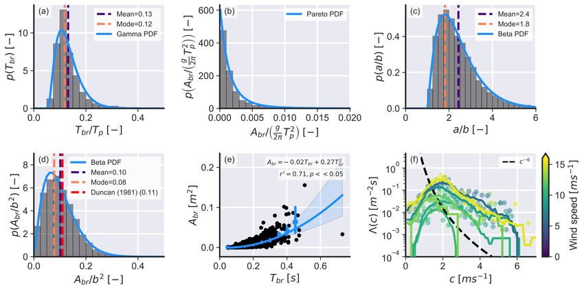
Method

Model Definition

In this study, we have developed a novel method to detect active wave breaking in video imagery data.
Similarly to previous studies, we exploit the fact that breaking wave crests generate characteristic white
foam patches from bubble entrainment30, 31 . Differently from the vast majority of previous methods, here
we make a clear distinction between active wave breaking (that is, visible foam being actively generated
by wave breaking) from passive foam and to all other non-wave breaking instances. To the authors’
knowledge, only the methods of Mironov & Dulov30 and Kleiss & Melville32 have previously attempted
to distinguish between active wave breaking and passive foam. Both their methods start similarly to
ours (see next paragraph) by identifying bright pixels in a given series of images via thresholding. Next,
interconnected pixels are connected in space and time using a nearest neighbor search (Mironov & Dulov30 )
or by extracting connected contours (Kleiss & Melville32 ). In both previous methods, the separation
between active and passive wave breaking is then done by empirically defining foam expansion direction
and velocity limits. The present method aims to remove empirical steps in active wave breaking detection
by using data-driven methods and deep neural networks instead of experiment-specific parameters.

   Our method starts by naïvely identifying wave breaking candidates in a given input image. This was
done by identifying bright (that is, white) pixels in the image using the local thresholding algorithm
available from the OpenCV 33 library with its default parameters. Interconnected regions of bright pixels
in the image were then clustered using DBSCAN34 and a minimum enclosing ellipse35 was fitted to
each identified cluster. The DBSCAN step requires the user to define a minimum number of pixels
to be clustered (default value is 10 for all data used here) and a maximum distance allowed between
pixels (default value of 5 for all data used here). This step resulted in large quantities of bright pixel
patches being detected. At this stage, it was not possible to determine whether a given identified cluster
of pixels represented active wave breaking, passive foam, or any other instance of bright pixels (for
example, birds, boats, coastal structures, sun glints or white clouds). Generically, this step can be thought
of a feature extraction step and can be replaced by any other equivalent approach (for example, image
feature extractors). To avoid exponential memory consumption growth generated by DBSCAN, the input

                                                                                                        4/25
image may be subdivided into blocks of regular size. This step was easily parallelized with performance
increasing linearly with number of computing threads.

   The second step of the method consisted of training a deep convolutional neural network to distinguish
between active wave breaking and passive foam (and all other non-desired occurrences). This step can
be understood as a binary classification step. Figure 1 shows a schematic representation of the present
method. From the original images, randomly selected subsets of size 256x256 pixels centered on the
fitted ellipses were extracted and manually labelled as either active wave breaking (label 1, or positive)
or otherwise (label 0, or negative). The present training dataset was generated using raw video imagery
data from Guimaraẽs et al.36 and consisted of 19000 training and 1300 testing images (see Table 1). The
training dataset is further split into 80% training and 20% validation data37 . The validation dataset is
reserved for future hyper-parameter fine-tuning. Note that the present dataset has a class imbalance of
≈90% towards the negative label, that is, for each active wave breaking sample (label 1, or positive) there
are nine instances that were not active wave breaking (label 0, or negative). Data augmentation38 (rotation,
vertical and horizontal flips, and zoom) was employed during training to increase the variety of samples of
the positive label.

   Five state-of-the-art neural network architectures, or backbones (VGG1639 , ResNet50V240 , Incep-
tionResNetV241 , MobileNetV242 and EfficientNetB543 ), were implemented and can be chosen by end
users (see our Github code repository https://github.com/caiostringari/deepwaves for
usage guidance). All of these backbones make use of convolutional layers to gradually extract information
from the input images. The main differences between them are how many layers they have, the size of the
convolution windows, how data is normalized in each layer and how each layer connects to each other (or
to previous layers in the stack). For example, VGG16 is 16 layers deep, uses 3x3 convolution windows
and has no normalization. InceptionResNetV2 is 164 layers deep, uses a mix of 5x5, 3x3 and 1x1 convolu-
tion windows and uses batch normalization44 to help avoiding overfitting. Residual Networks (namely,
ResNet50V2) not only connect adjacent layers but also take into account errors (residuals) from previous
layers. In general, more modern architectures (namely, EfficientNet) are wider (mainly by having parallel
convolution windows) as well as much deeper than older architectures (namely, VGG16). The final top
layers of the network were fixed for all backbones and consisted of flattening the last convolutional layer,

                                                                                                       5/25
two fully-connected layers with 50% dropout45 , and a final classification layer with sigmoid activation.
The optimization step (training) was done using the Adam46 implementation of the stochastic gradient
descent method47 and binary cross-entropy was used as the loss function. Note that this step must be
computed using a graphics processing unit (GPU) in order to achieve feasible computation times. The
models took from three (VGG16) to twelve (EffientNetB5) hours to train using a NVIDIA GTX 1080
GPU with a batch size of sixty-four images. After the neural networks were sufficiently trained, the best
performing network (VGG16, see below) was used to classify all the naïvely identified wave breaking
candidates and only the events classified as active wave breaking were kept for further analyses. Although
VGG16 was chosen for presenting the results, the performance of the other architectures is nearly identical
to VGG16 on real-world applications. Finally, note that user-tunable parameters for the neural networks
(for example, learning rate and neuron activation thresholds) were kept unchanged from their default
values in the TensorFlow library48 . This implicates that more aggressive parameter optimization could
improve the results presented here even further. For sake of brevity, we refer the reader to the project’s
code repository for guidance on how to select hyper-parameters.
Table 1. Data characterization summary table. f is the sampling frequency in Hertz, D is the duration of
the experiment in seconds, Hs is the significant wave height computed from the wave spectrum, Tp1 and
Tp2 are, respectively, the peak wave period of the first and second spectral partitions computed following
Hanson & Jensen50 , D p is the peak wave direction, and U10 is the wind speed measured or converted
(denoted by the ∗) to a height of 10m above the sea surface using Large & Pond’s51 formula. Tr. S. and Ts.
S. are the sample size of the train and test datasets, respectively.
Location Date and Time f [Hz] D. [min] Hs [m] Tp1 [s] Tp2 [s] U10 [ms−1 ] Dp Tr. S. Ts. S.
Black Sea 2011/10/01 14:18 12 07 0.3 6.20 3.10 10.7* WSW 1000 100
Black Sea 2011/10/04 09:38 12 20 0.36 6.10 2.63 10.1* WSW 1000 100
Black Sea 2011/10/04 11:07 12 30 0.45 6.10 3.16 12.2* WSW 1000 100
Black Sea 2011/10/04 13:30 12 30 0.55 6.60 3.71 12.9* WSW 1000 100
Black Sea 2013/09/22 13:00 10 15 0.66 4.30 30 8.7* E 1000 100
Black Sea 2013/09/25 12:15 12 15 0.41 4.10 1.20 6.1* N 1000 100
Black Sea 2013/09/30 10:20 12 15 0.65 5.70 1.80 15.2* N 1000 100
Adriatic Sea 2014/03/27 09:10 12 60 1.36 5.02 - 9.9 ENE 2000 100
Adriatic Sea 2015/03/05 10:35 12 60 1.33 6.10 5.02 9.0 ENE 2000 100
Yellow Sea 2017/05/13 05:00 10 05 1.93 5.20 4.02 13.4 NW 2000 100
La Jument 2017/12/15 14:20 10 30 5.88 10.00 6.80 13.3 W 2000 100
La Jument 2018/01/03 09:39 10 30 10.03 12.80 9.30 17.9 W 2000 100
La Jument 2018/01/04 11:43 10 30 7.52 11.10 - 14.7 W 2000 100
Total: 19000 1300
The last step of the method consisted of grouping the active wave breaking events in space and time
6/25Figure 1. Schematic representation of a deep convolutional neural network. The input layer consists of
an active wave breaking candidate and has shape 256x256x3 (image height, image width and number of
RGB channels). In the case of a grey-scale image, the single grey channel was triplicated. The red dashed
rectangle in the analyzed image shows the region of interest which, in this particular case, was equal to the
stereo video reconstruction area. The intermediary convolutional layers (or backbones) are
interchangeable with different options available (see text for details). The function of the convolutional
layers is to extract features from the input image by using convolutions (3x3 in this example) and max
pooling49 (that is, selecting the brightest pixel in a given window). The last convolutional layer is flattened
(that is, turned into a one-dimensional vector) and is connected to two fully-connected (that is, multi-layer
perceptron-like) layers and one final classification layer. A 50% dropout (that is, random selection of
neurons in a layer) is applied after each fully connected layer. The final classification layer has one unit
and uses sigmoid activation with a threshold of 0.5.
7/25(note that at this stage bright pixels are only grouped in space). Time-discrete wave breaking events
had their bounding ellipse region filled in pixel space (i, j) and were stacked in time (t) resulting in a
point-cloud-like three-dimensional (i, j,t) structure. The DBSCAN34 algorithm was then used to cluster
these data and obtain uniquely labelled clusters. The two parameters for the DBSCAN algorithm, that is,
the minimum number of samples in each cluster (nmin ) and the minimum distance allowed between two
samples (eps), were set to be equals to the minimum number of points inside a fitted ellipse among all
ellipses (nmin ) and equals to the sampling frequency in Hertz (eps). These values for nmin and eps were
constant among the analyzed datasets. Note that this final step can be replaced by any other density-based
clustering algorithm or other more sophisticated algorithms such as SORT52 (which is also available on
the project’s code repository but not was used here).
Note that up to the clustering step, all calculations were done in pixel domain and "time" was obtained
from sequential frame numbers. To convert between pixel and metric coordinates, the grids constructed
using the stereo-video dataset available from Guimarães et al.36 were used in the present study. If stereo
video data are not available, such conversions could be done knowing the camera position in real-world
(that is, metric) coordinates, which is usually done using surveyed ground control points53, 54 . Conversion
from sequential frame numbers to time (in seconds) can be done by knowing the sample rate (in frames
per second, that is, Hertz) for the data. The total amount of computational time required to process 20
minutes of raw video recorded at 10Hz with an image size of 5 megapixels is approximately two hours
on a modern six-core computer (assuming that a pre-trained neural network is available). Much shorter
processing times are achievable for smaller images sizes and higher number of computation threads.
Evaluation Metrics
Due to the imbalanced characteristic of the dataset, the classification accuracy score in isolation is not
an appropriated metric to evaluated the present test dataset. For instance, a classifier that guesses that all
labels are negative (that is, 0) would automatically obtain a high score (≈ 90%). To properly assess the
performance of the classifier, more robust metrics were defined. These metrics are defined as follows:
• True Positives (T F) and True Negatives (T N) are samples that were correctly classified. False
Positives (FP) or Type I errors are false samples that were incorrectly classified as true, and False
8/25Negatives (FN) or Type II errors are true samples that were classified as false.
• Accuracy is the percentage of examples correctly classified considering both classes, that is,
Accuracy= T TP+T N
+N , where T and N are the total number of positive and negative samples, re-
spectively.
TP
• Precision is the percentage of predicted positives that were correctly classified, that is, Precision= T P+FP .
TP
• Recall is the percentage of actual positives that were correctly classified, that is, Recall= T P+FN
• Area under the curve (AUC) is the area defined by plotting the FP rate against the TP rate (also
referred to as receiver operating characteristic curve). This metric indicates the probability of a
classifier ranking a random positive sample higher than a random negative sample.
All metrics described above were monitored during the training process and were individually assessed to
rank model performance. The training curves shown in Figure 2-a were used to assess when overfitting,
that is, decreases in the loss function value for the training dataset that were not reflected in the validation
dataset, started to occur. Training epochs after overfitting started were discarded. Here we favor the AUC
curves as shown in Figure 2-b to indicate better performing models because AUC is a more robust metric
than the classification score and at the same time presents a smooth evolution with training epochs. Finally,
a confusion matrix (or table of confusion) as shown in Figure 2-c was plotted for each model to assess
Type I and Type II errors.
Results
Classifier performance
From the analysis of all training curves, confusion matrices, and from Table 2, the best performing
backbone architecture during training was ResNet50V2 by a considerable margin (AUC=0.989). These
results however, did not translate to the validation dataset (AUC=0.873). Considering only the validation
data, VGG16 was the best performing backbone with AUC=0.946. Considering only the test dataset,
the best performing model was also VGG16 (AUC=0.855). Overall, VGG16 was selected as the best
performing model and the results presented in the next sections will use this backbone. Other evaluation
9/25metrics such as the accuracy score, precision, and recall closely followed the evolution of AUC with
training epochs (compare Figures 2-a and b, for example). In general, as the loss value decreased, the
number of false positives decreased, which made the precision and recall to increase. This behavior
was consistent for all models. Given that different architectures may perform better for other datasets
and further optimization could change the model ranking presented here, all pre-trained models and
their training metrics evolution are made available in the project’s code repository. Finally, it is worth
mentioning that larger models (for example, VGG19, ResNET152 and EfficientNetB7) could achieve
better results but this was not attempted there due to hardware limitations (that is, these models required
more memory than what was available on the NVIDIA GTX 1080 GPU used in this study).
Figure 2. Examples of training curves and confusion matrix for the best overall performing model
(VGG16). a) Loss function value for training and validation data. b) AUC value for training and validation
data. In a) and b) the hatched area indicates the epochs after which the model started to overfit, the thick
colored lines show smoothed loss or AUC values (average at every 10 epochs), and the transparent lines
show raw loss or AUC values. c) confusion matrix calculated using test data only.
Test Case with Real-world Data
Figure 3 shows the results of the application of the best performing model architecture (VGG16) on La
Jument (2018/01/03 09:39) and Black Sea (2011/10/04 09:38) data. Visual inspection of these results
confirmed the ability of the neural network to correctly classify the naïvely identified wave breaking
candidates and only keep instances that represented active wave breaking. Moreover, the same neural
network was able to correctly classify active wave breaking events for the rogue waves seen at La Jument29
and for the small wind-generated breakers seen in the Black Sea data. This result highlights the ability
10/25Table 2. Evaluation metrics for all tested backbone architectures. Refer to the main manuscript text for
definition of evaluation metrics. The best performing models are shown in boldface. Results are sorted by
AUC.
Model Accuracy TP FP TN FN Precision Recall AUC
Train
ResNetV250 0.97 1414 198 13978 280 0.877 0.835 0.989
VGG16 0.93 855 273 13911 831 0.758 0.507 0.943
InceptionResnetV2 0.927 886 359 13823 802 0.712 0.525 0.932
EfficientNetB5 0.772 1403 3346 10920 297 0.295 0.825 0.874
MobileNet 0.904 436 268 13916 1250 0.619 0.259 0.848
Validation
VGG16 0.932 221 65 3478 204 0.773 0.52 0.946
InceptionResnetV2 0.921 190 81 3466 231 0.701 0.451 0.93
EfficientNetB5 0.809 353 687 2856 72 0.339 0.831 0.897
MobileNet 0.908 123 64 3479 302 0.658 0.289 0.878
ResNetV250 0.919 197 97 3450 224 0.67 0.468 0.873
Test
VGG16 0.876 106 80 945 69 0.57 0.606 0.855
ResNetV250 0.881 95 63 962 80 0.601 0.543 0.843
InceptionResnetV2 0.882 91 57 968 84 0.615 0.52 0.839
EfficientNetB5 0.873 88 65 960 87 0.575 0.503 0.827
MobileNet 0.875 30 5 1020 145 0.857 0.171 0.768
of the neural network to generalize well on the dataset, which is a difficult result to achieve. From the
analysis of the training curves, the averaged classification error (accounting for the imbalance in the
data) should be of the order of ≈10%, which to the authors’ knowledge it was not assessed by other
wave breaking detection methods. We strongly recommend that future research should report active wave
breaking detection errors when used to assess or further develop models that depend on wave breaking
data.
Comparison with Mironov & Dulov (2008)
To highlight the improvements obtained by the present method, this section presents a comparison between
Mironov & Dulov’s (2008)30 automatic active wave breaking detection method and the present method. To
perform this task, data from the 2013 Black Sea experiments in Table 1 that had previously been classified
and investigated in detail by Guimarães55 were used. All the active breaking events (that is, considering
11/25Figure 3. Example of the application of the method. a) Results of the naïve wave breaking detection
(thresholding + DBSCAN) for La Jument data (03/01/2018 09:39). Note the great amount of passive foam
being detected as active wave breaking. b) Results of active wave breaking detection using VGG16 as
backbone for La Jument data (03/01/2018 09:39). Note the significant reduction in the amount of passive
foam being detected. In both plots, number of clusters refers to the number of clusters identified by
DBSCAN. The red dashed rectangle indicates the region of interest which, in these examples, was the
same as the stereo-video reconstruction area. c) Results of the naïve wave breaking detection
(thresholding + DBSCAN) for Black sea data (04/10/2011 09:38). d) Results of active wave breaking
detection using VGG16 as backbone for Black Sea data (04/10/2011 09:38). Animations of these results
are available at https://github.com/caiostringari/deepwaves. In this particular
example, the image was subdivided into blocks of 256x256 pixels for processing. Note that identical
results were seen using other architectures other than VGG16 to classify these data.
12/25all 900s of data) detected using Mironov & Dulov’s (2008)30 were manually classified as true or false
and compared to the labels predicted by our method. To the authors’ knowledge, these data are the only
currently available data that has been classified by both methods as well as manually. Figure 4 shows the
result of the compassion between models. On average, our method has relatively ≈50% less error then
Mironov & Dulov’s (2008) method with an averaged absolute reduction in error of ≈15%. The results in
Figure 4 are also consistent with the results seen in Table 2 which showed that our model had errors in
the order of ≈15% when considering the validation and test datasets. Note that all tested neural network
architectures performed very similarly with only a slight advantage for InceptionResnetV2. It is also worth
mentioning that Mironov & Dulov’s (2008) method was designed and optimized to work specifically with
data from the Black Sea and it is not guaranteed that it will generalize to other datasets. Our method, on
the contrary, has been shown to generalize well for very distinct datasets (see Figure 3, for example) and
with further optimization could achieve even better performance.
Figure 4. Comparison between averaged classification error for active wave breaking detection between
Mironov & Dulov’s (2008)30 method and all the neural network architectures implemented here. The
error bars represent one standard deviation from the mean. The data used for this comparison are from the
2013 Black Sea experiments described in Table 1.
13/25Wave Breaking Statistics
In this section we briefly present examples of wave breaking statistics that can be directly derived from
the classified wave breaking data. For brevity, the analysis is limited to data from the Black Sea because
our classifier performed best at this location (classification errors < 10% considering both 2011 and 2013
experiments). Five quantities will be analysed: the wave breaking duration (Tbr ), the wave breaking area
(Abr ), the major (a) and minor (b) axis of the fitted ellipses (representative of the wave breaking lengths
at their maximum during the active part of the wave breaking), and Phillips’ distribution Λ(c)dc. These
quantities were obtained directly from space-time clustered wave breaking events with the exception of
the cumulative wave breaking area (Abr ) which was calculated from the projections of pixels clustered in
the first step of the method to metric coordinates. The results of this analyses are shown in Figure 5.
The wave breaking duration (Tbr normalized by wave peak period (Tp ), Figure 5-a) roughly followed
a shifted Gamma probability density function (PDF) and had a mean value of 0.12 and most frequent
value (mode) of 0.13. This result shows that the active part of the wave breaking process happens very
quickly. The wave breaking area (Abr , Figure 5-b) closely followed a Pareto distribution which indicates
that large wave breaking events are relatively rare in the data. The ratio between the major and minor axis
of the fitted ellipses (a/b, Figure 5-c) followed a Beta PDF and had a mean of 2.5 and mode of 1.9, which
indicates that the ellipses’ major axis is approximately double the size of the minor axis. Assuming a
negligible wave front angle, the wave breaking area scaling relation from Duncan56 (Abr /b2 , Figure 5-d)
also followed a Beta PDF and had mean of 0.1 and mode of 0.8, which is consistent with the previously
reported value56 (0.1±0.01). The wave breaking area (Figure 5-e) showed a quadratic increase with wave
breaking event duration, which is trivial but seems not to have been previously directly shown before.
Finally, Figure 5-f shows the Λ(c)dc distributions obtained using our method and considering that the
ellipse major axis is representative of the wave breaking length. The observed distributions greatly deviated
from the theoretical c−6 relation12 . Note that all PDF fits shown here were statistically significant at the
95% confidence level using the two-tailed Kolmogorov–Smirnov test. See Table 3 for the description of
the parameters of the PDFs presented in this section and the Discussion section for the contextualization
of these results and the possible implications that they have for future research.
14/25Figure 5. Examples of statistical properties of breaking waves that can be directly obtained from the
proposed method. a) Probability distribution of the wave breaking duration (Tbr ) normalized by wave peak
period (Tp ). The blue line shows the Gamma fit to the data, the purple dashed line shows the mean value
(0.13) and the orange dashed line shows the mode value (0.12). b) Probability distribution of the wave
g 2
breaking area (Abr ) normalized by wavelength ( 2π Tp ). The blue line shows the Pareto fit to the data. c)
Probability distribution of the ratio between major and minor axis (a/b). The blue line shows the Beta fit
to the data, the purple dashed line shows the mean value (2.4) and the orange dashed line shows the mode
value (1.8). d) Probability distribution of the wave breaking area scaling parameter (Abr /b2 ). The blue
line shows the Beta fit to the data, the purple dashed line shows the mean value (0.1), the orange dashed
line shows the mode value (0.08), and the red line shows Duncan’s constant value (0.11). e) Evolution of
the wave breaking area over time. The black markers show the observed values, the error bars show values
binned at 0.15s intervals, the blue line shows the quadratic regression to the data, the blue swath shows the
95% confidence interval for the regression, and r2 is the correlation coefficient. f) Phillips12 Λ(c)dc
distributions assuming that the wave breaking speed is the same as the phase speed of the carrier wave
(that is, c = cbr ) grouped by wind speed. The black dashed line shows the c−6 theoretical decay, the
colored markers show the average crest length binned at 0.1ms−1 wave speed intervals, and the colored
lines show a running average with a window size of 10 bins.
15/25Table 3. Fitted parameters for the distributions seen in Figure 5 . All fits were done using Scipy57 and,
consequently, the values reported here follow Scipy’s conventions.
Distribution Parameter 1 Parameter 2 Location Scale
Figure 5-a Gamma 3.001 - 0.053 0.0260
Figure 5-b Pareto 4.339 - -0.007 0.007
Figure 5-c Beta 6.117 73.948 0.207 30.440
Figure 5-d Beta 6.389 40.470 -0.760 24.438
Discussion
We have presented a new method to detect active wave breaking in video imagery data that is robust
and easily transferable to future studies. Overall, VGG16 was the best performing architecture which
is a surprising result given that VGG is a considerably older architecture that has been superseded by
more recent architectures such as ResNets and EfficientNets43 . Also surprisingly, EfficientNet was one of
the worst performers considering the test dataset despite the state-of-the-art results that this architecture
achieved in recent years43 . One explanation could be that given VGG16 is the model with the highest
number of parameters (despite being the shallowest network), it adapted better to the characteristics of
the present dataset. Another explanation could be that EfficientNet is currently overfit on the ImageNet58
dataset that was used to train this network hence its high reported classification scores. Another aspect
to take into consideration is the speed in which the models can predict on new data (inference). While
VGG16 was the best performing model, its size slows down inference time. In this regard, MobileNetV2
offers real-time inference speed at 10Hz for small image sizes (for example 512 × 512px). Consequently,
a model based on MobileNetV2 could be used to detect active wave breaking in an operational fashion in,
for example, offshore floating wind turbines that are susceptible to wave breaking impacts and used to
adjust anchor and cable settings in real-time.
From the analysis of the application of the method on real-world data, it was visually observed that
small active wave breaking events were not always detected, particularly for the Black Sea data. There
are two possible explanations for this error. The simplest explanation could be that this type of events
is under-represented in the training dataset. The solution for this issue consists of adding more data
representative of these instances to the training dataset. The second possibility is that the image size
16/25becomes too small in the deeper layers of the network which makes it impossible for the network to learn
these events (see below for further discussion). A solution for this issue could be to increase the input
image size but this was not attempted here due to hardware constraints (that is, memory limitation, as
discussed above).
Neural networks have been historically seen as black boxes in which only the final classification
outputs are relevant. There has been, however, an increase in interest to understanding how neural
networks are learning. One technique that is of particular interest for the present paper is the concept of
Gradient-weighted Class Activation Mapping (Grad-CAM)59 . Briefly, this technique shows which regions
of a convolutional layer are more important for the results obtained by the classifier. Figure 6 shows the
results of Grad-CAM applied to examples for all unique locations from Table 1 considering VGG16’s
last convolutional layer. When considering only actively breaking waves (Figure 6-a to d) it is evident
that VGG16 closely mimicked how a human would classify these data, that is, it directly searched for the
regions of the image that corresponded to active wave breaking. In the case of passive foam (Figure 6-e
to h), VGG16 seemed to use larger portions of the image but at the same time focused on the flocculent
foam seen in the images as a human classifier would do. In general, these results show that our model
truly learned how to classify the images and is not merely guessing the labels.
The promising results presented here indicate that the current method should be extended to an
object detection framework. Such a framework would eliminate the need for the image thresholding
and DBSCAN steps. This implementation could be done by using a strongly-supervised architecture
such as UNet60 , or by using a weakly-supervised method derived from Grad-CAM, for example. As a
final recommendation regarding the machine learning aspect of this paper, we strongly encourage future
researchers to add samples to the training dataset that matches their specific research needs instead of
blindly applying the provided pre-trained models.
We have also presented examples of wave breaking statistics that can be obtained using the proposed
method. In general, the patterns observed here agreed with previously reported scaling factors that
support the idea of wave breaking self-similarity. For example, Figure 5-f directly showed that the scaling
parameter Abr /b2 approaches the constant 0.1 value from Duncan’s56 laboratory experiments. Another
variable that showed signs of a self-similar behavior was the wave breaking area (Abr ) which was very well
17/25Figure 6. Results of Grad-CAM59 for all unique experiment locations described in Table 1 applied to
actively breaking waves (top row) and to passive foam (bottom row). a) Actively breaking wave example
recorded at Adriatic Sea (2015/03/05 10:35). b) Actively breaking wave example recorded at the Black
Sea (2011/10/04 11:07). c) Actively breaking wave example recorded at La Jument (2018/01/03 09:39). d)
Actively breaking wave example recorded at the Yellow Sea (2017/05/13 05:00). e) Passive foam example
recorded at Adriatic Sea (2015/03/05 10:35). f) Passive foam example recorded at the Black Sea
(2011/10/04 11:07). g) Passive foam example recorded at La Jument (2018/01/03 09:39). h) Passive foam
example recorded at the (2017/05/13 05:00). In all panels, the color scale indicates the weights of the
class activation map with brighter colors showing regions of the image which the neural network used to
classify each particular sample.
described by a Pareto distribution and presented a steady quadratic increase with wave breaking duration
(Tbr ). Extensive research11, 15 has been grounded on the assumption that wave breaking is self-similar, but
inconsistencies with this approach have been reported before14 . Contrarily to other studies11, 31 , however,
the Λ(c) distributions obtained here did not closely match the theoretical c−6 for a sea-state in equilibrium.
As reported before13 , these differences may be due to the fact that here we only considered actively
breaking waves for our analysis whereas other studies seem to track the speeds of both actively breaking
waves and passive foam31, 32 . Another possibility is that other phenomena not accounted by Phillips’12
theory (for example, wave modulation61 ) play important role on wave breaking. A future publication that
investigates the mechanisms related to the wave breaking kinematics using the method and data obtained
18/25here will soon follow.
Conclusion
We described a novel method to detect and classify actively breaking waves in video imagery data. Our
method achieved promising results when assessed using several different metrics. Further, by analyzing
the deeper layers of our neural network, we showed that the model mimicked how a human classifier
would perform a similar classification task. As an application of the method, we presented wave breaking
statistics and breaking wave crest length distributions. Our method can thus be useful for the investigation
of several ocean-atmosphere interaction processes and should, in the future, lead to advancements in
operational wave forecast models, gas-exchange models, and general safety at seas. Finally, we strongly
recommend that future research should focus on standardized methods to study wave breaking so that a
consistent dataset can be generated and used freely and unambiguously by the community.
References
1. Battjes, J. A. & Janssen, J. Energy loss and set-up due to breaking of random waves. Coast. Eng. 32,
569–587 (1978).
2. Thornton, E. B. & Guza, R. T. Transformation of Wave Height Distribution. J. Geophys. Res. 88,
5925–5938 (1983).
3. Banner, M. L., Babanin, A. V. & Young, I. R. Breaking Probability for Dominant Waves on
the Sea Surface. J. Phys. Oceanogr. 30, 3145–3160, DOI: 10.1175/1520-0485(2000)0302.0.CO;2 (2000).
4. Banner, M. L., Gemmrich, J. R. & Farmer, D. M. Multiscale measurements of ocean wave break-
ing probability. J. Phys. Oceanogr. 32, 3364–3375, DOI: 10.1175/1520-0485(2002)0322.0.CO;2 (2002).
5. Cavaleri, B. Y. L. Wave Modeling: Where to Go in the Future. Bull. Am. Meteorol. Soc. 207–2014,
DOI: 10.1175/BAMS-87-2-207 (2006).
19/256. The WAVEWATCH Development Group (WW3DG). User manual and system documentation of
WAVEWATCH III R version 6.07. Tech. Rep., NOAA/NWS/NCEP/MMAB, College Park, MD, USA
(2019).
7. Booij, N., Ris, R. C. & Holthuijsen, L. H. A third-generation wave model for coastal regions 1 .
Model description and validation. J. Geophys. Res. 104, 7649–7666 (1999).
8. The WANDI Group. The WAN Model - A Third Generation Ocean Wave Prediction Model. J. Phys.
Oceanogr. 18, 1775–1810 (1988).
9. Filipot, J. F., Ardhuin, F. & Babanin, A. V. A unified deep-to-shallow water wave-breaking probability
parameterization. J. Geophys. Res. Ocean. 115, 1–15, DOI: 10.1029/2009JC005448 (2010).
10. Stringari, C. E. & Power, H. E. The Fraction of Broken Waves in Natural Surf Zones. J. Geophys.
Res. Ocean. 124, 1–27, DOI: 10.1029/2019JC015213 (2019). arXiv:1904.06821v1.
11. Melville, W. K. & Matusov, P. Distribution of breaking waves at the ocean surface. Nature 417,
58–63, DOI: 10.1038/417058a (2002).
12. Phillips, O. M. Spectral and statistical properties of the equilibrium range in wind-generated gravity
waves. J. Fluid Mech. 156, 505–531, DOI: 10.1017/S0022112085002221 (1985).
13. Banner, M. L., Zappa, C. J. & Gemmrich, J. R. A note on the Phillips spectral framework for ocean
whitecaps. J. Phys. Oceanogr. 44, 1727–1734, DOI: 10.1175/JPO-D-13-0126.1 (2014).
14. Gemmrich, J. R., Banner, M. L. & Garrett, C. Spectrally resolved energy dissipation rate and
momentum flux of breaking waves. J. Phys. Oceanogr. 38, 1296–1312, DOI: 10.1175/2007JPO3762.1
(2008).
15. Romero, L. Distribution of Surface Wave Breaking Fronts. Geophys. Res. Lett. 46, 10463–10474,
DOI: 10.1029/2019GL083408 (2019).
16. Yurovsky, Y. Y., Kudryavtsev, V. N., Chapron, B. & Grodsky, S. A. Modulation of Ka-Band Doppler
Radar Signals Backscattered from the Sea Surface. IEEE Transactions on Geosci. Remote. Sens. 56,
2931–2948, DOI: 10.1109/TGRS.2017.2787459 (2018).
20/2517. Huang, L., Liu, B., Li, X., Zhang, Z. & Yu, W. Technical evaluation of Sentinel-1 IW mode cross-pol
radar backscattering from the ocean surface in moderate wind condition. Remote. Sens. 9, 1–21, DOI:
10.3390/rs9080854 (2017).
18. Hwang, P. A., Zhang, B., Toporkov, J. V. & Perrie, W. Comparison of composite Bragg theory and
quad-polarization radar backscatter from RADARSAT-2: With applications to wave breaking and
high wind retrieval. J. Geophys. Res. Ocean. 115, 1–12, DOI: 10.1029/2009JC005995 (2010).
19. Monahan, E. C. Oceanic whitecaps: Sea surface features detectable via satellite that are indicators of
the magnitude of the air-sea gas transfer coefficient. J. Earth Syst. Sci. 111, DOI: 10.1007/BF02701977
(2002).
20. Reul, N. & Chapron, B. A model of sea-foam thickness distribution for passive microwave remote
sensing applications. J. Geophys. Res. C: Ocean. 108, 19–1, DOI: 10.1029/2003jc001887 (2003).
21. Carini, R. J., Chickadel, C. C., Jessup, A. T. & Thompson, J. Estimating wave energy dissipation
in the surf zone using thermal infrared imagery. J. Geophys. Res. Ocean. 120, 3937–3957, DOI:
10.1002/2014JC010561.Received (2015).
22. Wang, S. et al. Improving the Upper-Ocean Temperature in an Ocean Climate Model (FESOM 1.4):
Shortwave Penetration Versus Mixing Induced by Nonbreaking Surface Waves. J. Adv. Model. Earth
Syst. 11, 545–557, DOI: 10.1029/2018MS001494 (2019).
23. Komori, S. et al. Laboratory measurements of heat transfer and drag coefficients at extremely high
wind speeds. J. Phys. Oceanogr. 48, 959–974, DOI: 10.1175/JPO-D-17-0243.1 (2018).
24. Buscombe, D. & Carini, R. J. A data-driven approach to classifying wave breaking in infrared imagery.
Remote. Sens. 11, 1–10, DOI: 10.3390/RS11070859 (2019).
25. Buscombe, D., Carini, R. J., Harrison, S. R., Chickadel, C. C. & Warrick, J. A. Optical wave gauging
using deep neural networks. Coast. Eng. 155, 103593, DOI: 10.1016/j.coastaleng.2019.103593
(2020).
26. Kim, J., Kim, J., Kim, T., Huh, D. & Caires, S. Wave-tracking in the surf zone using coastal video
imagery with deep neural networks. Atmosphere 11, 1–13, DOI: 10.3390/atmos11030304 (2020).
21/2527. Bieman, J. P. D., Ridder, M. P. D. & Gent, M. R. A. V. Deep learning video analysis as measurement
technique in physical models. Coast. Eng. 158, 103689, DOI: 10.1016/j.coastaleng.2020.103689
(2020).
28. Zheng, C. W., Chen, Y. G., Zhan, C. & Wang, Q. Source Tracing of the Swell Energy: A Case Study
of the Pacific Ocean. IEEE Access 7, 139264–139275, DOI: 10.1109/ACCESS.2019.2943903 (2019).
29. Filipot, J.-F. et al. La Jument lighthouse: a real-scale laboratory for the study of giant waves and
their loading on marine structures. Philos. Transactions Royal Soc. A: Math. Phys. Eng. Sci. 377,
20190008, DOI: 10.1098/rsta.2019.0008 (2019).
30. Mironov, A. S. & Dulov, V. A. Detection of wave breaking using sea surface video records. Meas.
Sci. Technol. 19, DOI: 10.1088/0957-0233/19/1/015405 (2008).
31. Sutherland, P. & Melville, W. K. Field measurements and scaling of ocean surface wave-breaking
statistics. Geophys. Res. Lett. 40, 3074–3079, DOI: 10.1002/grl.50584 (2013).
32. Kleiss, J. M. & Melville, W. K. Observations of wave breaking kinematics in fetch-limited seas. J.
Phys. Oceanogr. 40, 2575–2604, DOI: 10.1175/2010JPO4383.1 (2010).
33. Bradski, G. The OpenCV Library. Dr. Dobb’s J. Softw. Tools (2000).
34. Ester, M., Kriegel, H.-P., Sander, J. & Xu, X. Density-Based Clustering Methods. Compr. Chemom.
2, 635–654, DOI: 10.1016/B978-044452701-1.00067-3 (1996). 10.1.1.71.1980.
35. Moshtagh, N. Minimum Volume Enclosing Ellipsoids. Convex Optim. 111, 112–118 (2005).
36. Guimaraes, P. V. et al. A Data Set of Sea Surface Stereo Images to Resolve Space-Time Wave Fields.
Sci. Data 7, 1–12, DOI: 10.12770/af599f42-2770-4d6d-8209-13f40e2c292f (2020).
37. Hastie, T., Tibshirani, R. & Friedman, J. The Elements of Statistical Learning (Springer International
Publishing, 2009), second edi edn.
38. Shorten, C. & Khoshgoftaar, T. M. A survey on Image Data Augmentation for Deep Learning. J. Big
Data 6, DOI: 10.1186/s40537-019-0197-0 (2019).
39. Simonyan, K. & Zisserman, A. Very deep convolutional networks for large-scale image recognition.
3rd Int. Conf. on Learn. Represent. ICLR 2015 - Conf. Track Proc. 1–14 (2015). arXiv:1409.1556v6.
22/2540. He, K., Zhang, X., Ren, S. & Sun, J. Identity mappings in deep residual networks. Lect. Notes
Comput. Sci. (including subseries Lect. Notes Artif. Intell. Lect. Notes Bioinformatics) 9908 LNCS,
630–645, DOI: 10.1007/978-3-319-46493-0_38 (2016). 1603.05027.
41. Szegedy, C., Ioffe, S., Vanhoucke, V. & Alemi, A. A. Inception-v4, inception-ResNet and the impact
of residual connections on learning. 31st AAAI Conf. on Artif. Intell. AAAI 2017 4278–4284 (2017).
1602.07261.
42. Howard, A. G. et al. MobileNets: Efficient Convolutional Neural Networks for Mobile Vision
Applications (2017). 1704.04861.
43. Tan, M. & Le, Q. V. EfficientNet: Rethinking model scaling for convolutional neural networks. 36th
Int. Conf. on Mach. Learn. ICML 2019 2019-June, 10691–10700 (2019). 1905.11946.
44. Ioffe, S. & Szegedy, C. Batch normalization: Accelerating deep network training by reducing internal
covariate shift. 32nd Int. Conf. on Mach. Learn. ICML 2015 1, 448–456 (2015). 1502.03167.
45. Srivastava, N., Hinton, G., Krizhevsky, A., Sutskever, I. & Salakhutdinov, R. Dropout: A Simple
Way to Prevent Neural Networks from Overfitting. J. Mach. Learn. Res. 15, 1929–1958, DOI:
10.1109/ICAEES.2016.7888100 (2014).
46. Kingma, D. P. & Ba, J. Adam: A Method for Stochastic Optimization. In 3rd International Conference
for Learning Representations, 1–15, DOI: http://doi.acm.org.ezproxy.lib.ucf.edu/10.1145/1830483.
1830503 (San Diego, California, 2014). 1412.6980.
47. Ruder, S. An overview of gradient descent optimization algorithms (2016). 1609.04747.
48. Abadi, M. et al. TensorFlow: Large-scale machine learning on heterogeneous systems (2015).
Software available from tensorflow.org.
49. Nagi, J. et al. Max-Pooling Convolutional Neural Networks for Vision-based Hand Gesture Recogni-
tion. In 2011 IEEE International Conference on Signal and Image Processing Applications, ICSIPA
2011, 342–347 (2011).
50. Hanson, J. L. & Jensen, R. Wave system diagnostics for numerical wave models. 8 th Int. Work. on
Wave Hindcasting Forecast. Oahu, Hawaii, Novemb. (2004).
23/2551. Large, W. G. & Pond, S. Open Ocean Momentum Flux Measurements in Moderate to Strong Winds.
J. Phys. Oceanogr. DOI: 10.1175/1520-0485(1981)0112.0.CO;2 (1981).
52. Bewley, A., Ge, Z., Ott, L., Ramos, F. & Upcroft, B. Simple online and realtime tracking. Proc. - Int.
Conf. on Image Process. ICIP 2016-August, 3464–3468, DOI: 10.1109/ICIP.2016.7533003 (2016).
1602.00763.
53. Holman, R. A. & Stanley, J. The history and technical capabilities of Argus. Coast. Eng. 54, 477–491,
DOI: 10.1016/j.coastaleng.2007.01.003 (2007).
54. Schwendeman, M., Thomson, J. & Gemmrich, J. R. Wave breaking dissipation in a Young Wind Sea.
J. Phys. Oceanogr. 44, 104–127, DOI: 10.1175/JPO-D-12-0237.1 (2014).
55. Guimaraes, P. V. Sea surface and energy dissipation. Ph.D. thesis, Universitè de Bretagne Loire
(2018).
56. Duncan, J. H. An Experimental Investigation of Breaking Waves Produced by a Towed Hydrofoil.
Proc. Royal Soc. A: Math. Phys. Eng. Sci. 377, 331–348, DOI: 10.1098/rspa.1981.0127 (1981).
57. Virtanen, P. et al. SciPy 1.0: Fundamental Algorithms for Scientific Computing in Python. Nat.
Methods DOI: https://doi.org/10.1038/s41592-019-0686-2 (2020).
58. Russakovsky, O. et al. ImageNet Large Scale Visual Recognition Challenge. Int. J. Comput. Vis. 115,
211–252, DOI: 10.1007/s11263-015-0816-y (2015). 1409.0575.
59. Selvaraju, R. R. et al. Grad-CAM: Visual Explanations from Deep Networks via Gradient-Based
Localization. Int. J. Comput. Vis. 128, 336–359, DOI: 10.1007/s11263-019-01228-7 (2020). 1610.
02391.
60. Ronneberger, O., P.Fischer & Brox, T. U-net: Convolutional networks for biomedical image segmen-
tation. In Medical Image Computing and Computer-Assisted Intervention (MICCAI), vol. 9351 of
LNCS, 234–241 (Springer, 2015). (available on arXiv:1505.04597 [cs.CV]).
61. Donelan, M. A., Haus, B. K., Plant, W. J. & Troianowski, O. Modulation of short wind waves by long
waves. J. Geophys. Res. Ocean. 115, 1–12, DOI: 10.1029/2009JC005794 (2010).
24/25Acknowledgements
This work benefited from France Energies Marines and State financing managed by the National Research
Agency under the Investments for the Future program bearing the reference numbers ANR-10-IED-0006-
14 and ANR-10-IEED-0006-26 for the projects DiME and CARAVELE.
Author contributions statement
C.E.S. idealized and implemented the method, C.E.S. drafted the manuscript, P.V.G., F.L., J.F.F. and R. D.
conducted the field experiments, C.E.S. and P.V.G. analyzed the data, J.F. provided funding. All authors
reviewed the manuscript.
Additional information
Data, pre-trained networks and auxiliary programs necessary to reproduce the results in this paper are
available at: https://github.com/caiostringari/deepwaves.
Competing Interests Statement
The authors declare no known competing interests.
25/25You can also read