SCOPE Climate: a 142-year daily high-resolution ensemble meteorological reconstruction dataset over France - Earth System Science Data
←
→
Page content transcription
If your browser does not render page correctly, please read the page content below
Earth Syst. Sci. Data, 11, 241–260, 2019
https://doi.org/10.5194/essd-11-241-2019
© Author(s) 2019. This work is distributed under
the Creative Commons Attribution 4.0 License.

                 SCOPE Climate: a 142-year daily high-resolution
                    ensemble meteorological reconstruction
                             dataset over France
                     Laurie Caillouet1,a , Jean-Philippe Vidal1 , Eric Sauquet1 , Benjamin Graff2 , and
                                                 Jean-Michel Soubeyroux3
         1 Irstea,UR RiverLy, Centre de Lyon-Villeurbanne, 5 rue de la Doua CS 20244, 69625 Villeurbanne, France
                       2 Compagnie Nationale du Rhône (CNR), 2 rue André Bonin, 69004 Lyon, France
                 3 Météo-France, Direction de la Climatologie et des Services Climatiques, 42 avenue Coriolis,

                                               31057 Toulouse Cedex 1, France
       a now at: INRS, Centre Eau Terre Environnement, 490 rue de la Couronne, Québec (Québec) G1K 9A9, Canada

                             Correspondence: Laurie Caillouet (laurie.caillouet@gmail.com)

                                   Received: 10 July 2018 – Discussion started: 2 August 2018
                      Revised: 30 December 2018 – Accepted: 29 January 2019 – Published: 21 February 2019

       Abstract. SCOPE Climate (Spatially COherent Probabilistic Extended Climate dataset) is a 25-member ensem-
       ble of 142-year daily high-resolution reconstructions of precipitation, temperature, and Penman–Monteith refer-
       ence evapotranspiration over France, from 1 January 1871 to 29 December 2012. SCOPE Climate provides an
       ensemble of 25 spatially coherent gridded multivariate time series. It is derived from the statistical downscaling
       of the Twentieth Century Reanalysis (20CR) by the SCOPE method, which is based on the analogue approach.
       SCOPE Climate performs well in comparison to both dependent and independent data for precipitation and tem-
       perature. The ensemble aspect corresponds to the uncertainty related to the SCOPE method. SCOPE Climate
       is the first century-long gridded high-resolution homogeneous dataset available over France and thus has paved
       the way for improving knowledge on specific past meteorological events or for improving knowledge on climate
       variability, since the end of the 19th century. This dataset has also been designed as a forcing dataset for long-
       term hydrological applications and studies of the hydrological consequences of climate variability over France.
       SCOPE Climate is freely available for any non-commercial use and can be downloaded as NetCDF files from
       https://doi.org/10.5281/zenodo.1299760 for precipitation, https://doi.org/10.5281/zenodo.1299712 for tempera-
       ture, and https://doi.org/10.5281/zenodo.1251843 for reference evapotranspiration.

1   Introduction to SCOPE Climate                                 started earlier with a higher density like the UK, long-term
                                                                  gridded datasets of daily rainfall have been derived based on
Historical surface meteorological observations like precipi-      the interpolation between stations from 1890 onwards (Keller
tation and temperature are more and more scarce and sparse        et al., 2015). Similarly, daily gridded estimates of potential
when going back in time to before the 1950s. Even in a data-      evapotranspiration have recently been derived from the net-
rich country like France, the number of available stations in     work of mean monthly temperature observations in the UK
databases is reduced to only a few in the early 1870s. Data       from 1891 onwards (Tanguy et al., 2018).
rescue efforts are ongoing (Jourdain et al., 2015) but the           Two global reanalyses spanning the entire 20th century
present state of databases prevents us performing century-        have recently been released: the Twentieth Century Reanal-
long analyses of climate variability and extremes over large      ysis (20CR, Compo et al., 2011) and the European Reanal-
regions in a both spatially and temporally homogeneous way.       ysis of the Twentieth Century (ERA-20C, Poli et al., 2016).
In some other countries with an observation network that          They provide the opportunity to reconstruct long-term local-

Published by Copernicus Publications.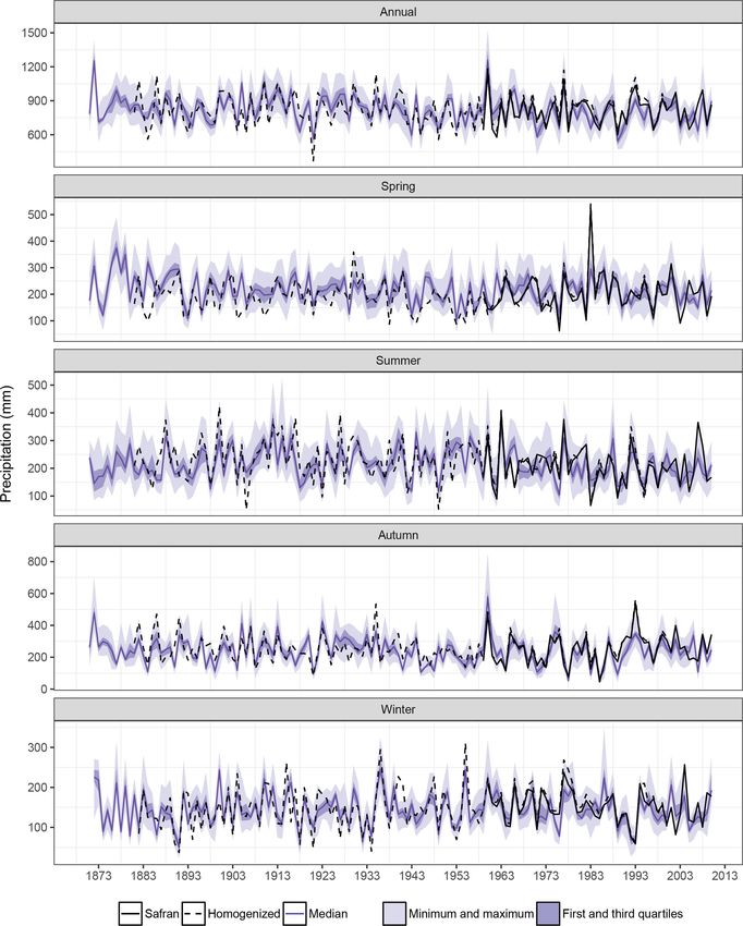
242                                                                                         L. Caillouet et al.: SCOPE Climate

scale meteorological data through downscaling techniques,          2     Statistical downscaling of 20CR with the SCOPE
avoiding the use of non-homogeneous ground observation                   method
networks. Statistical downscaling methods may be used to
derive daily local-scale near-surface meteorological variables     2.1     Data
from synoptic-scale atmospheric variables provided by such
                                                                   2.1.1    Source for local predictands: Safran
global extended reanalyses. 20CR has already been down-
scaled for specific regions in France (e.g. Kuentz et al., 2015)   Safran is the French near-surface reanalysis available on the
or for the entire country (Minvielle et al., 2015; Dayon et al.,   hourly timescale and 8 km spatial resolution, from 1 Au-
2015; Bonnet et al., 2017) but without a locally optimized         gust 1958 onwards (Vidal et al., 2010). Safran was derived
method and/or in a deterministic way, thus preventing any          based on an optimal interpolation between all surface ob-
analyses from focusing on the detailed local outputs and/or        servations available in the Météo-France database and a first
the downscaling uncertainty.                                       guess from the ERA-40 reanalysis (Uppala et al., 2005) until
   Caillouet et al. (2016, 2017) proposed a statistical down-      2002 and from ECMWF operational analyses afterwards for
scaling of 20CR over the period 1871–2012 with an en-              608 climatically homogeneous zones in France (Quintana-
semble method locally optimized over France – based on             Seguí et al., 2008). Daily reference evapotranspiration was
an analogue resampling of the existing 50-year-long Safran         computed based on the hourly Penman–Monteith formula
near-surface reanalysis (Vidal et al., 2010) – in order to im-     (Allen et al., 1998). Vidal et al. (2010) showed that the Safran
prove the knowledge on past hydrometeorological condi-             errors in precipitation are relatively low and constant over the
tions and climate variability, since the end of the 19th cen-      1958–2008 period, while Safran errors in temperature are de-
tury in France. SCOPE Climate (Spatially COherent Prob-            creasing with an increasing number of assimilated surface
abilistic Extended Climate dataset), the resulting dataset, is     observations.
a daily high-resolution ensemble reconstruction of precipi-           Local predictands used to derive SCOPE Climate are grid-
tation, temperature and Penman–Monteith reference evapo-           ded daily precipitation, temperature, and reference evapo-
transpiration fields in France from 1 January 1871 to 29 De-       transpiration over the period 1 August 1958 to 31 July 2008.
cember 2012. Available on a 8 km grid, SCOPE Climate has           More recent Safran data can therefore be used for a com-
the appropriate space and time resolutions for various hy-         pletely independent comparison.
drological applications, such as the study of drought events,
large-scale floods or streamflow variability over the 20th cen-    2.1.2    Source for atmospheric predictors: 20CR
tury; see Caillouet et al. (2017) for an application on re-
constructing historical low-flow events. This paper proposes       The Twentieth Century Reanalysis (20CR) is a large-scale
making SCOPE Climate accessible to the research commu-             reanalysis spanning the entire 20th century and developed
nity.                                                              by the National Oceanic and Atmospheric Administration
   The most generic methodological choices have been made          (NOAA) (Compo et al., 2011). 20CR V2 chosen here only
in the creation of SCOPE Climate to promote the widest             uses 6-hourly surface level pressure (SLP) observations from
possible use of the dataset, e.g. by not favouring precipita-      the International Surface Pressure Databank (ISPD v2.2,
tion over temperature or low extremes over high ones. The          Compo et al., 2010) in the ensemble Kalman filter assimila-
length (142 years), the spatial availability (whole of France)     tion process and the monthly sea surface temperature (SST)
as well as the ensemble aspect (25 members) will enable var-       and sea-ice concentration fields from the Hadley Centre
ious spatio-temporal analyses – such analyses may take ac-         global sea ice and sea surface temperature (HadISST, Rayner
count of the uncertainty in the statistical downscaling step       et al., 2003) as boundary conditions. This choice has been
– to enhance the knowledge of past meteorology and cli-            made to avoid inhomogeneities due to the assimilation of ob-
mate, and their hydrological impacts. SCOPE Climate more-          servations from different systems.
over provides spatially consistent multivariate gridded time          Six atmospheric predictors are considered in the down-
series for each ensemble member, which make it suitable for        scaling process used to derive SCOPE Climate: temperatures
studies requiring both inter-variable and spatial consistency,     at 925 and 600 hPa, geopotential heights at 1000 and 500 hPa,
e.g. catchment-scale hydrology.                                    vertical velocity at 850 hPa, precipitable water content, rel-
   This paper presents the SCOPE Climate dataset, first by         ative humidity at 850 hPa – all from the 6-hourly analysis
introducing the methodological framework developed to de-          – and large-scale 2 m temperature (T2m) from the 6-hourly
rive it in Sect. 2. Characteristics of SCOPE Climate are then      forecast.
detailed in Sect. 3 through examples and validation results.          20CR predictors are available at 2.0◦ spatial resolution
Section describes how to access the dataset, and Sect. 5 con-      and 6-hourly temporal resolution from 1 January 1871 to
siders some of its limitations.                                    31 December 2012. Five predictors – temperature, geopoten-
                                                                   tial height, vertical velocity, precipitable water content, and
                                                                   relative humidity – have been spatially interpolated with a bi-
                                                                   linear interpolation on a 2.5◦ grid for input of the downscal-

Earth Syst. Sci. Data, 11, 241–260, 2019                                            www.earth-syst-sci-data.net/11/241/2019/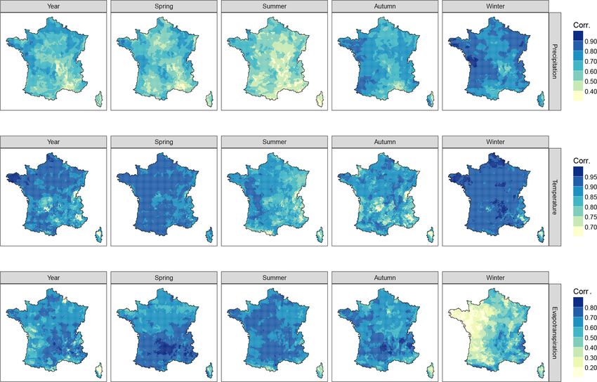
L. Caillouet et al.: SCOPE Climate                                                                                              243

ing method. The ensemble mean of the 56-member ensemble             the entire target period. For a date in the target period, large-
of 20CR was considered for building SCOPE Climate (see              scale predictors are compared to those of all dates over the
Sect. 5).                                                           archive. Dates from the archive period with the most similar
                                                                    predictors are then chosen as analogues. Local-scale predic-
2.1.3    Source for oceanic predictor: ERSST                        tand from the selected analogue dates are taken as an ensem-
                                                                    ble of plausible predictand values for the target date.
The NOAA Extended Reanalysis Sea Surface Temperature                   As SANDHY was initially aimed at quantitative precipi-
(ERSST) version 3b is a global sea surface temperature              tation forecasting, the predictand is daily precipitation. The
(SST) reanalysis and has been available at a 2.0◦ spatial           predictors are used in four analogy levels, i.e. four consecu-
resolution and a monthly temporal resolution since 1 Jan-           tive subsampling steps, optimized by Ben Daoud et al. (2011,
uary 1854 (Smith and Reynolds, 2003; Smith et al., 2008).           2016). The first level selects N analogue days on tempera-
Like 20CR, this version does not use satellite data to avoid        ture at 925 and 600 hPa with the exclusion of a 9-day window
inhomogeneities. Monthly values of SST over the optimised           centred on the target date. N is taken as 100 times the number
grid cell south of Brittany (4◦ W, 46◦ N) over the period           of years in the archive period. The second level selects 170
1871–2012 were extracted and interpolated with splines to           analogues on geopotential heights of 500 and 1000 hPa. The
the daily timescale required by the downscaling process (see        third level selects 70 analogues thanks to an analogy on verti-
Appendix B in Caillouet et al., 2017) and constitutes the sev-      cal velocity at 850 hPa and the final level selects 25 analogues
enth large-scale predictor of the SCOPE method.                     on humidity, which is considered as the product of the pre-
                                                                    cipitable water content and the relative humidity at 850 hPa.
2.2     The SCOPE statistical downscaling method                       The similarity criterion used for the analogy levels on
                                                                    temperature, vertical velocity, and humidity is the Euclidean
The Spatially COherent Probabilistic Extension method               distance, with equal weights when different pressure levels
(SCOPE, Caillouet et al., 2017) is the statistical method used      are used. The analogy on geopotential height is measured
to downscale 20CR and derive the SCOPE Climate dataset.             through the shape similarity between fields with the Teweles
SCOPE is an extension of the Statistical ANalogue Down-             and Wobus (1954) criterion. The predictor domain (spatial
scaling method for HYdrology (SANDHY, Ben Daoud et al.,             domain where the analogy is sought) depends on the Safran
2011, 2016; Radanovics et al., 2013). It can be divided in four     zone considered. The spatial domain for the first, third, and
steps that have been briefly described in the Appendix B of         fourth analogy levels is the closest large-scale grid point to
Caillouet et al. (2017) and that are detailed in the paragraphs     each zone. For the analogy level on geopotential, this domain
below:                                                              had been originally optimized by Radanovics et al. (2013)
                                                                    over the 1 August 1982–31 July 2002 period on the 608 cli-
  – applying the SANDHY method (Sect. 2.2.1),                       matically homogeneous Safran zones covering France using
                                                                    predictors from ERA-40 (Uppala et al., 2005). SCOPE Cli-
  – subselecting SANDHY analogues to reconstruct both
                                                                    mate was produced by re-optimizing the spatial domain fol-
    precipitation and temperature (Sect. 2.2.2),
                                                                    lowing the Radanovics et al. (2013) method, but with 20CR
  – correcting for precipitation bias (Sect. 2.2.3),                predictors. Five near-optimal domains are obtained for each
                                                                    zone in France using an algorithm of growing rectangular
  – ensuring spatial coherence (Sect. 2.2.4).                       domains. The performance criterion for this optimization
                                                                    was the continuous ranked probability score (CRPS, Brown,
2.2.1    Step 1: Applying the SANDHY method
                                                                    1974; Matheson and Winkler, 1976), widely used for proba-
                                                                    bilistic verification forecast. Domains found from neighbour-
The SANDHY method is an ensemble statistical downscal-              ing zones were also considered if they provide a better per-
ing method following an analogue approach. It is based on           formance.
the idea introduced by Lorenz (1969) that similar atmo-                The synthetic diagram in Fig. 1 summarizes the differ-
spheric situations lead to similar local effects. The analogue      ent steps described above. 20CR variables are used as pre-
approach uses two concurrent datasets, a large-scale reanal-        dictors (see Sect. 2.1.2), whereas Safran precipitation is se-
ysis containing predictors and a local-scale meteorological         lected as a predictand (see Sect. 2.1.1). The archive period
dataset containing predictands. SANDHY thus uses two pe-            over which the predictors–predictand relationship is set up is
riods: a target period, over which reconstruction take place,       1 August 1958 to 31 July 2008. The target period considered
and an archive period, from which analogue meteorologi-             is the whole period spanned by 20CR V2 data, i.e. 1 Jan-
cal situations are picked up to reconstruct the target period.      uary 1871 to 31 December 2012. The different downscaling
The two datasets (here 20CR and Safran) have to be avail-           steps are applied 5 times using one of the near-optimal anal-
able throughout the archive period, in which the predictor–         ogy domain for geopotential at each run. The application of
predictand relationship is set up. In this reconstruction set-up,   SANDHY with these settings provides an ensemble of 125
only the large-scale reanalysis (20CR) must be available over       analogue dates for each date in the target period, indepen-

www.earth-syst-sci-data.net/11/241/2019/                                              Earth Syst. Sci. Data, 11, 241–260, 2019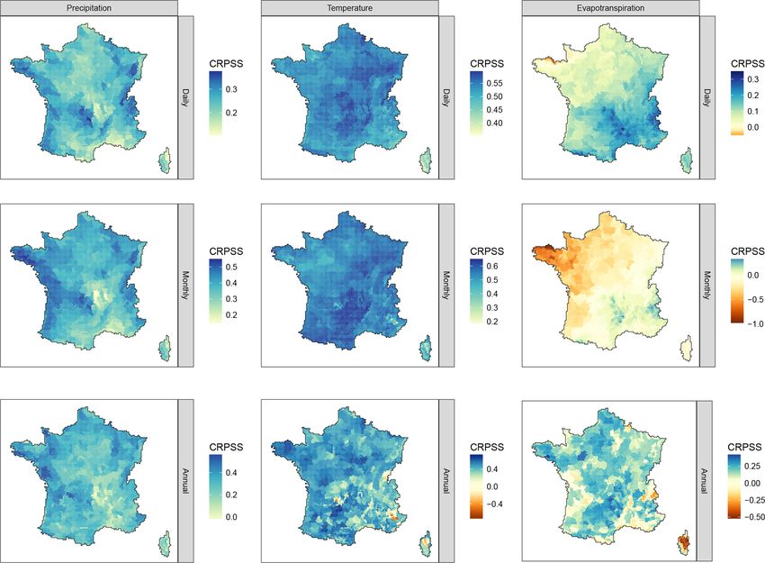
244                                                                                              L. Caillouet et al.: SCOPE Climate

Figure 1. Synthetic diagram showing the sequence of analogy steps in the SANDHY method to reconstruct precipitation and temperature
over a given climatically homogeneous zone and for a specific target date.

dently for the 608 climatically homogeneous zones covering              geneous zones in France is used for computing the analogy
France. Applying SANDHY to each zone leads to no spatial                on SST (optimised at location 4◦ W, 46◦ N). The grid point
consistency between zones, the latter being added with the              for computing the T2m analogy is chosen as the land grid
method presented in Sect. 2.2.4.                                        point closest to each climatically homogeneous zone, follow-
   Analogues dates included in the period 1 August 1958                 ing the approach used for levels 1, 3, and 4 in the standard
to 31 July 2008 are then converted to meteorological vari-              SANDHY method. A detailed validation of results from the
ables by resampling Safran reanalysis data. The analogues               chain SANDHY + stepwise (also called SANDHY-SUB) for
obtained from SANDHY are not only used for precipitation,               temperature and precipitation over France was performed by
but also for temperature and reference evapotranspiration.              Caillouet et al. (2016).

2.2.2   Step 2: Subselecting SANDHY analogues                           2.2.3   Step 3: Correcting for precipitation bias
An overestimation of precipitation in spring and an underes-            A third step consists of a bias correction of SANDHY-SUB
timation of precipitation in autumn was found in SANDHY                 precipitation. Indeed, the median of annual precipitation be-
outputs for zones with high seasonal asymmetry (e.g.,                   tween Safran and the reconstructed precipitation showed a
Mediterranean areas). Moreover, winter and summer tem-                  dry bias of around 10 % (see Caillouet et al., 2016). Instead
peratures were respectively over- and underestimated (Cail-             of applying common bias correction techniques, a correction
louet et al., 2016). This last result was not unexpected since          approach similar to the one adopted by Sippel et al. (2016)
SANDHY predictors were chosen for their strong relation                 has been considered here, keeping a maximum inter-variable
to precipitation and not to temperature. To reduce these bi-            coherence that is inherent to analogue methods.
ases while keeping unchanged the structure of the SANDHY                   For each target date between 1871 and 2012, the N ana-
method, two analogy levels have been applied to the 125 ana-            logues giving the lowest precipitation, including zeros, are
logues dates resulting from the application of SANDHY.                  removed. N analogues are then randomly resampled from
   This method is called stepwise subselection and was de-              the (25 – N) left to keep a 25-member sample size. N is in-
scribed by Caillouet et al. (2016). The first additional analogy        dependently defined for each of the 608 zones in France. It is
level selects 80 analogues out of 125 based on the similarity           defined so that the bias with respect to Safran data (over the
of SST values. The second level selects 25 analogues based              archive period) is minimized and has values ranging from 0
on the similarity of T2m values. The number of analogues at             to 3 across France. By construction, this number increases
each level was optimized by Caillouet et al. (2016). The sim-           with precipitation underestimation. All variables – precip-
ilarity criterion for both levels is the Euclidean distance. For        itation, but also temperature and evapotranspiration – that
the sake of consistency over France and parsimony of param-             correspond to the removed N analogue dates are discarded,
eters, a single grid point common to all climatically homo-             therefore preserving the inter-variable consistency. Impor-

Earth Syst. Sci. Data, 11, 241–260, 2019                                                 www.earth-syst-sci-data.net/11/241/2019/
L. Caillouet et al.: SCOPE Climate                                                                                            245

tantly, this resampling-based correction of precipitation does      consists of an ensemble of 25 equally plausible individual
not affect the temperature bias and interannual correlation         members of multivariate gridded meteorological series. Each
described in Caillouet et al. (2016). This technique allows         member gathers daily gridded times series of precipitation,
one to retrieve a near-zero bias in mean interannual precipi-       temperature, and reference evapotranspiration for the period
tation over France.                                                 1 January 1871 to 29 December 2012 on a 8 km grid over
                                                                    France. For a given date and a given member, values are co-
2.2.4   Step 4: Ensuring spatial coherence                          herent over space and across the three variables.
                                                                       The sections below provide weather and climate exam-
The last step in building SCOPE Climate is to add some              ples from SCOPE Climate, followed by a validation against
spatial coherence to ensemble member fields. Indeed, in or-         Safran. For some figures, specific members are selected to
der to build gridded time series, analogue dates across zones       provide examples of gridded fields or individual time series.
must be combined. The resulting lack of spatial coherence           Still, considering all 25 members of SCOPE Climate is es-
when using a random combination could be heavily detri-             sential for any use of the dataset.
mental to the use of SCOPE Climate for applications requir-
ing spatial coherence, like hydrological studies. This issue
                                                                    3.1     Weather and climate examples from
is addressed here by applying the Schaake Shuffle proce-
                                                                            SCOPE Climate
dure, initially developed to reconstruct space–time variabil-
ity in forecast meteorological fields (Clark et al., 2004). In      3.1.1    Daily spatial features: 18–20 January 1910
this approach, the ensemble members are reordered so that                    precipitation and temperature over France
their rank correlations across both space and variables match
the ones from a randomly picked sample of observed multi-           January 1910 was a particularly wet month in France, es-
variate fields. In the present application, rank correlations are   pecially in the Seine catchment. The combination of heavy
considered across the 608 climatically homogeneous zones            rain during this month, saturated soils at the end of De-
and across the three variables (precipitation, temperature,         cember 1909, frozen grounds and melting snow, led to
and reference evapotranspiration). Observed fields are taken        widespread floods in the Seine catchment (Lang et al., 2013).
from the Safran reanalysis.                                         The succession of several perturbations between 17 and
   For each target date, 25 dates are randomly selected within      20 January resulted in above-average precipitation accu-
a 120-day window around the corresponding day of the year           mulation with more than 130 mm in the Morvan, usually
and from the period 1 August 1958 to 31 July 2008, a period         corresponding to the amount of rain for the entire month
consistent with the archive period for analogue dates in the        of January1 (Schneider, 1997). The period 18 to 20 Jan-
SANDHY downscaling step. Observed rank correlations are             uary, corresponding to the peak of the event, was chosen
derived from the Safran multivariate meteorological fields for      as the first reconstruction example. Precipitation totals over
this ensemble of 25 dates and applied to the reconstructed en-      this 3-day period are partly responsible for the most stud-
semble, thus ensuring the spatial coherence of any single en-       ied 100-year flood of the Seine in Paris and its tributaries
semble member. Even if the reordering is done independently         (Nouailhac-Pioch and Maillet, 1910; Marti and Lepelletier,
for each variable, the inter-variable consistency is ensured by     1997; Delserieys and Blanchard, 2014), but also for other
the use of the same date for computing rank correlations. The       important floods on the Rhine (Martin et al., 2011) or Rhône
inter-variable consistency is therefore as good as in Safran,       (Pardé, 1925) tributaries.
modulo the impact of ties (see Clark et al., 2004). As the set         The top row of Fig. 3 shows the maps of 18, 19, and
of analogues remains the same for each day and is only shuf-        20 January 1910 daily precipitation from available observa-
fled across ensemble members, local characteristics such as         tions in the Météo-France database. It has to be noted that
median ensemble bias do not change.                                 particular efforts toward data rescue have been employed for
   Figure 2 provides a summary of the different steps of the        the Seine river basin, resulting in a high density of available
SCOPE method, described above. It consists first of apply-          observations. Daily precipitation amounts above 50 mm were
ing the SANDHY-SUB method developed by Caillouet et al.             recorded over several mountain ranges (Morvan, southern
(2016), which adapts the SANDHY statistical downscaling             Vosges, Jura, and the northern French Alps), especially for
method to the additional temperature predictor. Then, a cor-        the 18 and 19 January. The north-west of France (Brittany)
rection of seasonal precipitation biases is applied. Finally,       and the south-west of France are also affected by high precip-
spatially coherent reconstructions over France are achieved         itation amounts, respectively on the 20 January and the 18–
through an adaptation of the Schaake Shuffle method.                19 January. The south-east of France and Corsica remained
                                                                    quite dry (except for one station in the mountain range of
                                                                    Corsica). However, several regions suffer from a lack of ob-
3   The resulting dataset: SCOPE Climate
                                                                       1 http://www.meteofrance.fr/actualites/
SCOPE Climate is the gridded climate dataset derived from           34465980-crue-de-la-seine-quelle-meteo-en-1910 (last access: 19
the downscaling of 20CR using the SCOPE method. It                  February 2018.)

www.earth-syst-sci-data.net/11/241/2019/                                              Earth Syst. Sci. Data, 11, 241–260, 2019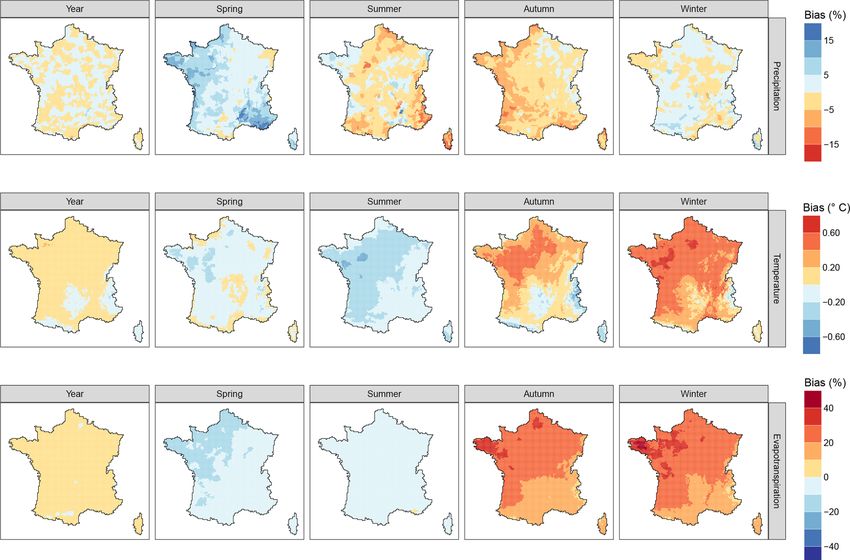
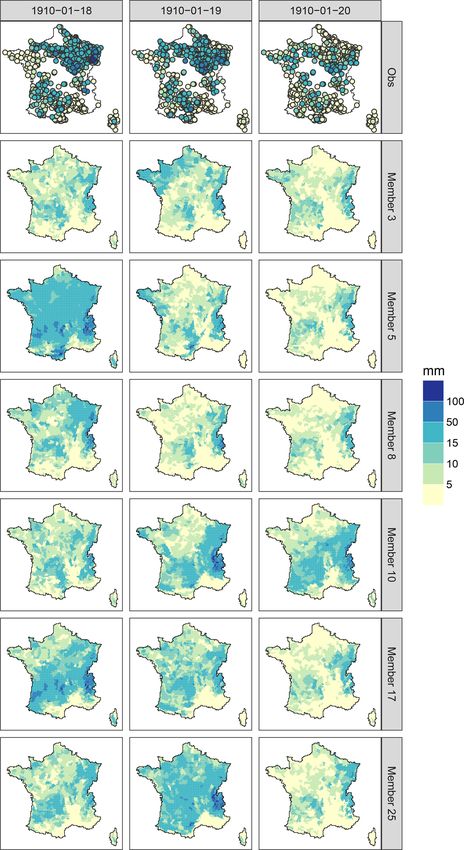
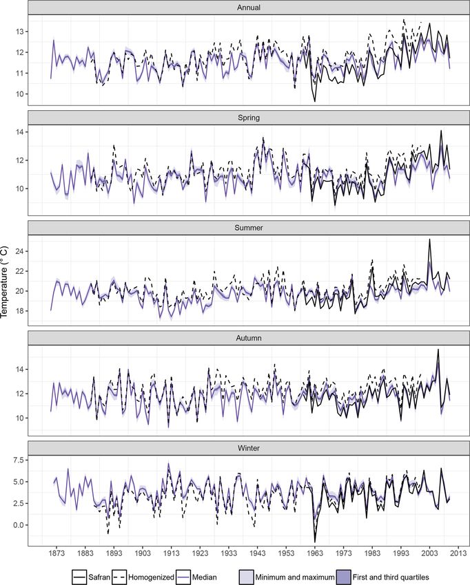
246                                                                                           L. Caillouet et al.: SCOPE Climate

Figure 2. Synthetic diagram showing the sequence of steps for the SCOPE method and its use for SCOPE Climate reconstructions. Repro-
duced from Caillouet et al. (2016).

servations: Picardie (north), the main part of the Loire basin      3.1.2   Temporal features: time series at Lyon–Bron
(centre), Jura mountain range (east), most of the Alps, and                 Airport
Provence (south-east).
   Concurrent SCOPE Climate precipitation reconstructions           The evaluation of SCOPE Climate against independent data
are presented on rows 2–7 of Fig. 3 with six randomly se-           is possible using homogenized series provided by Météo-
lected members. Some members provide high amounts of                France (Moisselin et al., 2002; Moisselin and Schneider,
precipitation for almost the whole of France (on 18 January         2002). These series were computed at a monthly time step
for member 5 and on 19 January for member 25) with an               using a statistical procedure detecting breaks and outliers in
emphasis on mountain ranges (Vosges, Jura, and the French           long time series of observations with sufficient quality. The
Alps). Some members provide high precipitation amounts on           323 monthly precipitation series and 65 monthly time series
a diagonal from the north-east to the south-west (on 19 and         of minimum and maximum temperature spanning the whole
20 January for member 10 and on the 18 January for member           of the 20th century were retained for the evaluation. Monthly
17). Others provide high precipitation for particular zones in      mean temperature time series were obtained by averaging
France (Brittany for member 3 on 19 January, east for mem-          minimum and maximum temperatures as done by Moisselin
ber 8 on the 8 January). Four members out of the six ran-           and Schneider (2002). The closest 8 km grid point to the ob-
domly selected members provide more than 100 mm of pre-             servation station is selected for the comparison. It has to be
cipitation for the French Alps and Jura on a particular day         noted that comparisons between gridded products like Safran
(members 5, 10, 17, and 25), a zone without available pre-          or SCOPE Climate and station data should be taken with cau-
cipitation observations but where important floods have been        tion as corresponding variables may have different proper-
recorded (Boudou et al., 2016).                                     ties, e.g. due to spatial representativity and altitude.
   Figure 4 provides the maps of surface temperature for the           The Lyon–Bron Airport station holds very long time se-
18 to 20 January 1910 from available observations (top) and         ries (since 1881 for precipitation and 1885 for temperature)
the same six selected members of SCOPE Climate. Spa-                already used in climate variability studies (see e.g. Thib-
tial patterns of reconstructed temperature are in good agree-       ert et al., 2013). Here the annual and seasonal evolution of
ment with each other and with observations. Values are              precipitation are compared (Fig. 5), as well as temperature
largely positive over the Seine catchment, in agreement with        (Fig. 6) from (1) the homogenized series, (2) Safran data, and
snowmelt records. This example demonstrates the ability of          (3) the range of reconstructed series from SCOPE Climate.
SCOPE Climate to fill in the spatial gaps of missing data and          Precipitation reconstructions from Fig. 5 show a very sat-
to provide a spatially coherent reconstruction of temperature.      isfactorily reconstructed interannual variability on the annual

Earth Syst. Sci. Data, 11, 241–260, 2019                                              www.earth-syst-sci-data.net/11/241/2019/
L. Caillouet et al.: SCOPE Climate                                                                                                247

Figure 3. 18 to 20 January 1910 precipitation. Top: observations currently available from the Météo-France database. Rows 2–7: six ran-
domly selected members of SCOPE Climate.

www.earth-syst-sci-data.net/11/241/2019/                                                Earth Syst. Sci. Data, 11, 241–260, 2019
248 L. Caillouet et al.: SCOPE Climate
1910−01−18 1910−01−19 1910−01−20
● ● ●
●● ●
● ● ●● ●
● ● ●● ●
● ●
● ● ●
● ●
● ● ● ●
● ●
● ● ● ●
● ●
●
●●
● ●●
● ●●
●
● ● ●●●●●● ● ● ●●●●●● ● ● ●●●●●●
● ● ● ● ● ● ● ● ●
Obs
● ● ● ● ● ● ● ● ●
● ●● ● ●● ● ●●
● ● ●● ●● ● ● ●● ●● ● ● ●● ●●
●
● ●
● ●
●
●●●● ●● ● ●●●● ●● ● ●●●● ●● ●
● ● ●
● ●● ● ● ●● ● ● ●● ●
● ●●●●●
●
●
● ● ●●●●●
●
●
● ● ●●●●●
●
●
●
● ● ● ● ● ● ● ● ●
● ● ●● ● ● ● ●● ● ● ● ●● ●
●●
●● ●●
●● ●●
●●
●
●●● ●
●●● ●
●●●
Member 3
Member 5
°C
16
Member 8
12
8
4
0
Member 10
Member 17
Member 25
Figure 4. As for Fig. 3, but for mean temperature.
Earth Syst. Sci. Data, 11, 241–260, 2019 www.earth-syst-sci-data.net/11/241/2019/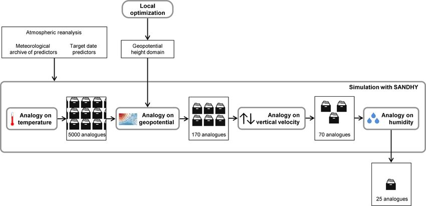
L. Caillouet et al.: SCOPE Climate                                                                                                     249

Figure 5. Lyon–Bron precipitation homogenized time series, corresponding Safran data, and reconstructed series from SCOPE Climate on
the annual and seasonal timescales over the 1871–2012 time period. Light and dark purple areas define the range and the interquartile range,
respectively, of values from SCOPE Climate members. Note the different scales for the y axes.

and seasonal timescales. Except for some specific years, ob-            well captured by SCOPE Climate. The few years before 1897
servations (from both homogenized series and Safran) stay               show a lower reconstruction skill. SCOPE Climate shows
inside the range of the 25 reconstructions. On the annual               a high annual precipitation in 1872, for which no data are
timescale, exceptional years – such as the 1921 dry year                available. Nevertheless, Gautier et al. (2004) described one
(Duband et al., 2004) or the 1960 wet year (Pardé, 1961) – are          of the biggest floods in the Loire basin, in October 1872, and

www.earth-syst-sci-data.net/11/241/2019/                                                    Earth Syst. Sci. Data, 11, 241–260, 2019
250                                                                                    L. Caillouet et al.: SCOPE Climate

Figure 6. As for Fig. 5, but for temperature.

heavy precipitation in Roanne and Macon, two towns close to      Temperature reconstructions from Fig. 6 are compared
Lyon. SCOPE Climate has difficulty simulating the extreme     between the different datasets on annual and seasonal
wet spring and dry summer of 1983 (Blanchet, 1984). Nev-      timescales. The interannual variability is quite satisfactorily
ertheless, other extreme events like the wet winter of 1936   simulated, but the uncertainty in the reconstructions seems
(Pardé, 1937) are well simulated.                             underestimated, with observations being too often out of the
                                                              range of SCOPE Climate members. Summer temperatures

Earth Syst. Sci. Data, 11, 241–260, 2019                                       www.earth-syst-sci-data.net/11/241/2019/
L. Caillouet et al.: SCOPE Climate 251
are generally underestimated, whereas winter temperatures remains outside of the Safran archive period used to cre-
are generally overestimated, leading to a systematic under- ate SCOPE Climate (1958–2008) and is among the hottest
or overestimation of temperature in hot or cold years. How- years since 19002 . Precipitation, temperature, and evapo-
ever, the recent trend in spring and summer temperature is transpiration time series from both Safran and SCOPE Cli-
captured – although underestimated – by the reconstruction mate are presented in Fig. 8 for the Finistère grid cell (see
method. Fig. 7). Safran precipitation is included most of the time
Some hot seasons are well captured, such as the 1942– in the range of the 25 reconstructions, except for extremely
1948 period for spring, and especially the hot spring of 1945 wet days above 20 mm. There are only a few days on which
(Martin, 1946) or the more recent hot summer of 1976 (Bro- both Safran and all 25 members reconstruct zero precipita-
chet, 1977). The cold autumn of 1912 is also well cap- tion. Nevertheless, the sequence of alternating dry and wet
tured by SCOPE Climate (Puiseux, 1913, p. 63). Tempera- periods is well respected in SCOPE Climate. Member 1 pro-
ture for other events like the extremely cold winter 1962– vides a good reconstruction of Safran precipitation with a
1963 (Geneslay, 1964) or the recent hot summer of 2003 slight overestimation for moderate episodes and an underes-
(Trigo et al., 2005) are, however, over- or underestimated timation for strong episodes. Safran temperature is almost
(about +2 ◦ C for 1963 and −2.3 ◦ C for 2003 in comparison always included in the – sometimes very thin – range of
to Safran), but still captured. SCOPE Climate temperatures, showing the small bias of the
SCOPE method. The overall Safran variability is well recon-
3.2 Performance of SCOPE Climate against reference
structed by Member 1 of SCOPE Climate. The good results
datasets
obtained for precipitation and temperature do not apply to
evapotranspiration. Indeed, even if Safran evapotranspiration
The performance of SCOPE Climate is assessed using Safran is included in the extremely large range of SCOPE Climate
as reference dataset. First, direct comparisons to Safran are reconstructions, the day-to-day variability reconstructed by
made through the use of interannual regimes and visualiza- Member 1 is far too high in comparison to Safran, especially
tion of time series at a daily time step in a specific year. Then, in winter. Moreover, the sign of these day-to-day variations
different skill scores are used to complete the validation of (increase or decrease) is sometimes not the same for Safran
SCOPE Climate. and Member 1 of SCOPE Climate. In spite of a good re-
construction of precipitation and temperature, evapotranspi-
3.2.1 Performance against the Safran reanalysis
ration results lack autocorrelation. Caution is therefore re-
quired if SCOPE Climate is used for studying specific events
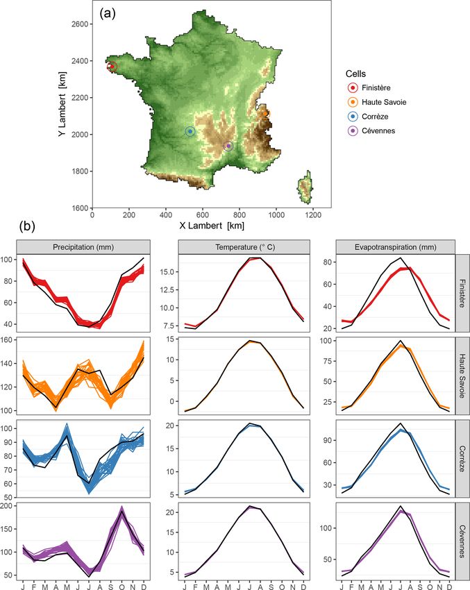
The interannual regimes from Safran and SCOPE Climate for which evapotranspiration plays an important role, such as
precipitation, temperature, and reference evapotranspiration the 2003 drought (Teuling et al., 2013).
are compared to each other on four different case study cells, Figure 9 shows the median of annual and seasonal pre-
belonging to four regions with very different climatic influ- cipitation, temperature and reference evapotranspiration bias
ences (Fig. 7). Precipitation regimes are well reconstructed between Safran and SCOPE Climate over the 1959–2007 pe-
by SCOPE Climate. Spring precipitation is slightly overes- riod (complete years in the archive period). The median of
timated, whereas autumnal precipitation can be slightly un- annual precipitation bias between Safran and SCOPE Cli-
derestimated (for Finistère and Corrèze). These results show mate shows an absolute value under 5 % for the whole of
that the SCOPE method is able to reproduce strong seasonal France, except for a specific area in the Cévennes region (top
cycles (asymmetry between spring and autumn) as well as row of Fig. 9). In summer, autumn, and winter, the bias is
continental regimes. For temperature, the Safran regime is generally under 5 % in absolute value and up to ±15 % for
always inside the thin range of SCOPE Climate regimes in specific areas. Spring precipitation is overestimated for the
spring and autumn for all cells. Temperatures are slightly Atlantic coast and the Mediterranean region. As spring is the
overestimated in winter and underestimated in summer. The only season showing an overestimation of precipitation after
regimes of reference evapotranspiration show differences be- the second step of the SCOPE method (see Sect. 2.2.2), re-
tween Safran and SCOPE Climate. For all cells, evapotran- moving dry days for this season as done in Sect. 2.2.3 will
spiration is underestimated in spring and summer and over- exacerbate the precipitation overestimation. This could be
estimated in autumn and winter. Moreover, for the Finistère, managed by adapting the number of dry days to be removed
SCOPE Climate maximum evapotranspiration is not seen in depending on the season, as it is done for the zones. Never-
July, as for Safran, but in August, leading to a shifted sea- theless, for the sake of parsimony and because the bias cor-
sonal cycle. This shows the importance of variables other rection is already adapted to each zone, the choice was made
than temperature in the computation of reference evapotran- to have the same parameters for all seasons. The median of
spiration and a lack of information on these variables in
SCOPE predictors. 2 http://www.meteofrance.fr/climat-passe-et-futur/
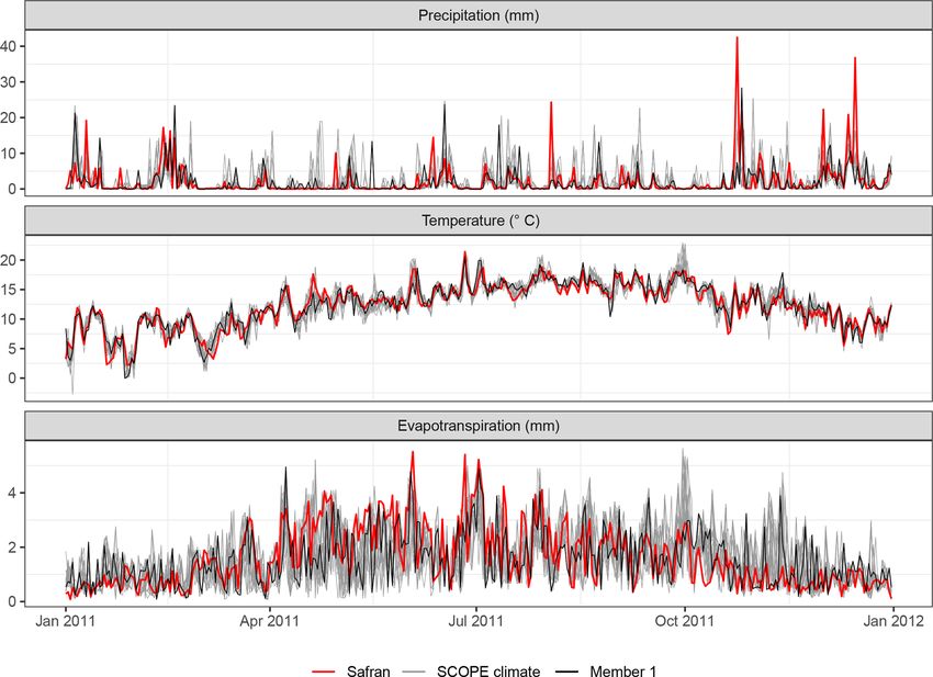
The year 2011 has been chosen as an example to show bilans-climatiques/autres-annees/bilan-de-lannee-2011 (last
SCOPE Climate and Safran at a daily time step. This year access: 20 February 2018).
www.earth-syst-sci-data.net/11/241/2019/ Earth Syst. Sci. Data, 11, 241–260, 2019252 L. Caillouet et al.: SCOPE Climate Figure 7. (a) Topographical map of France with location of the 4 case study cells: Finistère in Brittany, Haute-Savoie in the French Alps, Corrèze in the south-west, and Cévennes in the Massif Central mountain range. Brown corresponds to altitudes above 650 m (up to 2933 m). Green corresponds to altitudes under 500 m. (b) Precipitation, temperature, and reference evapotranspiration interannual regimes between 1959 and 2007 from Safran (black) and SCOPE Climate (colours), through the 25 individual members, for the case study cells. Earth Syst. Sci. Data, 11, 241–260, 2019 www.earth-syst-sci-data.net/11/241/2019/
L. Caillouet et al.: SCOPE Climate                                                                                                  253

Figure 8. Precipitation, temperature, and reference evapotranspiration reconstructed series from SCOPE Climate compared to Safran in
2011 at a daily time step for the Finistère grid cell (see Fig. 7). Light grey time series correspond to the 25 members of SCOPE Climate,
Member 1 is plotted in black for exemplifying autocorrelation in individual member time series.

annual and seasonal temperature bias is low (middle row of             period shows values above 0.6 except for the south-east of
Fig. 9). It is limited to ±0.20 ◦ C on the annual scale and gen-       France (Fig. 10). Correlations are similar for the spring sea-
erally stays under ±0.60 ◦ C on the seasonal scale. The max-           son, but are lower for summer. This can be explained by
imum bias is reached for a small region in the north-west of           the numerous local storms occurring in summer, which are
France and around Paris with an overestimation of +0.63 ◦ C            hardly predictable by the SCOPE method. Precipitation cor-
in winter. The median evapotranspiration bias is kept under            relations are generally above 0.8 in autumn and winter. The
±10 % on the annual timescale, and largely under ±20 % in              median of correlations for temperature shows values gener-
spring and summer. This bias is higher in autumn and es-               ally above 0.8–0.9 for the annual and seasonal time steps,
pecially in winter, with an overestimation of evapotranspi-            with only a few zones in autumn showing lower values.
ration between 30 % and 40 % for the north-east of France              For reference evapotranspiration, the median correlations are
(up to 50 % for Brittany). The SCOPE method has not been               generally above 0.6 for all time steps, except for winter when
adapted for reference evapotranspiration specifically, and the         a large part of France shows low correlations. This last result
results obtained for this variable should therefore be taken           is consistent with results from Fig. 8.
with care. Evapotranspiration biases are due to a larger se-              The continuous ranked probability score (CRPS, Brown,
lection of analogue days in other seasons than the target day          1974; Matheson and Winkler, 1976) is used to compute a
season. This feature, strongly present in SANDHY outputs,              probabilistic evaluation of SCOPE Climate at daily, monthly,
has been reduced with the addition of the stepwise subse-              and annual time steps. This score is equivalent to the mean
lection (see Sect. 2.2.2). Nevertheless, this is not enough to         absolute error in a deterministic context. After normalization
remove the biases in reference evapotranspiration.                     by a climatological reference, the continuous ranked prob-
   The median of annual correlations between Safran precipi-           ability skill score (CRPSS; see Sect. 3.4 in Caillouet et al.,
tation and SCOPE Climate precipitation over the 1959–2007              2016, for more details) allows for a comparison of zones with

www.earth-syst-sci-data.net/11/241/2019/                                                  Earth Syst. Sci. Data, 11, 241–260, 2019
254                                                                                           L. Caillouet et al.: SCOPE Climate

Figure 9. Median of annual and seasonal precipitation (top row), temperature (middle row), and evapotranspiration (bottom row) bias
between Safran and SCOPE Climate for the 1959–2007 period. Red corresponds to an overestimation of the reconstructed temperature and
reference evapotranspiration as well as an underestimation of the reconstructed precipitation.

different climates. Here, the climatology is calculated using       daily and monthly time steps: the highest scores are found for
data from Safran over the archive period (1958–2008), tak-          the south-east of France, and particularly for the French Alps
ing seasonality into account. The CRPSS is shown in Fig. 11         and the western part of Massif Central. The lowest scores
for all variables of SCOPE Climate and all time steps. Posi-        are found for the north-west of France, and the major part of
tive CRPSS values denote an improved skill with respect to          France shows negative values at the monthly time step. This
the climatology, and 1 reflects a perfect reconstruction. For       negative skill is partly explained by the shifted seasonal cycle
precipitation, the spatial distribution of the CRPSS is similar     (see Fig. 7) in addition to the seasonal bias (see Fig. 9). As for
for the three time steps. The lowest performances are found         temperature, the spatial distribution of CRPSS at the annual
for the Mediterranean coast, the east of France, Corsica, and       time step shows relatively high spatial discontinuities. Most
the eastern part of Massif Central. The highest CRPSS val-          of France shows positive annual values, except for Corsica,
ues are found for the Atlantic coast, the French Alps, the          where strong negative values are found.
Cévennes area, and the western parts of the Massif Central,
Jura, and Vosges mountain ranges. For temperature, the high-        3.3   Performance against homogenized times series
est scores for the daily and monthly time steps are obtained
for mountainous areas, while the lowest ones are obtained for       The evolution of the spatially averaged root mean square
the north-west (only for the monthly time step), south-east,        error (RMSE) for both Safran and SCOPE Climate is pre-
and Corsica. A much smoother spatial distribution is found at       sented in Fig. 12 using the homogenized series as a reference.
the daily and monthly time steps compared to the annual time        Monthly RMSEs are first calculated using the 323 precipita-
step. At the annual time step, the highest scores are obtained      tion time series and the 65 temperature time series. This leads
for the north-west of France, and some specific cells in the        to one value of RMSE per month for Safran and 25 values
south-east have a negative CRPSS. For reference evapotran-          of RMSE per month for SCOPE Climate. These RMSEs are
spiration, the spatial distribution of CRPSS is similar at the      then averaged yearly for each SCOPE Climate member. The
                                                                    RMSE in mm yr−1 is then divided by the number of days in

Earth Syst. Sci. Data, 11, 241–260, 2019                                              www.earth-syst-sci-data.net/11/241/2019/
L. Caillouet et al.: SCOPE Climate 255
Figure 10. Median of annual and seasonal precipitation (top row), temperature (middle row), and reference evapotranspiration (bottom row)
correlation between Safran and SCOPE Climate for the 1959–2007 period.
each year to get an RMSE in mm day−1 . Coloured intervals to create the SCOPE Hydro dataset that provides ensemble
then show the range between minimum and maximum an- daily streamflow time series for more than 600 near-natural
nual values of the 25 members. For precipitation, RMSEs are catchments in France over the 1871–2012 period (Caillouet
relatively constant over time, with an average value around et al., 2017). It has also been used to study spatio-temporal
1.3 mm day−1 . They are, however, slightly higher before the extreme low-flow events in France since 1871 by Caillouet
1940s. It is important to note that Safran errors, which were et al. (2017).
documented by Vidal et al. (2010), account for nearly half The SCOPE Climate dataset is available under the
(around 0.6 mm day−1 ) of the reconstruction errors. For tem- Attribution-NonCommercial 4.0 International (CC BY-NC
perature, SCOPE Climate RMSEs are around 1 ◦ C over the 4.0): One may copy and redistribute the material in any
entire period. It even reaches down to 0.9 ◦ C over 1959–2000 medium or format, remix, transform and build upon the ma-
when Safran errors are around 0.8 ◦ C. terial with the following terms: (1) Attribution – one must
give appropriate credit, provide a link to the license, and in-
dicate whether changes were made. One may do so in any
4 Data availability
reasonable manner, but not in any way that suggests the li-
censor endorses you or your use. (2) NonCommercial – one
SCOPE Climate is a 142-year high-resolution ensemble
may not use the material for commercial purposes.
gridded daily meteorological reconstruction of precipitation,
SCOPE Climate is available through the Zenodo repos-
temperature and reference evapotranspiration over France.
itory (http://zenodo.org, last access: 14 February 2019), as
This dataset is the result of the statistical downscaling of
three different datasets, with one for each variable (pre-
20CR by the SCOPE method. Results are available for 25
cipitation, temperature, and reference evapotranspiration).
members at a daily time step and over a 8 km grid. This
Each dataset stores 25 NetCDF files corresponding to the 25
dataset is spatially coherent over France and has a high inter-
SCOPE Climate members. Please note that when using mul-
variable coherence, thus enabling studies requiring spatial
tiple variables simultaneously, e.g. precipitation and temper-
and multi-variable meteorological variables, such as hydro-
ature, one may use precipitation from member 1 with tem-
logical studies. SCOPE Climate has been used as forcings
www.earth-syst-sci-data.net/11/241/2019/ Earth Syst. Sci. Data, 11, 241–260, 2019256 L. Caillouet et al.: SCOPE Climate Figure 11. Daily, monthly, and annual CRPSS between SCOPE Climate and Safran for precipitation, temperature, and reference evapotran- spiration over the 1959–2007 period. Note the different scales across the maps. Figure 12. Temporal evolution of the precipitation and temperature RMSE for both Safran and SCOPE Climate, with the homogenized series as a reference. Values are initially computed on the monthly timescale. See text for details. Earth Syst. Sci. Data, 11, 241–260, 2019 www.earth-syst-sci-data.net/11/241/2019/
L. Caillouet et al.: SCOPE Climate                                                                                               257

perature from member 1 (and member 2 with member 2), as              Convective precipitation events usually stem from very
SCOPE Climate provides consistent gridded values across           local processes and are therefore hardly detectable from
variables for any single member. SCOPE Climate can be             only large-scale information. This is why downscaling meth-
downloaded as NetCDF files for precipitation (Caillouet et        ods have some difficulty in reconstructing such events, and
al., 2018a), temperature (Caillouet et al., 2018b), and refer-    SANDHY (and thus SCOPE) is no exception. For this rea-
ence evapotranspiration (Caillouet et al., 2018c).                son, SCOPE Climate should not be used to study specifically
                                                                  convective events.
                                                                     Finally, as the downscaling method is based on the ana-
5   Conclusions                                                   logue principle, it is not possible to reconstruct higher (for
                                                                  precipitation, temperature and reference evapotranspiration)
The use of SCOPE Climate is conditional on the large-scale        or lower (for temperature) values than the ones available in
information provided by the 20CR atmospheric reanalysis,          the archive dataset. Nevertheless, values averaged over sev-
and using an alternative extended reanalysis like ERA-20C         eral days or over several climatically homogeneous zones
may lead to different outputs (see Dayon et al., 2015; Horton     may exceed these limits. The performance of SCOPE Cli-
and Brönnimann, 2018). SCOPE Climate takes into account           mate in reconstructing convective precipitation events has
the uncertainty related to the SCOPE method, but not the un-      not been assessed and may be lower than for stratiform events
certainty related to 20CR, as only the ensemble mean has          as relevant information may not be included in large-scale
been considered. As discussed by Caillouet et al. (2016), the     predictors of the SCOPE method.
different members of 20CR show an increased spread before
the 1930s–1940s, because of too few data assimilated during
this period. SCOPE Climate might thus show a lower quality        Author contributions. LC developed the dataset and prepared the
before this period. Similarly, using another statistical down-    manuscript. JPV, ES, and BG contributed to the development of
scaling method from either 20CR or ERA20C may lead to             the dataset. JMS supplied the Safran reanalysis. All co-authors con-
different outputs (see e.g. Horton and Brönnimann, 2018).         tributed to the manuscript.
   Results for reference evapotranspiration showed weak per-
formances at daily and monthly time steps. This issue could
                                                                  Competing interests. The authors declare that they have no con-
be fixed by having some kind of calendar selection in the
                                                                  flict of interest.
downscaling process. Ben Daoud et al. (2011), however,
showed that the performance in estimating precipitation is
lower when replacing the first analogy level in SANDHY            Acknowledgements. Support for the Twentieth Century Reanal-
with a calendar preselection. Caillouet et al. (2016) addition-   ysis Project dataset is provided by the U.S. Department of Energy,
ally showed that having a stepwise subselection of SANDHY         Office of Science Innovative and Novel Computational Impact on
outputs led to higher rank correlations and lower mean er-        Theory and Experiment (DOE INCITE) programme, and Office of
rors between observed and reconstructed temperatures than a       Biological and Environmental Research (BER), and by the National
calendar subselection. Moreover, setting fixed seasons would      Oceanic and Atmospheric Administration Climate Program Office.
not be necessarily suitable for our case – a long-term histor-    The authors would like to thank Météo-France for providing
ical reconstruction – as there could be season shifts. Thus,      access to the Safran database. Analyses were performed in R (R
it is not recommended to use SCOPE Climate for studies            Core Team, 2016), with packages dplyr (Wickham and Francois,
specifically on evapotranspiration. Nevertheless, it is possi-    2015), ggplot2 (Wickham, 2009), RColorBrewer (Neuwirth, 2014),
                                                                  reshape2 (Wickham, 2007), sp (Pebesma and Bivand, 2005; Bivand
ble to use this variable in hydrological modelling for regions
                                                                  et al., 2013), grid (R Core Team, 2016), gridExtra (Auguie, 2016),
and/or temporal periods where/when this variable is not the       and scales (Wickham, 2016). Laurie Caillouet’s PhD thesis was
main driver of streamflow. Caillouet et al. (2017) showed that    funded by Irstea and CNR.
streamflow reconstructions driven by SCOPE Climate have a
high skill for most of the 662 near-natural catchments con-       Edited by: David Carlson
sidered across France.                                            Reviewed by: two anonymous referees
   Time series were constructed in SCOPE Climate by inde-
pendently combining analogue dates from one day to another
and the only temporal coherence is ensured by that of the
                                                                  References
large-scale predictors. The Schaake Shuffle allows, in a fore-
casting context, for a temporal coherence to be retrieved over
                                                                  Allen, R. G., Pereira, L. S., Raes, D., and Smith, M.: Crop Evap-
the forecast horizon, on top of the spatial and inter-variable      otranspiration – Guidelines for computing crop water require-
coherence. Such a desirable property is, however, hampered          ments, FAO Irrigation and Drainage Paper 56, FAO, Rome, 1998.
here by the length over which temporal coherence is required      Auguie, B.: gridExtra: Miscellaneous Functions for “Grid” Graph-
(142 years), which is larger than the archive period (50 years)     ics, available at: https://CRAN.R-project.org/package=gridExtra
from which this empirical coherence can be extracted.               (last access: 14 February 2019), R package version 2.2.1, 2016.

www.earth-syst-sci-data.net/11/241/2019/                                               Earth Syst. Sci. Data, 11, 241–260, 2019
258 L. Caillouet et al.: SCOPE Climate Ben Daoud, A., Sauquet, E., Lang, M., Bontron, G., and T. F., Trigo, R. M., Wang, X. L., Woodruff, S. D., and Worley, Obled, C.: Precipitation forecasting through an analog sorting S. J.: International Surface Pressure Databank (ISPDv2), 2010. technique: a comparative study, Adv. Geosci., 29, 103–107, Compo, G. P., Whitaker, J. S., Sardeshmukh, P. D., Matsui, N., Al- https://doi.org/10.5194/adgeo-29-103-2011, 2011. lan, R. J., Yin, X., Gleason, B. E., Vose, R. S., Rutledge, G., Ben Daoud, A., Sauquet, E., Bontron, G., Obled, C., and Bessemoulin, P., Brönnimann, S., Brunet, M., Crouthamel, R. I., Lang, M.: Daily quantitative precipitation forecasts based Grant, A. N., Groisman, P. Y., Jones, P. D., Kruk, M. C., Kruger, on the analogue method: Improvements and application to A. C., Marshall, G. J., Maugeri, M., Mok, H. Y., Nordli, Ø., Ross, a French large river basin, Atmos. Res., 169, 147–159, T. F., Trigo, R. M., Wang, X. L., Woodruff, S. D., and Worley, https://doi.org/10.1016/j.atmosres.2015.09.015, 2016. S. J.: The Twentieth Century Reanalysis Project, Q. J. Roy. Me- Bivand, R. S., Pebesma, E., and Gomez-Rubio, V.: Applied spa- teor. Soc., 137, 1–28, https://doi.org/10.1002/qj.776, 2011. tial data analysis with R, Second edition, Springer, NY, available Dayon, G., Boé, J., and Martin, E.: Transferability in the fu- at: http://www.asdar-book.org/ (last access: 14 February 2019), ture climate of a statistical downscaling method for pre- 2013. cipitation in France, J. Geophys. Res., 120, 1023–1043, Blanchet, G.: Le temps dans la région Rhóne- https://doi.org/10.1002/2014JD022236, 2015. Alpes en 1983, Géocarrefour, 59, 347–365, Delserieys, M. and Blanchard, R.: District Seine-Normandie, in: https://doi.org/10.3406/geoca.1984.4041, 1984. Les inondations remarquables en France, edited by: Lang, M. Bonnet, R., Boé, J., Dayon, G., and Martin, E.: Twentieth-century and Cœur, D., chap. 6, 381–456, Quæ, Versailles, France, 2014. hydrometeorological reconstructions to study the multidecadal Duband, D., Schoeneich, P., and Stanescu, V. A.: The example variations of the water cycle over France, Water Resour. Res., of 1921 drought in Europe (Italy, France, Romania, Switzer- 53, 8366–8382, https://doi.org/10.1002/2017WR020596, 2017. land...): climatology and hydrology, Houille Blanche, 18–29, Boudou, M., Danière, B., and Lang, M.: Assessing changes in https://doi.org/10.1051/lhb:200405001, 2004. urban flood vulnerability through mapping land use from his- Gautier, J.-N., Mergenthaler, S., and Camp’Huis, N.-G.: torical information, Hydrol. Earth Syst. Sci., 20, 161–173, La crue d’octobre 1872 en France (Loire), en Italie https://doi.org/10.5194/hess-20-161-2016, 2016. (Po) et en Espagne (Ebre), Houille Blanche, 56–63, Brochet, P.: La sécheresse 1976 en France: aspects clima- https://doi.org/10.1051/lhb:200405007, 2004. tologiques et conséquences, Hydrol. Sci. B., 22, 393–411, Geneslay, E.: L’hiver 1962–1963, L’Astronomie, 78, 110–111, https://doi.org/10.1080/02626667709491733, 1977. available at: http://adsabs.harvard.edu/full/1964LAstr..78..110G Brown, T. A.: Admissible scoring systems for continuous distri- (last access: 14 February 2019), 1964. butions, Tech. rep., The Rand Corporation, Santa Monica, CA, Horton, P. and Brönnimann, S.: Impact of global atmospheric re- 1974. analyses on statistical precipitation downscaling, Clim. Dynam., Caillouet, L., Vidal, J.-P., Sauquet, E., and Graff, B.: Probabilis- https://doi.org/10.1007/s00382-018-4442-6, 2018. tic precipitation and temperature downscaling of the Twenti- Jourdain, S., Roucaute, E., Dandin, P., Javelle, J.-P., Donet, I., Mé- eth Century Reanalysis over France, Clim. Past, 12, 635–662, nassère, S., and Cénac, N.: Le sauvetage de données clima- https://doi.org/10.5194/cp-12-635-2016, 2016. tologiques anciennes à Météo-France: De la conservation des Caillouet, L., Vidal, J.-P., Sauquet, E., Devers, A., and Graff, B.: documents à la mise à disposition des données, La Météorolo- Ensemble reconstruction of spatio-temporal extreme low-flow gie, 47–55, https://doi.org/10.4267/2042/56598, 2015. events in France since 1871, Hydrol. Earth Syst. Sc., 21, 2923– Keller, V. D. J., Tanguy, M., Prosdocimi, I., Terry, J. A., Hitt, O., 2951, https://doi.org/10.5194/hess-21-2923-2017, 2017. Cole, S. J., Fry, M., Morris, D. G., and Dixon, H.: CEH-GEAR: Caillouet, L., Vidal, J.-P., Sauquet, E., Graff, B., and Soubeyroux, 1 km resolution daily and monthly areal rainfall estimates for the J.-M.: SCOPE Climate: precipitation (Version v1.0.0), [Data set], UK for hydrological and other applications, Earth Syst. Sci. Data, Zenodo, https://doi.org/10.5281/zenodo.1299760, 2018a. 7, 143–155, https://doi.org/10.5194/essd-7-143-2015, 2015. Caillouet, L., Vidal, J.-P., Sauquet, E., Graff, B., and Soubeyroux, Kuentz, A., Mathevet, T., Gailhard, J., and Hingray, B.: Build- J.-M.: SCOPE Climate: temperature (Version v1.0.0), [Data set], ing long-term and high spatio-temporal resolution precipitation Zenodo, https://doi.org/10.5281/zenodo.1299712, 2018b. and air temperature reanalyses by mixing local observations and Caillouet, L., Vidal, J.-P., Sauquet, E., Graff, B., and Soubey- global atmospheric reanalyses: the ANATEM method, Hydrol. roux, J.-M.: SCOPE Climate: Penman-Monteith reference Earth Syst. Sc., 19, 2717–2736, https://doi.org/10.5194/hess-19- evapotranspiration (Version v1.0.0), [Data set], Zenodo, 2717-2015, 2015. https://doi.org/10.5281/zenodo.1251843, 2018c. Lang, M., Cœur, D., Bard, A., Bacq, B., Becker, T., Bignon, E., Clark, M., Gangopadhyay, S., Hay, L., Rajagopalan, Blanchard, R., Bruckmann, L., Delserieys, M., Edelblutte, C., B., and Wilby, R.: The Schaake Shuffle: A Method and Merle, C.: Les inondations remarquables en France : pre- for reconstructing space-Time variability in fore- miers éléments issus de l’enquête EPRI 2011, Houille Blanche, casted precipitation and temperature fields, J. Hy- 37–47, https://doi.org/10.1051/lhb/2013041, 2013. drometeorol., 5, 243–262, https://doi.org/10.1175/1525- Lorenz, E. N.: Atmospheric predictability as re- 7541(2004)0052.0.CO;2, 2004. vealed by naturally occurring analogues, J. At- Compo, G. P., Whitaker, J. S., Sardeshmukh, P. D., Matsui, N., Al- mos. Sci., 26, 636–646, https://doi.org/10.1175/1520- lan, R. J., Yin, X., Gleason, B. E., Vose, R. S., Rutledge, G., 0469(1969)262.0.CO;2, 1969. Bessemoulin, P., Bronnimann, S., Brunet, M., Crouthamel, R. I., Marti, R. and Lepelletier, T.: L’hydrologie de la crue de 1910 et Grant, A. N., Groisman, P. Y., Jones, P. D., Kruk, M. C., Kruger, autres grandes crues du bassin de la Seine, Houille Blanche, 33– A. C., Marshall, G. J., Maugeri, M., Mok, H. Y., Nordli, O., Ross, 39, https://doi.org/10.1051/lhb/1997074, 1997. Earth Syst. Sci. Data, 11, 241–260, 2019 www.earth-syst-sci-data.net/11/241/2019/
You can also read