The role of storm scale, position and movement in controlling urban flood response - HESS
←
→
Page content transcription
If your browser does not render page correctly, please read the page content below
Hydrol. Earth Syst. Sci., 22, 417–436, 2018
https://doi.org/10.5194/hess-22-417-2018
© Author(s) 2018. This work is distributed under
the Creative Commons Attribution 3.0 License.

The role of storm scale, position and movement in
controlling urban flood response
Marie-claire ten Veldhuis1,2 , Zhengzheng Zhou2,3,4 , Long Yang2 , Shuguang Liu4 , and James Smith2
1 DelftUniversity of Technology, Watermanagement Department, Delft, 2628CN, the Netherlands
2 PrincetonUniversity, Hydrometeorology Group, Princeton, NJ 08544, USA
3 Tongji University, School of Ocean and Earth Science, Shanghai, 200092, China
4 UNEP-Tongji Institute of Environment for Sustainable Development Shanghai, Shanghai, 20002 China

Correspondence: Marie-claire ten Veldhuis (j.a.e.tenveldhuis@tudelft.nl) and Zhengzheng Zhou
(zhouzhengzhengzzz@126.com)

Received: 3 April 2017 – Discussion started: 15 May 2017
Revised: 14 November 2017 – Accepted: 14 November 2017 – Published: 18 January 2018

Abstract. The impact of spatial and temporal variability of       cover within the basins had little effect on flow peaks. These
rainfall on hydrological response remains poorly understood,      findings show the importance of observation-based analysis
in particular in urban catchments due to their strong vari-       in validating and improving our understanding of interac-
ability in land use, a high degree of imperviousness and the      tions between the spatial distribution of rainfall and catch-
presence of stormwater infrastructure. In this study, we an-      ment variability.
alyze the effect of storm scale, position and movement in
relation to basin scale and flow-path network structure on
urban hydrological response. A catalog of 279 peak events
was extracted from a high-quality observational dataset cov-      1   Introduction
ering 15 years of flow observations and radar rainfall data for
five (semi)urbanized basins ranging from 7.0 to 111.1 km2         The interactions between spatial and temporal variability of
in size. Results showed that the largest peak flows in the        rainfall and hydrological response characteristics have been
event catalog were associated with storm core scales ex-          the topic of numerous empirical and modeling studies in re-
ceeding basin scale, for all except the largest basin. Spatial    cent decades (Anquetin et al., 2010; Lobligeois et al., 2014;
scale of flood-producing storm events in the smaller basins       Morin et al., 2006; Segond et al., 2007; Syed et al., 2003;
fell into two groups: storms of large spatial scales exceed-      Tetzlaff and Uhlenbrook, 2005; Volpi et al., 2012; Yakir and
ing basin size or small, concentrated events, with storm core     Morin, 2011). They have shown that interactions depend on
much smaller than basin size. For the majority of events, spa-    the complex interplay between rainfall variability and catch-
tial rainfall variability was strongly smoothed by the flow-      ment heterogeneity in ways that remain poorly understood.
path network, increasingly so for larger basin size. Correla-     This is the case in particular for urban catchments where
tion analysis showed that position of the storm in relation to    strong variability in land-use, high degree of imperviousness
the flow-path network was significantly correlated with peak      and the presence of stormwater drainage and detention in-
flow in the smallest and in the two more urbanized basins.        frastructure increase the complexity of hydrological response
Analysis of storm movement relative to the flow-path net-         (e.g. Bruni et al., 2015; Fletcher et al., 2013; Meierdiercks
work showed that direction of storm movement, upstream or         et al., 2010; Smith et al., 2005, 2013a; Yang et al., 2016).
downstream relative to the flow-path network, had little in-         Urbanization tends to be associated with higher peak flows
fluence on hydrological response. Slow-moving storms tend         induced by reduced infiltration rates on impervious surfaces
to be associated with higher peak flows and longer lag times.     and with shorter response times. (e.g. Rose and Peters, 2001;
Unexpectedly, position of the storm relative to impervious        Cheng and Wang, 2002; Du et al., 2012; Huang et al., 2008).
                                                                  However, several studies have found mixed effects of urban-

Published by Copernicus Publications on behalf of the European Geosciences Union.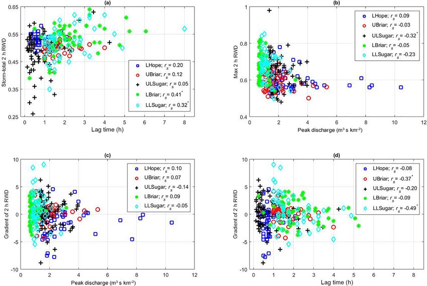
418           M. ten Veldhuis et al.: The role of storm scale, position and movement in controlling urban flood response

ization on peak flows and response times, associated with           Analysis (GSSHA) model to examine the effect of rainfall
a combination of imperviousness and flood mitigation mea-           time and length scales on flood response. They found that
sures, especially for basins where urbanization has predom-         peak flows in the larger basins (∼ 50–100 km2 ) were domi-
inantly taken place after implementation of stormwater con-         nated by large-scale storms, while more concentrated orga-
trol legislation (e.g. Smith et al., 2013a; Hopkins et al., 2015;   nized thunderstorm systems dominated in the smaller basins
Miller et al., 2014). Niemczynowicz (1999) and Schilling            (∼ 7–30 km2 ). They also identified limitations of this and
(1991) pointed out the importance of spatially distributed          similar modeling studies, where hydrologic response may be
rainfall information at high resolution to study response in        attributable to errors in radar rainfall estimates or to features
urban basins. Thanks to the advances of weather radar, such         that were omitted or poorly represented in the model, such as
information is becoming increasingly available (Krajewski           detention ponds, the spatial distribution of layered soils and,
and Smith, 2002; Berne and Krajewski, 2013), typically at           in particular, initial soil moisture.
1 km spatial resolution (Smith et al., 2007), and in some cases        Smith et al. (2002) used a data-driven approach to study re-
down to less than 100 m (Otto and Russchenberg, 2011; Chen          lationships between temporal and spatial rainfall variability
and Chandrasekar, 2015; Thorndahl et al., 2017). (Wright            and hydrological response in urban basins. They introduced
et al., 2014b) analyzed flow variability in three suburban-         the concept of rainfall-weighted flow distance, representing
ized catchments in relation to different radar rainfall prod-       storm position and movement relative to the flow-path net-
ucts and found that storm event water balance and hydrolog-         work in the basin. In their study, they analyzed hydrological
ical response times varied with the radar product used for          response in five semiurbanized basins in the US for five ex-
analysis. Berne et al. (2004) derived relationships for critical    treme flood-producing storms based on detailed radar rain-
rainfall resolution for urban hydrology, using high-resolution      fall and flow observation datasets. They found that fractional
radar rainfall datasets over six basins in the Mediterranean        coverage of a basin by heavy rainfall is a key element of
region. They found that the temporal and spatial rainfall res-      scale-dependent flood response: storm event scales, i.e. spa-
olution required for urban hydrological analysis varied from        tial (area, length) and temporal (duration) scales smaller than
about 5 min, 3 km for basins ∼ 10 km2 , to about 3 min, 2 km        the basin scale (basins length, response time), lead to lower
for basins of ∼ 1 km2 scale. Radar rainfall data have been          runoff ratios and flood peak compared to when scales of rain-
used in various studies in recent decades to drive hydrologi-       fall and basin are similar. Storm motion was found to be am-
cal models and sensitivity of urban hydrological response to        plifying peak flow under particular conditions: storm motion
spatial and temporal rainfall variability. Bruni et al. (2015)      from the lower basin to the upper basin on a timescale of ap-
and Ochoa-Rodriguez et al. (2015) used rainfall data from           proximately 2 h served to amplify peak discharge for the case
a polarimetric rainfall radar, at ∼ 30–100 m and minute res-        of a large, ∼ 100 km2 basin, relative to other modes of storm
olution to drive semidistributed hydrodynamic models of             motion. In Smith et al. (2005), spatial rainfall variability in
one and seven highly urbanized catchments, respectively, in         relation to the flow-path network was analyzed for 25 flash-
northwestern Europe to study urban hydrological response            flood-producing storms in a 14 km2 urban watershed. They
for a range of rainfall input resolutions. They found that sen-     found that spatial rainfall variability was strongly smoothed
sitivity of flows to rainfall variability increased for smaller     by the flow-path network, resulting in hydrological responses
basin sizes and that hydrological response was more sensi-          for storms with widely varying spatial rainfall variability be-
tive to change in temporal than in spatial rainfall input res-      ing strikingly similar.
olution. Gires et al. (2012) quantified the impact of unmea-           Other authors have used similar concepts to study hydro-
sured small-scale rainfall variability on urban runoff for an       logical response in natural basins. In an extensive study of
urban catchment in London, by downscaling radar rainfall            300 events over a 148 km2 basin in Arizona, Syed et al.
data from 1 km and 5 min resolution to a resolution 9–8 times       (2003) found that runoff volume and peak were strongly cor-
higher in space and 4–1 times higher in time. Uncertainty in        related with areal coverage by the storm core (> 25 mm h−1
simulated peak flow associated with small-scale rainfall vari-      rainfall intensity). The importance of the storm core’s posi-
ability reached 25 and 40 % respectively for frontal and con-       tion increased with basin size, with storm cores positioned in
vective events. Rafieeinasab et al. (2015) analyzed sensitivity     the central portion of the watershed producing more runoff
of hydrological response to rainfall variability for five urban     and higher flood peaks. Morin et al. (2006) found that the
catchments of different sizes, located in the City of Arling-       sensitivity of flood response (in terms of flood peak mag-
ton and Grand Prairie (US), using a distributed hydrologi-          nitude and peak timing) to spatial rainfall variability in-
cal model. They found that while flow variability was better        creased with storm intensity, which they attributed to high
captured using higher resolution rainfall input, errors in re-      flow velocities during intense storms. Similar results were
producing flow by the models remained equally large, with           found by Lobligeois et al. (2014), who analyzed the influ-
peak flow over- and underestimations of more than 100 %.            ence of spatial rainfall variability on hydrological response
   (Wright et al., 2014a) analyzed hydrological response for        in 181 catchments in France based on spatial rainfall vari-
four semiurbanized basins in Charlotte watershed, North             ability, storm position and catchment-scale storm velocity
Carolina, using a Gridded Surface Subsurface Hydrologic             indices. They found that flow simulations by hydrological

Hydrol. Earth Syst. Sci., 22, 417–436, 2018                                        www.hydrol-earth-syst-sci.net/22/417/2018/
M. ten Veldhuis et al.: The role of storm scale, position and movement in controlling urban flood response                      419

models benefited from spatially distributed rainfall input for       (USGS) in 1995. We analyze the influence of spatial scale,
large catchments and strongly spatially distributed rainfall         position and movement of storms relative to the flow-path
fields. Nicotina et al. (2008) analyzed rainfall variability in      network as well as interactions with spatial distribution of
a numerical study for large basins up to several thousand            imperviousness on urban flood response. We aimed to ad-
square kilometers and found that spatial variability of a storm      dress the following questions.
was more important than variability in total rainfall volume
over the basins. This was attributed to the dominant influence           – How does rainfall scale interact with basin scale in de-
of hillslope flow on scales typically smaller than the rainfall            termining urban flood response? We use fractional cov-
variability scale, smoothing differences in travel times to the            erage to express the relation between rainfall scale and
basin outlet. Channel flow only became more important in                   basin scale and to investigate the dependencies of flood
very large basins (> 8000 km2 ), leading to stronger sensitivity           peak magnitude and lag time on rainfall scale.
to spatial rainfall variability. Zoccatelli et al. (2011) analyzed
                                                                         – Does the position of a storm in relation to the flow-path
rainfall coverage, storm position and movement relative to
                                                                           network influence flood response? We use the concept
the flow-path network for five storms in five different basins
                                                                           of rainfall-weighted flow distance (RWD) to identify the
in southeastern Europe. Based on a model sensitivity study,
                                                                           position of a storm relative to the flow-path network and
they found that peak timing error introduced by neglecting
                                                                           analyze whether storms concentrated in the upstream
spatial rainfall variability ranged between 30 and 72 % of the
                                                                           part of the catchment are associated with significantly
corresponding catchment response time. Nikolopoulos et al.
                                                                           different responses compared to storms concentrated in
(2014) analyzed the role of storm motion using radar rainfall
                                                                           the center or near the basin outlet.
data to drive two models of varying complexity. They found
that storm motion did not play a significant role in generating          – How does storm direction and velocity in relation to
hydrologic response for a large storm event, in basins sized               the flow-path network influence flood response? We use
8–623 km2 . Emmanuel et al. (2015) investigated the impacts                first-order differences in RWD to characterize storm
of spatial rainfall variability on hydrological response using a           movement and investigate if storms passing over the
model simulation approach and found significant dispersion                 basin in the downstream direction lead to significantly
in results obtained for events for different simulation scenar-            different hydrological responses compared to storms
ios, showing the need for studying larger sets of events to                moving in the upstream direction and storms moving
derive robust general conclusions. Modeling studies reported               perpendicular to the main flow direction.
in the literature have remained inconclusive with respect to
the interactions between rainfall and catchment scales (Og-              – How does the position of a storm in relation to the spa-
den et al., 2011; Morin et al., 2006; Nicotina et al., 2008;               tial distribution of imperviousness influence flood re-
Rafieeinasab et al., 2015). This emphasizes the importance                 sponse?
of using field observations to corroborate preliminary con-
                                                                        This paper is organized as follows: in Sect. 2, the case
clusions drawn from model simulations.
                                                                     study area, datasets and methods used in this study are in-
   In this study, we extracted a catalog of 279 flood events
                                                                     troduced. Results are presented and discussed in Sect. 3, fol-
from 15 years of high-quality flow observations, in five
                                                                     lowed by summary and conclusions in Sect. 4.
nested (semi)urbanized basins in Charlotte region, North
Carolina (US). By flood events we understand the set of
events associated with the top five largest peak flows per           2     Data and methods
year, on average. The term “flood response” is used to re-
fer to hydrological response associated with these high flow         2.1    Study region, rainfall and flow datasets
events, on the (sub)catchment scale. In the catchments we
investigated, it is hard to distinguish between “bank-full”          The data used in the study were collected at five USGS
flow and inundating flows, since channels and natural flood-         stream gauging stations in Charlotte-Mecklenburg county,
plains were heavily modified as a consequence of urbaniza-           North Carolina. Gauging stations are located at the outlet of
tion. As a result, what used to be considered bank-full flow         hydrological basins that range from 7.0 to 111.1 km2 in size.
in a natural channel could be considered flooding (of pri-           The area is largely covered by low- to high-intensity urban
vate properties, gardens) in the urbanized context (Turner-          development, covering 60 to 100 % of basin areas. The per-
Gillespie et al., 2003). Observational resources for the Char-       centage of impervious cover varies from 25 % in the least
lotte metropolitan region are exceptionally rich (e.g. Smith         developed to 48 % in the most urbanized basin covering the
et al., 2002; Wright et al., 2013). The region is covered by         city center of Charlotte. Figure 1 shows a map with the loca-
two National Weather Service WSR-88D (Weather Surveil-               tion of the area, catchment boundaries and location of stream
lance Radar-1988 Doppler) radar instruments, both of which           gauges used in the analysis. High-resolution (30 m) grid-
were deployed in 1995. A dense network of rain gauges and            ded datasets were used for terrain elevation (National Map
stream gauges was installed by the US Geological Survey              of USGS, http://viewer.nationalmap.gov/), impervious cover,

www.hydrol-earth-syst-sci.net/22/417/2018/                                           Hydrol. Earth Syst. Sci., 22, 417–436, 2018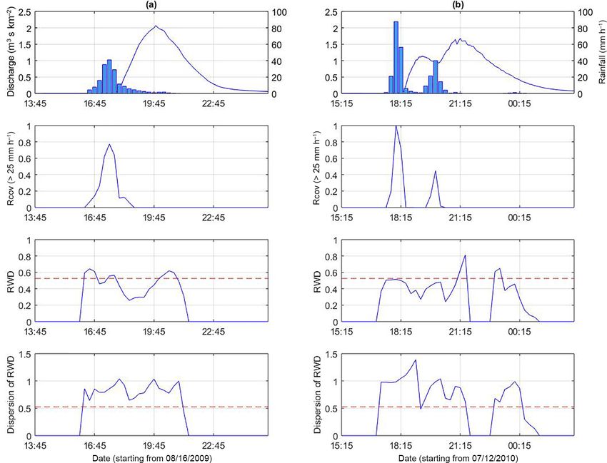
420            M. ten Veldhuis et al.: The role of storm scale, position and movement in controlling urban flood response

Figure 1. Location of Little Sugar Creek catchment (c), topography (a), land use and land cover (b), and location and boundaries of subbasins,
including locations of flow gauges and the location of rainfall radar.

land use and land cover (LULC, from National Land Cover                  ered by the urban core of the city of Charlotte. Upper and
Dataset NLCD, available at: http://www.mrlc.gov/).                       lower Briar (hereafter Upper Briar and Lower Briar) are
   The focus of this was Little Sugar Creek catchment, up-               the least urbanized basins, with impervious cover of 23.9
stream of the flow gauge at Archdale, with a total drainage              and 24.7 % respectively; Little Hope (LHope) is the small-
area of 111 km2 . Additionally, we used data from basins                 est basin in size. Maximum flow distance along the flow-path
nested within the main basin, sized 7.0, 13.3, 31.5 and                  network varies from 49 km for the smallest to 213 km for the
48.5 km2 . Stream gage data were collected at 5 to 15 min in-            largest basin. Basin compactness, computed as the ratio of
tervals over the period 2001–2015. For this study, all flow              basin area over perimeter squared, is highest for Little Hope
data were linearly interpolated 1 min values and converted to            and lowest for Upper LSugar, showing that the latter is the
UTC time. Gauges measure water depth using pressure trans-               most elongated basin. Dams have been implemented in three
ducers, using an accuracy standard set by the USGS Office                of the basins, all for recreational purposes, according to the
of Surface Water for stage measurement at approximately                  National Inventory of Dams (nid.usace.army.mil/cm_apex).
0.01 foot (ft) or 0.2 percent of the effective stage. Flows are          Storage volume varies from approximately 0.1 to 2 mm (dam
derived from stage–discharge curves that were established                storage volume divided by basin area).
based on protocols developed by USGS and include man-                       Based on data from the USGS flow datasets, we es-
ual flow measurements during site visits performed by USGS               tablished a catalog of flood events, based on “peak-over-
staff. As part of this procedure, stage–discharge curves are             threshold” selection such that we have, on average, five
checked and recalibrated during site visits several times per            events per year over the period 2001–2015. Since radar rain-
year. More information on gauge data and field measure-                  fall data were only available for the summer season, April to
ments is available at http://waterdata.usgs.gov/nc/nwis. Flow            September, events were extracted exclusively for this period.
datasets for the Charlotte region are of exceptionally high              Flood events are local maxima in discharge for which there
quality and consistency as data collection protocol and gauge            is not a larger discharge in a time window of 12 h centered on
locations have remained unchanged over decades.                          the peak time. Events with incomplete rainfall or discharge
   A summary of basin characteristics in Little Sugar Creek              data were excluded from the dataset. This resulted in a cata-
catchment is provided in Table 1. (Sub)basin areas range                 log of 50 to 69 storm events per basin (see Table 1).
from 7.0 to 111.1 km2 , with impervious cover from 23.9 to                  Rainfall amounts were computed for the time period as-
48.2 % and urban land use (excluding parks and lawns) cov-               sociated with each of the flood events, based on radar rain-
ering 47.1 to 79.1 % of the basin area. Upper Little Sugar               fall data. A total of 15 years (2001–2015) of high-resolution
(Upper LSugar hereafter) is the most urbanized basin, cov-               (15 min, 1 km2 ) Hydro-NEXRAD radar rainfall fields were

Hydrol. Earth Syst. Sci., 22, 417–436, 2018                                               www.hydrol-earth-syst-sci.net/22/417/2018/

M. ten Veldhuis et al.: The role of storm scale, position and movement in controlling urban flood response                                   421

Table 1. Summary of hydrological basins in the Little Sugar Creek catchment: basin area (km2 ), imperviousness (%), slope (–), land use
coverage (high intensity, medium intensity, low intensity urban development) (%), maximum flow distance (km), number of dams regulating
stormwater flows (–), number of POT flood events used for analysis (–).

    Name           USGS         Drainage   Slope   Max. flow   Basin com-     Impervi-         Land use coverage (%)       No. of   No. of
                   ID               area            distance     pactness      ousness     high int. med. int. low int.     dams    events
                                  (km2 )     (–)    (km) (–)          (%)                                                     (–)      (–)
    Little Hope    02146470          7.0     2.2         49           2.6         32.2            9.3         9.4   48.5       0       54
    Upper          0214642825       13.3     1.9         58           2.3         23.9            3.6         9.3   34.2       1       50
    Briar
    Upper          02146409         31.5     2.2        128           1.4         48.2           22.5         24    32.6       0       69
    Little Sugar
    Lower          0214645022       48.5     2.4        168           1.6         24.7            4.5         9.9   32.8       5       54
    Briar
    Lower          02146507        111.1     2.4        213           1.6         32.0           10.3        14.1   32.8       8       52
    Little Sugar

available for this study, based on volume scan reflectivity            smooth some of the rainfall variability, especially for fast-
observations from the NWS-operated Weather Surveillance                moving storms, they sufficiently capture the rainfall infor-
Radar 1988 Doppler (WSR-88D) radar in Greer, South Car-                mation relevant for this study, i.e. minimum, mean and max-
olina (radar code KGSP, see Fig. 1c). The Hydro-NEXRAD                 imum distance of storms relative to the outlet and movement
processing system was developed to generate radar rainfall             of storms relative to the flow-path network.
estimates for hydrologic applications by converting three-
dimensional polar-coordinate volume scan reflectivity fields           2.2     Methods
from NWS WSR-88D radars into two-dimensional Carte-
sian surface rainfall fields (Krajewski et al., 2011). The             2.2.1     Hydrograph and basin average rainfall
standard convective rainfall–reflectivity (Z–R) relationship                     characteristics
(R = aZ b , where a = 0.017, b = 0.714; R is rain rate in
                                                                       The following rainfall metrics were defined per event, based
millimeters per hour, Z is radar reflectivity in millimeters
                                                                       on basin-average rainfall rates derived from radar rainfall
to the power six per cubic meter), a 53 dBZ hail threshold,
                                                                       data at 15 min, 1 km2 resolution.
and several standard quality control algorithms are used (see
Seo et al., 2011 for more details). No range correction al-                 – Basin-average rainfall rate (mm h−1 ):
gorithms are used in this study. The dataset has been exten-
sively validated in Wright et al. (2014b) and used for rain-
fall frequency analysis in Wright et al. (2013). Mean field                                ZT
bias correction of the radar rainfall is done on the daily scale               Rb (t) =         R(t, x)dx,                                   (1)
using 71 rain gages from the Charlotte rain gauge network                                  0
(CRN) (see Wright et al., 2014b). Radar-based rainfall esti-
mates captured rainfall variability on timescales of 5–15 min                  where Rb (t) is the basin-average rainfall rate at times t
based on the sampling resolution of the radar beam, and                        (mm h−1 ); R(t, x) is the rain rate at pixel x (1 × 1 km2 )
space scales of 1 km2 . We used rainfall data at a temporal                    at time t (time step is 15 min), and T is the time period
resolution of 15 min to avoid sensitivity to sampling error on                 of the selected event, from 12 h before the time of the
the 5 min timescale. Radar rainfall data were spatially resam-                 maximum peak flow for a storm event until 12 h after
pled at 30 m resolution using inverse-distance interpolation                   the time of peak flow.
between radar pixel centroids, to enable computation of rain-
                                                                            – Rainfall duration Rd (hours), duration of rainfall above
fall redistribution relative to the flow-path network and im-
                                                                              a minimum threshold of 1 mm h−1 within the rainfall
perviousness, within the radar pixel (as will be explained in
                                                                              event:
the next section). Basin-average rainfall rates were also com-
puted, based on spatial aggregation of rainfall values over                           ZT
1 km2 pixels within the catchment boundaries of the individ-                   Rd =        I (Rb (t) > 1) dt, where I (Rb (t, x) > 0)
ual basins (percent of each 1 km2 grid in the basin was com-
                                                                                      0
puted for pixels overlapping catchment boundaries). While
                                                                                           1 for Rb (t, x) > 1 mm h−1

15 min estimates derived from 5 min radar sampling may                            =                                                          (2)
                                                                                           0 otherwise.

www.hydrol-earth-syst-sci.net/22/417/2018/                                                     Hydrol. Earth Syst. Sci., 22, 417–436, 2018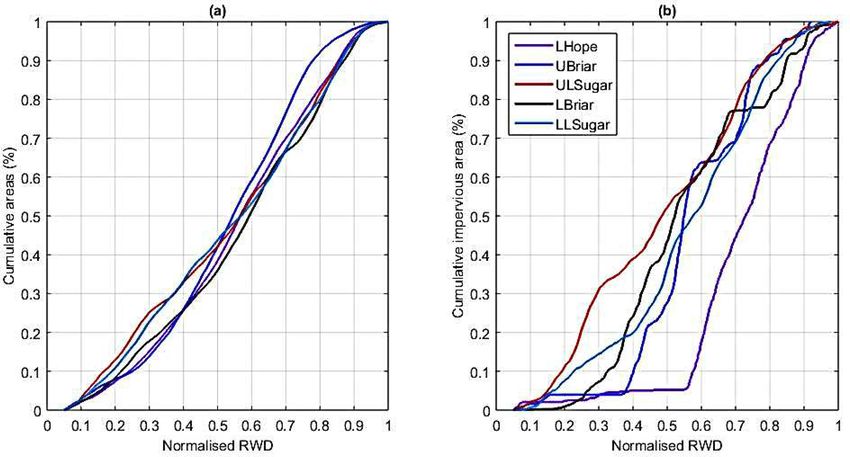
422                M. ten Veldhuis et al.: The role of storm scale, position and movement in controlling urban flood response

  – Total rainfall depth per event (mm):                              – Lag time (hours): Tl , defined as the time difference be-
                                                                        tween basin-average rainfall peak and maximum peak
                                                                        flow, computed from the time distance between the time
                   ZT                                                   of peak flow and time of basin-average maximum rain-
      Rb,tot =          Rb (t).                             (3)         fall intensity during the preceding 12 h time period. In
                                                                        our initial analyses, we used two methods to compute
                   0
                                                                        lag times, based on peak-to-peak and on distance be-
                                                                        tween centroids of hyetograph and hydrograph. The lat-
  – Maximum 15 min rainfall intensity (mm h−1 ):                        ter resulted in a large number of negative lag time val-
                                                                        ues, associated with events with multiple rainfall and/or
                                                                      peak flows. After visual inspection of hyetographs and
      Rb,max = max Rb (t) : t ∈ [0, T ] .                   (4)         hydrograph peaks, we decided that peak-to-peak time
                                                                        gave a better representation of the response between
                                                                        rainfall and peak flows for most events, and hence we
  The following metrics were used to analyze relationships              decided to stick to this lag time definition in our analy-
between rainfall and hydrologic response; flow values were              ses.
normalized by basin area and expressed in cubic meters per
                                                                      – Runoff ratio (–): normalized runoff divided by total
second per square kilometer (m3 s−1 km−2 ), to allow com-
                                                                        basin-average rainfall over the duration of the flood
parison among different basins.
                                                                        event (TQ ).
  – Maximum normalized peak flow (m3 s−1 km−2 ):                      – Peak ratio (–): normalized peak flow (flow divided by
                                                                        basin area) divided by rainfall peak intensity.
                                                                 2.2.2   Rainfall spatial characteristics: spatial
                      −1
      Qmax = max Q(t)A : t ∈ [0, T ] ,                      (5)            variability, fractional coverage and
                                                                           rainfall-weighted flow distance
      where Q is the instantaneous flow observation, at 1 min      We used fractional coverage of the basin by rainfall above a
      intervals (m3 s−1 ); A is the basin area (km2 ).             given threshold to analyze the influence of rainfall scale in re-
                                                                   lation to basin scale on hydrological response. Additionally
                                                                   we used the concept of rainfall-weighted flow distance, as
  – Total normalized runoff volume (m3 ):
                                                                   first introduced by Smith et al. (2002). RWD provides a rep-
                                                                   resentation of rainfall variability relative to a distance met-
                                                                   ric imposed by the flow-path network. The methodology has
               ZT                                                  been used in multiple previous studies (Smith et al., 2002,
      Qtot =           Q(t)A−1 dt.                          (6)    2005; Zoccatelli et al., 2011; Nikolopoulos et al., 2014; Em-
               0                                                   manuel et al., 2015). It represents the position of a storm
                                                                   relative to the flow-path network and is used to analyze
  – Flood event duration (hours): TQ , defined as the              how storm position and movement influence hydrological re-
    interval between the time when the unit hydro-                 sponse.
    graph continuously rises above 0.05 and falls below               Rainfall fractional coverage (–) was computed as follows:
    0.01 m3 s−1 km−2 . Thresholds were established based                          Z
    on visual inspection of the hydrographs and work well                          1
                                                                   Rc (t) = max        I (R(t, x)) dx ,                          (7)
    for flood events with a single peak (or events separated                       A
                                                                                     A
    from other flood peaks by at least 6 h). For flood events
    with multiple peaks (i.e. flood peaks that are either pre-     where I (R(t, x)) is the indicator function and equals 1 when
    ceded or followed by another flood peak within a short         R(t, x)>r or 0 otherwise; Rc (t) is the maximum portion of
    time, e.g. 1 h), these thresholds can result in anoma-         basin area receiving rainfall equal to or exceeding r mm h−1
    lously long event durations that are not representative        rainfall. We used a threshold of r = 25 mm h−1 , represen-
    of hydrological response behavior. For these events, we        tative of high-intensity rainfall. This threshold corresponds
    manually determined the start and end time for each of         with the 1 in threshold that is used by the flood hazard com-
    the “multi-peak” events by visually inspecting the hy-         munity in US, specifically the National Weather Service, as
    drographs. We further checked the duration for “single-        an index for potential flash flooding. It has also been used
    peak” events through visual inspections, to ensure con-        previously in the literature to investigate the influence of
    sistency in the definition of event duration.                  storm core versus overall rainfall (e.g. Syed et al., 2003).

Hydrol. Earth Syst. Sci., 22, 417–436, 2018                                       www.hydrol-earth-syst-sci.net/22/417/2018/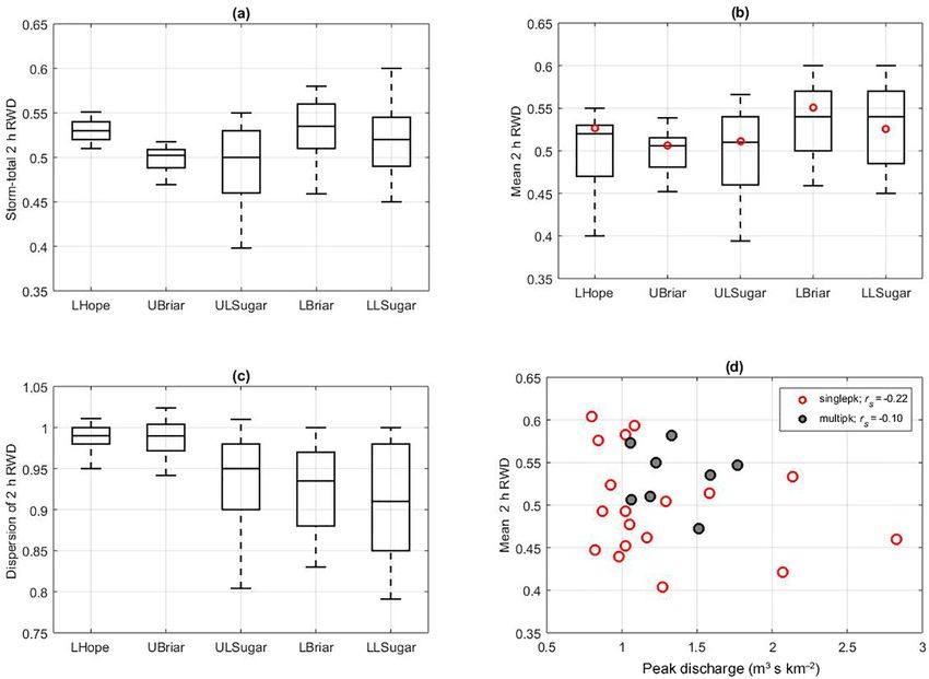
M. ten Veldhuis et al.: The role of storm scale, position and movement in controlling urban flood response 423
Rainfall-weighted flow distance (RWD(t), in m) was com- RWD dispersion takes the value 1 for uniform rainfall;
puted as follows: values below 1 are associated with unimodal spatially dis-
Z tributed rainfall and values above 1 represent multimodal
RWD(t) = w(t, x)d(x)dx, (8) spatially distributed rainfall peaks in relation to the flow-path
network.
A
To further investigate the influence of spatial distribution
where distance function {d(x); x ∈ A} is the flow distance of urbanization on urban flood response, we computed nor-
from point x within the basin to the outlet of the basin and malized RWD strictly for pixels with impervious cover larger
w(t, x) is the rainfall weight function: than 80 %, classified as high-intensity development in the
NLCD dataset. Thus, imperviousness-weighted, normalized,
R(t, x)
w(t, x) = R R(t, x)dx. (9) rainfall-weighted flow distance (DI (t)) was computed as fol-
A lows:
RWD is normalized by maximum flow distance in the net- 1
Z
work, as follows: DI (t) = I (x)w(t, x)d(x)dx, (14)
dmax
Z A
1
D(t) = w(t, x)d(x)dx, (10)
dmax where I (x) is an impervious indicator and takes value 1 for
A pixels with impervious cover > 80 % and 0 for pixels with
where D(t) is the rainfall-weighted flow distance, normal- impervious cover < 80 %.
ized by maximum flow distance (–), dmax = {d(x); x ∈ A},
2.2.3 Summary statistics and correlation analysis
maximum flow distance in the flow-path network (m).
The random variable D(t) takes values from 0 to 1: low Metrics associated with normalized RWD are sensitive to the
values of D(t) are associated with rainfall that is spatially length of the time window over which they are computed
concentrated near the outlet, high values with rainfall con- (Smith et al., 2002; Nikolopoulos et al., 2014). We used a
centrated near the headwaters of the basin. For uniformly range of time windows of x h rainfall, x varying from 0.5 to
distributed rainfall, all weights across the basin are equal and 3 h, corresponding to the timescales of storm duration and lag
D(t) represents the mean flow distance imposed by the flow- time for the largest two basins (median storm durations 3 and
path network: 3.5 h, median lag times 1.7 and 2.0 h respectively). Results
Z based on a 2 h window are shown in Sect. 3. The time win-
d = d(x)dx. (11) dow was centered over the time of event-maximum rainfall
A intensity. The following summary statistics were retained for
normalized RWD: mean, minimum, maximum, coefficient
Normalized, rainfall-weighted flow distances were com-
of variation (CV) and gradient as well as RWD for event-
puted per time step as well as for the total accumulated rain-
total accumulated rainfall. We analyzed time-varying spa-
fall per storm event. The first provides information on storm
tial coverage by the storm core (> 25 mm h−1 ), 1Rcov /1t,
movement over the basin relative to the flow-path network
in relation to basin-average rainfall 1R/1t to see how much
and combines both temporal and spatial rainfall variation
of change in rainfall intensity is associated with change in
(Smith et al., 2002), while the latter focuses on the spatial
storm core coverage of the basin. We analyzed 1R/1t ver-
aspect of rainfall distribution, summarizing it for the total
sus 1RWD/1t to see how change in rainfall intensity relates
accumulated rainfall per storm event (Smith et al., 2005).
to movement of the storm relative to the flow-path network.
RWD dispersion was computed, to provide an indication
Correlation analyses were performed for all combinations of
of whether spatial rainfall variability as imposed by the flow-
metrics associated with basin-average rainfall, flow hydro-
path network is unimodal or multimodal. The normalized
graph, spatial rainfall variability and imperviousness distri-
RWD dispersion (–) was defined as follows (Smith et al.,
bution, based on Spearman rank correlations. Correlations
2005).
were tested for significance at the 5 % level (p value > 0.05,
Z
1
2
based on t test).
1 2
S(t) = w(t, x) d(x) − d dx (12)
s
A 3 Results and discussion
where s is the dispersion for uniform rainfall: 3.1 Rainfall and hydrograph characteristics of the
1 selected events
Z 2 2
s= d(x) − d dx . (13) In Fig. 2, box plots of rainfall and flow characteristics are
shown for the catalog of selected events, for the five basins.
A
www.hydrol-earth-syst-sci.net/22/417/2018/ Hydrol. Earth Syst. Sci., 22, 417–436, 2018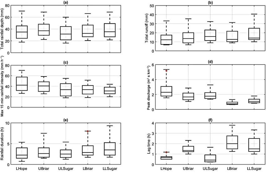
424            M. ten Veldhuis et al.: The role of storm scale, position and movement in controlling urban flood response

Figure 2. Box plots showing 10, 25, 50, 75 and 90 % quantiles of characteristic rainfall and flow values for all events, per basin: total basin-
average rainfall depth (a), total normalized runoff volume (mm) (b), max 15 min rainfall intensities (mm h−1 ) (c), normalized peak flows
(m3 s−1 km−2 ) (d), rainfall duration in hours (e), lag time (f). Box plots are based on 50 to 69 events per basin, as listed in Table 1.

The plots show that basin-average rainfall depth was of the               ative to its basin size and quantile ranges similar to the much
same order of magnitude for all basins, with median val-                  smaller UBriar basin. This is confirmed by coefficient of vari-
ues varying between 32.2 and 37.0 mm. Runoff volumes are                  ation values of the flow distributions per basin: 0.37 and 0.
slightly lower for the smallest two basins in terms of their              46 for Upper and Lower LSugar; 0.65, 0.46 and 0.44 for
median values and less skewed. Peak rainfall intensities show             LHope, Upper and Lower Briar. Similar results were found
stronger variation with basin size: median for peak 15 min                for a wider range of basins in this region in (Ten Veldhuis
rainfall intensity decreases from 41.7 mm h−1 for the small-              and Schleiss, 2017), who concluded that for the basins in the
est to 31.2 mm h−1 for the largest basin. Peak rainfall in-               Charlotte catchment, flow regulation and peak flow restric-
tensity varied by factor of 10 approximately across the set               tions induced by capacity constraints result in an overall ef-
of selected peak events per basin (9.5 to 87.6 mm h−1 for                 fect of peak flow reduction associated with urbanization. The
Lower LSugar; 9.3 to 83.2 mm h−1 for Lower Briar; 9.7                     only quantitative information available to us about stormwa-
to 91.7 mm h−1 for Upper LSugar; 8.8 to 90.7 mm h−1 for                   ter infrastructure in the Charlotte catchment is the number of
Upper Briar; 10.4 to 118.5 mm h−1 for LHope). Figure 2d                   dams, which is low for all 5 catchments (0, 1, 0, 5 and 8 for
shows large differences in peak flows between the basins,                 the smallest to largest catchment). In a recent study by (Bell
as indicated by 25–75 and 10–90 % ranges per basin. Lower                 et al., 2016), additional information was collected for basins
Briar has lowest median normalized peak flows and narrow-                 in this region. They computed the percentage area of miti-
est quantile ranges, tied to a combination of large area size             gated area by detention structures: 5.5, 5.8 and 3.2 % for Lit-
and low impervious cover compared to other basins, result-                tle Hope, Upper Briar and Upper Little Sugar, respectively.
ing in strongly smoothed flood response. The smallest basin,              These numbers show that the impact of detention structures
LHope, has a strongly skewed peak flow distribution, with                 on hydrological response is likely to be very small.
the highest median as well as the largest quantile ranges of                 Flow peaks for our event catalog (maximum flow peaks
normalized peak flow values compared to the other basins.                 per basin were 3.4 and 10.4 m3 s−1 km−2 , respectively) were
The lowest flow variability is found for the most urbanized               associated with 100-year return periods in 1990 and 1992,
basin (size 31.5 km2 ), which suggests a smoothing effect of              respectively, decreasing to 8 and 20 years in 2007, following
imperviousness on flow variability. Upper LSugar, the most                (Villarini et al., 2009), who reported flood frequency distri-
impervious basin, shows a high median peak flow value rel-                butions for Lower LSugar Creek and for LHope Creek, based

Hydrol. Earth Syst. Sci., 22, 417–436, 2018                                                www.hydrol-earth-syst-sci.net/22/417/2018/
M. ten Veldhuis et al.: The role of storm scale, position and movement in controlling urban flood response                    425

on a generalized additive model fitted to annual flood peaks      Additionally, spatially varied rainfall data include far more
in these 2 basins. For rainfall, we compared return inter-        zero values, which leads to strongly skewed distributions, as
vals of maximum 15 min rainfall intensities (over 1 × 1 km2       is confirmed by large differences between mean and median,
with point rainfall frequency estimates provided by NOAA          while these differences are small for temporal rainfall vari-
(NOAA, 2017); no frequency estimates were available on a          ability. Still, these results show that rainfall for the selected
1 × 1 km2 scale. Maximum values per event varied from 8.8.        flood events tends to be highly spatially variable. Moreover,
to 132 mm h−1 , associated with return intervals of less than     spatial variability changes over the duration of events, more
1 year up to 25 years on the point scale.                         strongly so for the larger than for the smaller basins. This
   Rainfall duration varied from approximately 0.5 to 14 h,       is a characteristic of hydroclimatic conditions in this region
representing a wide range from concentrated, single-peak          northeast of the Appalachians, as confirmed for instance by
events to prolonged, multi-peak events (Fig. 2e). Distribu-       Zhou et al. (2017). Similar results were found by Lobligeois
tions show large quantile ranges (2.5 to 4 h, 25–75 % range)      et al. (2014), who analyzed spatial variability of storm events
and are highly skewed. Values in the upper percentiles were       associated with the largest 20 flood events in 181 basins
mainly associated with storm events with multiple rainfall        in France. They showed that spatial rainfall variability was
peaks. Lag times (Fig. 2f), computed as time between max-         strongly dependent on hydroclimatic regions, with high vari-
imum rainfall intensity and peak flow, are strongly tied to a     ability occurring in the Mediterranean area, associated with
combination of basin area size and impervious cover. Upper        summer convective storms, and low variability over much of
LSugar, the most urbanized basin, has the shortest median lag     the northern and western regions of France.
time (26 min); the two largest basins have median lag times          Figure 3 shows box plots and empirical histograms of
of 1.7 and 2 h, whereas Lower LSugar has a slightly shorter       fractional rainfall coverage, i.e. the maximum percentage
median lag time than Lower Briar, despite its larger size. This   of basin area covered by rainfall intensities larger than
confirms findings in an earlier study by Smith et al. (2002),     25 mm h−1 during storm events, representing the most in-
who found that peaks at Lower LSugar are mostly linked            tense core of the storm. The box plots show that storm cores
to discharge from the highly urbanized Upper LSugar basin.        exceed basin scale for 43 and 23 % of the storms in the
Lag time values in the upper percentiles are generally asso-      two smallest basins (7 and 13.3 km2 , respectively). For the
ciated with multi-peak events, where multiple rainfall peaks      larger basins this decreases to 10, 4 and 2 % (for basin sizes
caused one or more peak flows over a prolonged period of          31.5, 48.5 and 111.1 km2 , respectively). Similar results were
time. Runoff ratios vary mainly with imperviousness degree:       shown by Smith et al. (2002) and Syed et al. (2003) for the
the largest median runoff ratio was found for Upper LSugar        same range of (sub)basin sizes, for 5 storms using radar rain-
(0.51), followed by Lower LSugar (0.44), Lower Briar (0.38)       fall data and for 300 summer storms in Arizona using in-
and the two smallest basins, Upper Briar (0.35) and LHope         terpolated rain gauge data, respectively. Another interesting
(0.34). Variability in runoff ratio, expressed in terms of co-    feature appears in the empirical histograms: for the smaller
efficient of variation, is low for Upper and Lower LSugar         basins, fractional coverage values tends to be either small
basins compared to the other basins (figure not shown). This      compared to basin size (coverage 0–20 %) or approaching
effect is even stronger for peak-to-peak ratios: variability in   basin size (coverage 80–100 %). Zhou et al. (2017) showed
terms of CV is very low for the more impervious basins (0.5       that the hydro-climatology of flood events in this region re-
and 0.6 respectively for Upper and Lower LSugar) compared         flects a mixture of flood agents, consisting of thunderstorms
to the other basins (CV values 5.1, 4.2 and 3.7 for LHope,        and tropical cyclones. The largest fraction of events in the
Upper and Lower Briar, respectively).                             upper tail of flood distributions for basins in this area is
                                                                  associated with organized thunderstorms, which could ex-
3.2   Spatial rainfall variability and fractional basin           plain the spatially concentrated nature of storm cores over
      coverage                                                    LSugar Creek subbasins. Table 2 shows the degree of over-
                                                                  lap in selected storm events between the five (sub)basins. The
Spatial rainfall variability was analyzed based on the coeffi-    table shows that 54 to 69 % of events in the largest basin
cient of variation of rainfall intensities per time step. Mean    (Lower LSugar) is represented in the flood event catalog for
CV values vary from 1.24 for the smallest to 3.51 for the         the smaller basins (first row), indicating that these events
largest basin, showing that rainfall tends to be more spatially   are likely to have been large-scale events, affecting the en-
uniform for smaller basins compared to larger basins. Spa-        tire basin. Overlap between flood-producing events in Upper
tial variability is high compared to temporal rainfall vari-      Briar and Lower Briar is 59 %. The lowest overlap occurs for
ability based on basin-average rainfall, where CV values          LHope, indicating that a substantial part of flood events in
vary between 0.94 and 1.03 (no clear relation with basin          this smaller basin is associated with a different collection of
size). This is partially a result of the difference in aggre-     storm events compared to the other basins. As we can see
gation scales: basin-average rainfall is aggregated over 7 to     in Fig. 2, a higher degree of overlapping storms between
111 km2 and 15 min, while spatially variable rainfall is ag-      basins does not result in more similar rainfall or flow pat-
gregated over 1 km2 and several hours of rainfall duration.       terns: rainfall and flow characteristics are as similar or dis-

www.hydrol-earth-syst-sci.net/22/417/2018/                                        Hydrol. Earth Syst. Sci., 22, 417–436, 2018
426 M. ten Veldhuis et al.: The role of storm scale, position and movement in controlling urban flood response
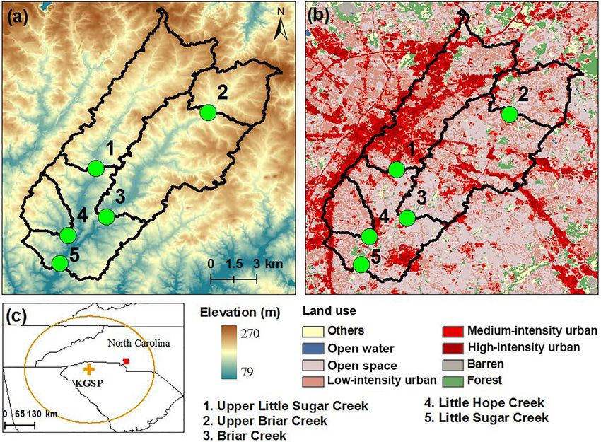
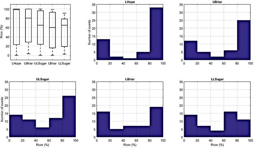
Figure 3. Box plots showing 10, 25, 50, 75 and 90 % quantiles (a) and empirical histograms (b) of fractional basin coverage by maximum
rainfall intensities > 25 mm h−1 , representative of the storm core, for the five basins in the Little Sugar Creek catchment.
Table 2. Overlap in top flood producing storms for the five basins with urbanization effects changing the upper tail of the peak
in Little Sugar Creek catchment, absolute numbers of events. flow distribution, as was suggested by Zhou et al. (2017),
resulting in a different representation of storm events in the
Basin LLSugar LBriar ULSugar UBriar LHope highest quantile peak flows.
name We analyzed relationships between fractional coverage
LLSugar 52 36 36 32 28 and rainfall intensity to see whether changes in basin-average
LBriar 54 30 32 21 rainfall are strongly tied to change in fractional coverage by
ULSugar 69 30 34 the storm core, associated with the storm core moving into
UBriar 50 20 or out of the basin. Spearman rank correlation between first-
LHope 54 order differences in rainfall intensity and rainfall coverage
with time (1R/1t versus 1Rcov /1t) were significant for
all basins, with correlation values varying between 0.38 and
0.69. This confirms that for the selected set of largest flow
similar for Upper compared to Lower LSugar Creek as they events in these basins, change in fractional coverage by the
are for LHope and UBriar or other sets of non-overlapping storm core is an important driver for change in basin-average
basins. Even if flood events in different catchments are gen- rainfall intensity.
erated by the same rainfall events, the characteristics of the
rainfall as it affects the catchments is very different. 3.3 Rainfall position and movement relative to
Figure 4 shows scatter plots of fractional coverage versus flow-path network and effects on hydrological
peak flow. The plots show that there is a tendency for peak response
flows to increase with fractional coverage and that the top
peak flow values are generally associated with 100 % basin An important aim of this study was to investigate how po-
coverage by the storm core. This confirms results found by sition and movement of rainfall in relation to the flow-path
Smith et al. (2002), who concluded that the relation between network, influences hydrological response. Figure 5 shows
storm scale and basin was an important driver for flood re- time-series of basin-average rainfall, fractional coverage by
sponse, and Syed et al. (2003), who found that areal coverage storm core (> 25 mm h−1 ) and normalized RWD and RWD
of the storm core was better correlated with runoff than area dispersion for two selected events in Lower LSugar basin.
coverage of the entire storm. Our results show that for the The two events (Fig. 5a and b) represent events from the top
urbanized basins in Little Sugar Creek, some of the highest 10 highest peak flows in this basin. The third row in the fig-
peak flows (top 10 events in flood catalog) occur for frac- ure illustrates development of normalized RWD as a function
tional coverage well below 100 %. This could be associated of time, the dashed line shows the flow distance for uniform
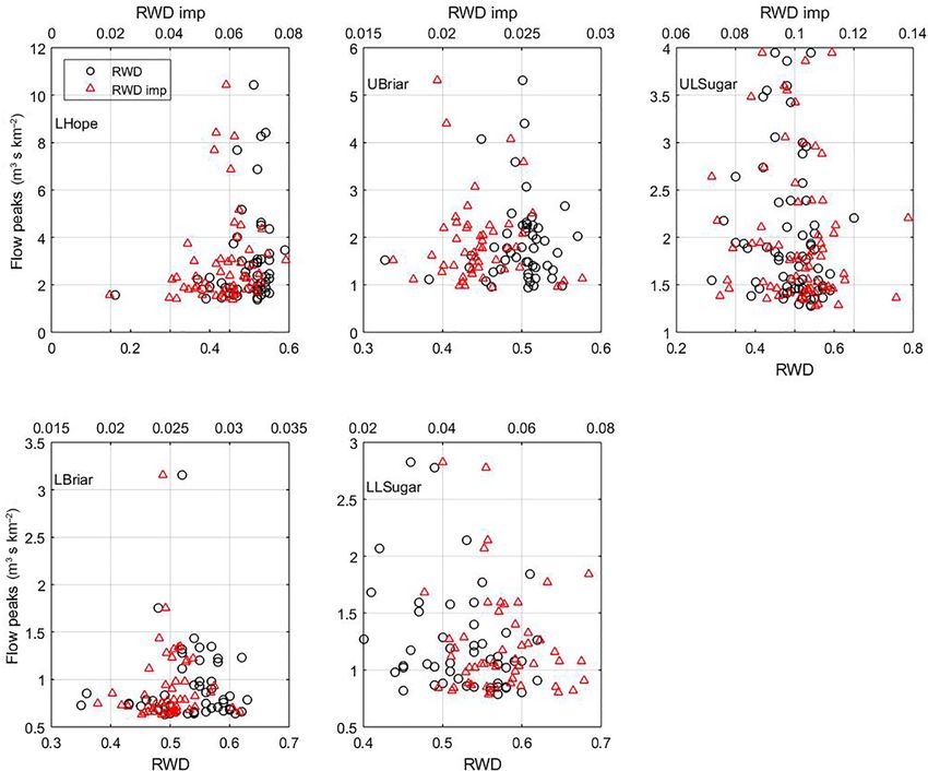
Hydrol. Earth Syst. Sci., 22, 417–436, 2018 www.hydrol-earth-syst-sci.net/22/417/2018/M. ten Veldhuis et al.: The role of storm scale, position and movement in controlling urban flood response 427 Figure 4. Scatter plots of basin fractional coverage by rainfall intensities > 25 mm h−1 versus peak flow, per event, for the five basins in Little Sugar Creek catchment and associated values for Spearman rank correlation coefficients. rainfall, 0.53. The figure shows that normalized RWD values 0.24 of the maximum flow distance (storm centered over the vary in a relatively small range around the mean: mean values outlet corresponds to flow distance value of zero). are 0.41 and 0.40, for a 3 h time window centered on the rain- fall peak. Associated coefficient of variation values are 0.30 and 0.23. This indicates that, on average, rainfall was concen- 3.3.1 Relationship between storm position relative to trated slightly closer to the basin outlet compared to uniform flow-path network and hydrological response rainfall. Normalized RWD dispersion shows whether rainfall is distributed uniformly, unimodally or multimodally with re- Figure 6 shows box plots of normalized RWD values for spect to the flow-path network (see also Eq. 12). Mean nor- event-total accumulated rainfall depth (Fig. 6a) and for the malized RWD dispersion values are 0.83 and 0.93, for a 3 h mean and gradient of 2 h temporally varied RWD (Fig. 6b window centered on the rainfall peak. Maximum normalized and c) for the five basins. Results show that differences in RWD dispersion is 1.04 for the first and 1.39 for the sec- normalized RWD between events tend to be small: 25–75 % ond event. This indicates that on average rainfall was mildly ranges smaller than 0.1 for many of the basins. Differences concentrated in space compared to uniform rainfall, the first increase with a combination of basin size and shape: the event being more unimodal and concentrated in space dur- largest 25–75 and 10–90 % ranges occur for Upper LSugar, ing the peak of the storm and the second event breaking into the most elongated basin (see compactness values Table 1). a multimodal structure in between the two rainfall peaks. This effect is emphasized for normalized RWD dispersion, Storm movement relative to the flow-path network can be where median values are lower and percentile ranges are derived from the time series of normalized RWD, by analyz- much higher for the larger and elongated basins than for the ing gradients in RWD over time. As Fig. 5 shows, normal- two smallest basins (Fig. 6c). These results show that spatial ized RWD was more or less constant during the period of rainfall variability is strongly smoothed by the flow-path net- the most intense rainfall for the first event (cf. period with work and that distribution of rainfall-weighted flow distances rainfall intensities > 25 mm h−1 ), indicating that storm posi- tends to be near uniform for the smallest basins. This sug- tion relative to the flow-path network changed little during gests that the position of the storm relative to the flow-path the event. For the second event, RWD decreased from 0.64 network is likely to affect hydrological response, mainly in to 0.24, the main decrease happening at the same time rain- the larger basins. Relatively more spatially unimodal events fall intensities decreased. This implies that the storm moved occur in the larger and more elongated basins (Fig. 6c), yet into the basin at the upstream end of the flow-path network this does not result in large differences in position along the and moved towards the outlet at the end of the event, to about flow-path network, as indicated by normalized RWD. www.hydrol-earth-syst-sci.net/22/417/2018/ Hydrol. Earth Syst. Sci., 22, 417–436, 2018
428           M. ten Veldhuis et al.: The role of storm scale, position and movement in controlling urban flood response

Figure 5. Time series of basin-average rainfall, flow, portion of basin covered by high-intensity rainfall (> 25 mm h−1 ), normalized
rainfall-weighted flow distance (RWD) and RWD dispersion in Lower LSugar, for two events that occurred on 16 August 2009 (a) and
12 July 2010 (b).

   Figure 7a shows a scatter plot of RWD computed for total          sity; significant correlations were found for mean RWD and
accumulated rainfall depth per storm event versus lag time.          peak flow (LHope, ULSugar, LLSugar), for mean RWD and
For the smaller basins, no clear signal can be observed, yet         lag time (LBriar), and for gradient in RWD with lag time
for the larger basins (Lower Briar and Lower LSugar), lag            (UBriar, LLSugar). Figure 7b shows a scatter plot of maxi-
time was significantly and positively correlated with storm-         mum RWD versus peak flow; the plot shows there is no clear
total RWD. This indicates that in these basins, storm events         relationship between RWDmax and flow peak in LHope,
concentrating in the upstream parts of the flow-path net-            UBriar and LBriar, either because the scale of these basins
work are associated with longer lag times. No significant            is too small compared to the scale of most storms (LHope)
correlations with peak flow were found, as shown in Ta-              or because spatial rainfall variability is strongly smoothed
ble 3, which summarizes Spearman rank correlation values             by the basin (UBriar, LBriar). In ULSugar and LLSugar, the
between storm-total RWD (RWDtot ) and hydrological re-               highest peak flows occur for storms that concentrate over
sponse characteristics, peak flow and lag time.                      the central and downstream parts of the basin, resulting in a
                                                                     negative correlation. A possible explanation for the negative
3.3.2   Relationship between storm movement relative to              correlation between RWD and peak flow for the Upper and
        flow-path network and hydrological response                  Lower LSugar basins is the spatial distribution of impervious
                                                                     areas associated with the urban core of Charlotte. This will
In this section we investigate how the combination of storm          be analyzed in more detail in Sect. 3.4. No significant corre-
position and movement in time influence hydrological re-             lations between RWD and peak flow were found for Upper
sponse. We analyzed correlations with peak flow and lag time         and Lower Briar, which suggests that spatial rainfall distribu-
for minimum, mean, maximum and gradient in normalized                tion does not influence peak flows, possibly due to a strong
RWD over a range of time windows. Table 3 summarizes                 smoothing effect of the flow-path network in these basins.
correlation values for peak flow and lag time, in relation to        Figure 7c shows that large peak flows tend to occur for gradi-
rainfall depth, rainfall intensity and RWD. The highest cor-         ents near zero, i.e. slow-moving, near-stationary storms (rel-
relations were found for rainfall depth and maximum inten-           ative to the flow-path network) or moving storms of larger

Hydrol. Earth Syst. Sci., 22, 417–436, 2018                                         www.hydrol-earth-syst-sci.net/22/417/2018/
M. ten Veldhuis et al.: The role of storm scale, position and movement in controlling urban flood response 429
Figure 6. Box plots of RWD values for storm total rainfall (a); mean RWD for a 2 h window (b) and RWD dispersion for a 2 h window (c),
for all events, for the five basins; scatter plot of mean RWD versus peak flow (d), for Lower LSugar, distinguishing between events with
single and with multiple flow peaks. Red circles in box plots indicate RWD associated with spatially uniform rainfall.
Table 3. Summary of correlations between both peak flow (Qpeak ) and lag time (Tlag ) and total basin-average rainfall (Rtot ), peak rainfall
intensity (Rmax ), normalized RWD associated with storm event total accumulated rainfall (RWDtot ), mean normalized RWD for a 2 h time
window (RWDm ) and gradient in RWD for a 2 h time window (RWDgrad).
Basin Peak flow Lag time
Name vs. Rtot vs. Rmax vs. RWDtot vs. RWDm vs. RWDmax vs. Rtot RWDtot vs. RWDm vs. RWDgrad
LHope 0.30∗ 0.40∗ 0.07 0.31∗ 0.09 0.39∗ 0.20 0.18 −0.08
UBriar 0.32∗ 0.33∗ 0.14 −0.03 −0.03 0.31∗ 0.12 −0.15 −0.37∗
ULSugar 0.49∗ 0.43∗ −0.18 −0.27∗ −0.32∗ 0.29∗ 0.05 −0.08 −0.20
LBriar 0.53∗ 0.38∗ 0.08 0.06 −0.05 0.56∗ 0.41∗ 0.25∗ −0.09
LLSugar 0.48∗ 0.32∗ −0.16 −0.29∗ −0.23 0.43∗ 0.32∗ 0.05 −0.49∗
∗ Indicates significant correlations at the 5 % level.
size than the basin area (especially for smaller basins like by splitting the storm catalog into events with maximum rain-
LHope). fall coverage > 25 mm h−1 above and below 50 %. Correla-
We separately investigated correlations between rainfall- tion values for the two subsets improved for some cases, but
weighted flow distance and hydrological response for a sub- improvements were not consistent across different basins. Fi-
set of clear, single-peak events, to exclude more complex cor- nally, we investigated correlations for a subset of the storm
relation patterns associated with multi-peak events. Single- event catalog, with a strong relation between storm move-
peak events tend to show slightly higher correlations com- ment and rainfall-weighted flow distance, as indicated by
pared to multi-peak events, between rainfall properties or a strong correlation between the two, implying that change
rainfall-weighted flow distances and peak flow or lag time in rainfall intensity is closely associated with rainfall mov-
(Fig. 6d). We also investigated whether correlations were dif- ing across the basin. The number of events with significant
ferent for small-scale storms compared to large-scale storms, 1Rb /1t versus 1DRw /1t correlation varied from 12 for
www.hydrol-earth-syst-sci.net/22/417/2018/ Hydrol. Earth Syst. Sci., 22, 417–436, 2018You can also read